Computer Modeling in Engineering & Sciences

DOI: 10.32604/cmes.2021.016603

ARTICLE

Data-Driven Determinant-Based Greedy Under/Oversampling Vector Sensor Placement

Yuji Saito*, Keigo Yamada, Naoki Kanda, Kumi Nakai, Takayuki Nagata, Taku Nonomura and Keisuke Asai

Tohoku University, Sendai, Miyagi, 980-8579, Japan
*Corresponding Author: Yuji Saito. Email: yuji.saito@tohoku.ac.jp
Received: 11 March 2021; Accepted: 23 June 2021

1  Introduction

Optimal sensor placement is an important challenge in the design, prediction, estimation, and control of high-dimensional systems. High-dimensional states can often leverage a latent low-dimensional representation, and this inherent compressibility enables sparse sensing. For example, in the applications of aerospace engineering, such as launch vehicles and satellites, optimal sensor placement is an important subject in performance prediction, control of the system, fault diagnostics and prognostics, etc. This is because there are limitations of installation, cost, and downlink capacity for transferring measurement data. Reduced-order modeling has been gathering a lot of attention in various fields. A proper orthogonal decomposition (POD) [1,2] is one of the effective methods for decomposing high-dimensional data into several significant modes. Here, POD is a data-driven modal decomposition method that gives the most significant and relevant structure in the data and exactly corresponds to principal component analysis and Karhunen-Loève (KL) decomposition, where the decomposed modes are orthogonal to each other. The POD analysis for a discrete data matrix can be carried out by applying singular value decomposition, as is often the case in the engineering fields. Although there are several advanced data-driven methods, dynamic mode decomposition [3,4], empirical mode decomposition, and others which include efforts by the authors [5,6], this research is only based on the POD which is the most basic data-driven method for reduced-order modeling. If the data can be effectively expressed by a limited number of POD modes, limited sensors placed at appropriate positions will give the information for full state reconstruction. Such effective observation might be one of the keys for flow control and flow prediction. Therefore, the study of optimal sensor placement is important in this field. Such sparse point sensors should be selected considering the POD modes. Although compressed sensing can recover a wider class of signals, the benefits of exploiting known patterns in data with optimized sensing are utilized. Drastic reductions in the required number of sensors and improved reconstruction can be expected in this case. This idea has been adopted by Manohar et al. [7], and the sparse-sensor-placement algorithm has been developed and discussed. The idea is expressed by the following equation:

y=HUz=Cz. (1)

Here, y∈Rp, z∈Rr, H∈Rp×n and U∈Rn×r are the observation vector, the POD mode amplitude, the sparse sensor location matrix, and the spatial POD modes, respectively. In addition, p, n, and r are the number of sensors, the degrees of freedom of the spatial POD modes, and the number of POD modes, respectively. The problem associated with the above equation is considered to be a sensor selection problem when U and strength z are assumed to be a sensor-candidate matrix and the latent state variables, respectively. Joshi et al. defined the objective function for the sensor selection problem, which corresponds to the minimization of the volume of the confidence ellipsoid. They proposed a convex approximation method for this objective function [8]. Recently, Nonomura et al. extended this convex approximation method to a randomized subspace Newton convex approximation method for sparse sensor selection [9], while Nagata et al. proposed an algorithm for another sensor selection method by convex/nonconvex optimizations [10].

Although Joshi et al. proposed a convex approximation method for this objective function [8] as discussed above, the proposed convex approximation methods suffer from a long computational time. Manohar et al. [7] proposed a QR method that provides an approximate greedy solution for the optimization, which is known to be a submatrix volume maximization, and improved the computational time required for the sensor selection problem, relative to the convex approximation method, by using the QR method. The QR method is based on the QR-discrete-empirical-interpolation method (QDEIM) [11,12]. The QR method works well for the sensor selection problem when the number of sensors is less than that of state variables (undersampling). However, the QR method does not seem to connect straightforwardly with the problem y=Cz when a number of sensors is greater than that of state variables (oversampling). Peherstorfer et al. proposed an oversampling-point selection method in the framework of a DEIM-based reduced-order model; the method is based on lower bounds of the smallest eigenvalues of certain structured matrix updates in the case of the number of sensors being greater than that of state variables [13]. They showed that their proposal is almost the best choice among the existing oversampling-point selection methods [7,11,14–16] reported in DEIM studies. Clark et al. extended the idea of the QR method and developed an optimization method for placing sensors under a cost constraint [17–19]. Manohar et al. [20] developed a sensor optimization method using balanced truncation for linear systems. Saito et al. [21] redefined the under/oversampling sensor optimization problems based on the QR method for the scalar-sensor measurement proposed by Manohar et al. [7]. Their method will be called “DG” (D-optimality-based greedy method) in the present study. The objective function of the DG method is based on the D-optimal design of experiments. The DG method is mathematically proved to be the same as the QR method in the undersampled case. In addition, Saito et al. [21] showed that the DG method for the undersampled case is equivalent to the conventional regularized greedy method [22] in the limit where a priori information approaches zero. Nakai et al. investigated the effect of the objective functions on the performance of the sensor selection using the greedy methods [23], that are similarly constructed to that for D-optimality by Saito et al. The objective functions based on D-, A-, and E-optimality, that maximize the determinant, minimize the trace of inverse, and maximize the minimum eigenvalue of the Fisher information matrix, respectively, are adopted to the greedy methods. Yamada et al. proposed the noise-robust greedy method [24]. Their method includes the data-driven noise covariance matrix and Bayesian priors in the objective function and can select the optimal sensor location while considering the correlated noise. Their method will be called “BDG” (Bayesian D-optimality-based greedy method) in the present study. Thus far, the sensor selection problem has been solved by the convex approximation and greedy methods, where the greedy method was shown to be much faster than the convex approximation method [7]. Those ideas are recently applied to several advanced fluid experiments [25–27].

The previous studies introduced so far consider the scalar-sensor measurement that the selected sensors obtain a single component of data at the sensor location. There are several applications of vector-sensor measurement, such as two components of velocity, or simultaneous velocity, pressure, and temperature measurements used in weather forecasting. For example, the real-time particle-image-velocimetry (PIV) measurement of the flowfield is required for the feedback control of a high-speed flowfield in laboratory experiments. The velocity field is calculated from the cross-correlation coefficient for each interrogation window of the particle images in the PIV measurement, but the number of windows that can be processed in a short time is limited because of the high computational costs of the calculation of cross-correlation coefficients. We have been developing a sparse processing particle-image-velocimetry (SPPIV)-measurement system [27]. The key point of this SPPIV-measurement system is the reduction of the amount of processing data and the estimation of the velocity field by a limited number of sparsely located windows, which allows the real-time PIV measurement. The development of an appropriate vector-measurement-sensor selection method is required for the highly accurate SPPIV.

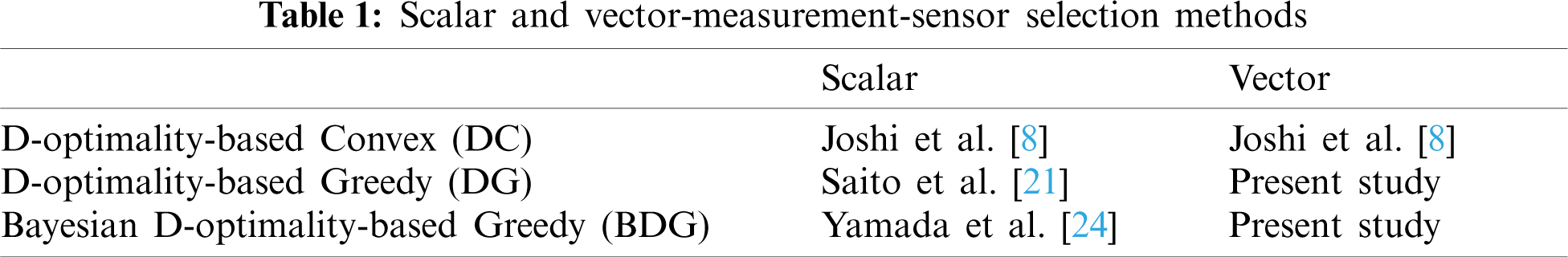
Here, the difference between scalar and vector-sensor measurements is the number of components of data: scalar and vector-sensor measurements obtain a single and multiple components of data at the sensor location, respectively. The extension of the vector-measurement-sensor selection of the convex approximation method has already been addressed in Section C, Chapter V of the original paper [8]. However, the convex approximation method suffers from a long computational time as well as the scalar-measurement-sensor selection problem. Saito et al. straightforwardly extended the greedy algorithm based on the QR method [7] to vector-sensor problems such as fluid dynamic measurement applications [28], but its applications are only limited to undersampled sensors. Therefore, it is necessary to consider the oversampled case and improve the reconstruction accuracy for the high-dimensional data such as fluid dynamic measurement data. In the present study, the more general greedy algorithms based on the D-optimality-based greedy (DG) and Bayesian D-optimality-based greedy (BDG) methods, that were designed for both under and oversampled sensors, are extended to the vector-measurement-sensor selection problem. The effectiveness of these algorithms on the randomly generated systems and practical datasets related to the flowfield around an airfoil and the global climate is demonstrated by comparing the results to those using previously proposed algorithms.

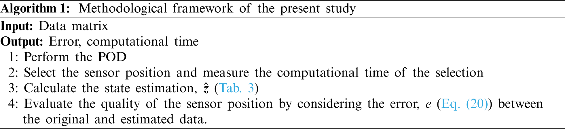
Fig. 1 and Algorithm 1 show the outline of the present study. The data matrix has two or more components as input. For example, in the case of the two-component velocity fields in Fig. 1, the data matrix X=[X1TX2T]T is produced from the lateral velocity data matrix (X1) and the vertical velocity data matrix (X2). After that, a POD analysis is applied to the data matrix X, and a reduced-order model is predefined by the first r low-order POD modes. In addition, the vector-measurement-sensor selection is performed using the POD mode matrix as the sensor-candidate matrix U instead of the scalar that has been studied in previous studies. Although the vector-measurement-sensor selection based on the DC method was proposed by the previous study [8], it suffers from a long computational time. Therefore, the vector-measurement-sensor selections based on the DG and BDG methods are newly developed in the present study. As a result, the calculation time required for vector-measurement-sensor selection is shown to be significantly reduced. Finally, the reconstruction of the multi-components vector fields, such as velocity fields, using the vector-sensor measurement and reduced-order model are demonstrated and evaluated. Tab. 1 summarizes the application range in the present study.

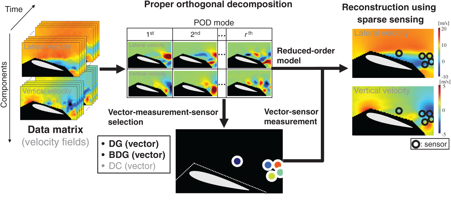
Figure 1: Concept of the present study

The main novelties and contributions of this paper are as follows:

•   The present study extends the DG and BDG methods proposed for scalar-sensor measurements to vector-sensor measurements in the undersampled and oversampled cases.

•   The extensions of the vector-sensor measurement of the DG and BDG methods for the undersampled and oversampled cases have significant novelties for the sparse-sensor measurement in terms of reconstruction error and computational time.

•   The present study compares the performance of the DG and BDG methods with the random selection and DC methods under the conditions: p = 1 −20 at r = 10 (undersampled and oversampled cases) although the previous study [28] considered the vector-sensor selection problem undersampled the undersampled cases.

•   The present study is applied to randomly generated systems and practical datasets of flowfields around the airfoil and global climates. These results illustrate that the proposed DG and BDG methods extended to the vector-measurement-sensor-selection problem are superior to the random selection and DC methods in terms of the accuracy of the sensor selection and computational cost in the present study.

2  Formulation and Algorithms for Sensor Selection Problem

2.1 Scalar-Measurement-Sensor-Selection Problem

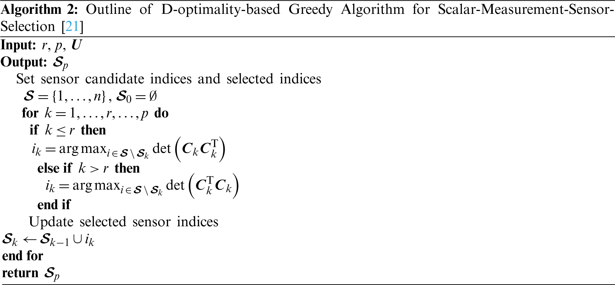
2.1.1 D-Optimality-Based Greedy Algorithm for Scalar-Measurement-Sensor-Selection [21]

A D-optimal design corresponds to maximize the determinant of the Fisher information matrix. Therefore, maximization of the determinant of CCT and CTC for undersampled and oversampled cases are equivalent to minimizing the determinant of the error covariance matrix, resulting in minimizing the volume of the confidence ellipsoid of the regression estimates of the linear model parameters [21,23]. Basically, the exact solution of the scalar-measurement-sensor-selection problem can be obtained by searching all the combinations of p sensors out of n sensor candidates, which takes enormous computational complexity O((n!/(n−p)!/p!))≈O(np). Instead, greedy methods for obtaining the suboptimized solution by adding a sensor step by step have been devised. For the D-optimal criterion, the objective function for the greedy method is demonstrated in the previous study [21]. The subject is summarized in Algorithm 2.

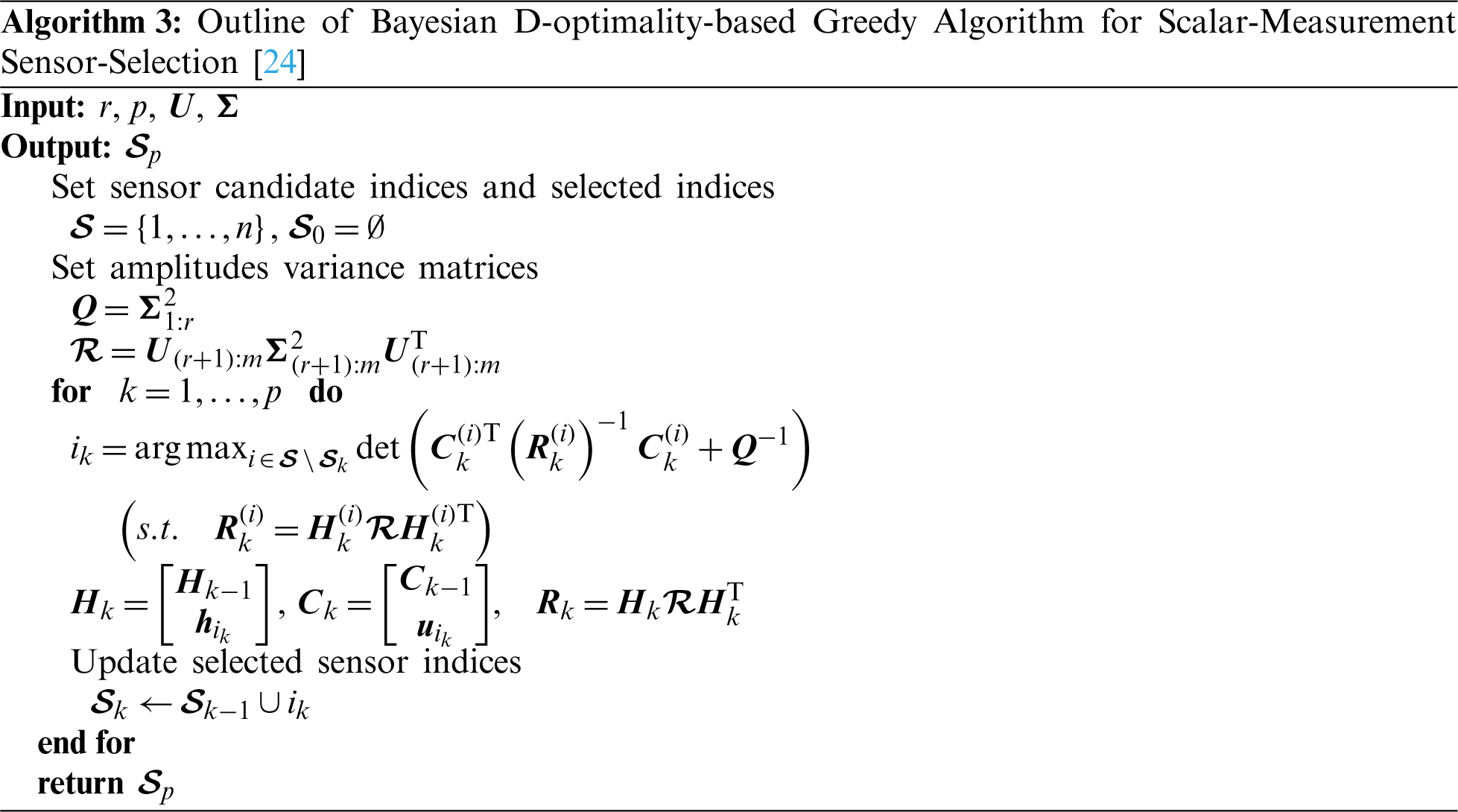
2.1.2 Bayesian D-Optimality-Based Greedy Algorithm for Scalar-Measurement-Sensor-Selection [24]

Improved D-optimality-based greedy algorithm was presented in the previous study [24], and two more priors are exploited for a more robust sensor selection than the D-optimality-based greedy algorithm: one is expected variance of the POD mode amplitudes, and the other is spatial covariance of the components that are truncated in the reduced order-modeling. The former one can be estimated from Σ as:

E(zzT)≡Q≈1mΣ1:rV1:rTV1:rΣ1:r∝Σ1:r2, (2)

where E(θ) is the expectation value of a variable θ. Then, the full-state observation x and the covariance matrix R of the noise become:

x=U1:rz+w,E(wwT)≡R, (3)

where w is a observation noise vector and x is one snapshot (one column vector) of X. The sparse observation and its noise covariance are:

y=HU1:rz+Hw,E(HwwTHT)=HE(wwT)HT≡HRHT≡R, (4)

where R∈Rp×p represents a covariance matrix of the noise that p sensors capture. Here, the full-state noise covariance is assumed to be estimated from the truncated high-order modes when producing a reduced-order model:

R=E(wwT)=E((x−U1:rz)(x−U1:rz)T)≈(UΣVT−U1:rΣrVrT)(UΣVT−U1:rΣrVrT)T=(U(r+1):mΣ(r+1):mV(r+1):mT)(U(r+1):mΣ(r+1):mV(r+1):mT)T=U(r+1):mΣ(r+1):m2U(r+1):mT, (5)

and

R=HRHT≈H(U(r+1):mΣ(r+1):m2U(r+1):mT)HT. (6)

Then, the Bayesian estimation is derived with those prior information. Here, an a priori probability density function (PDF) of the POD mode amplitudes becomes P(z)∝exp⁡(−zTQ−1z) and the conditional PDF of y under given z is as follows P(y∣z)∝exp⁡(−(y−Cz)TR−1(y−Cz)). These relations lead to the a posteriori PDF:

P(z∣y)∝P(y∣z)P(z)∝exp⁡(−(y−Cz)TR−1(y−Cz))exp⁡(−zTQ−1z)=exp⁡(−(y−Cz)TR−1(y−Cz)−zTQ−1z). (7)

Here, the maximum a posteriori estimation on p(z∣y) is z^=(CTR−1C+Q−1)−1CTR−1y. Owing to the normalization term Q, the inverse operation is regular for any conditions of p unlike the least squares estimation. In this estimation, the objective function of the BDG method is modified as the maximization of the determinant of (CTR−1C+Q−1). The BDG method selects sensor set Sp that are robust against covariance noise represented by R. The algorithm of the BDG method is summarized in Algorithm 3.

2.2 Vector-Measurement-Sensor-Selection Problem

A vector-measurement-sensor-selection problem in the undersampled and oversampled cases is considered by extending the previously explained DG and BDG methods. Again, the number of components of data is different for scalar and vector-sensor measurements: scalar and vector-sensor measurements obtain a single and multiple components of data at the sensor location, respectively. In the vector-sensor measurement, the following equation is considered:

y=[I⊗hi1I⊗hi2⋮I⊗hik][U1U2⋮Us]z=[hi10⋯00hi1⋯000⋱0000hi11−4hi20⋯00hi2⋯000⋱0000hi21−4⋮⋮⋮⋮1−4hik0⋯00hik⋯000⋱0000hik][U1U2⋮Us]z=[Hs1Hs2⋮Hsk][U1U2⋮Us]z=Πk[U1U2⋮Us]z=[W1W2⋮Wk]z=Dz (8)

Here, Us∈Rns×r is the sth vector component of a sensor-candidate matrix, Hsk∈Rs×n and Πk∈Rsk×n are the sensor location matrix for each vector component and the vector-measurement-sensor location matrix for first-to-kth sensors, where s is the number of components of the measurement vector and the condition s < r is assumed in the present study. Again, p and r are the numbers of sensors and latent state variables, respectively, and n is the number of spacial dimensions including the different vector components. Let Wi∈Rs×r denotes the vector sensor-candidate matrix as follows:

Wi=[ui,1Tui,2T…ui,s−1Tui,sT]T, (9)

where ui,s∈R1×r is the corresponding row vector of the sensor-candidate matrix. Let Dk∈Rs×r denotes the kth vector sensor-candidate matrix as follows:

Dk=[Wi,1TWi,2T…Wi,k−1TWi,kT]T. (10)

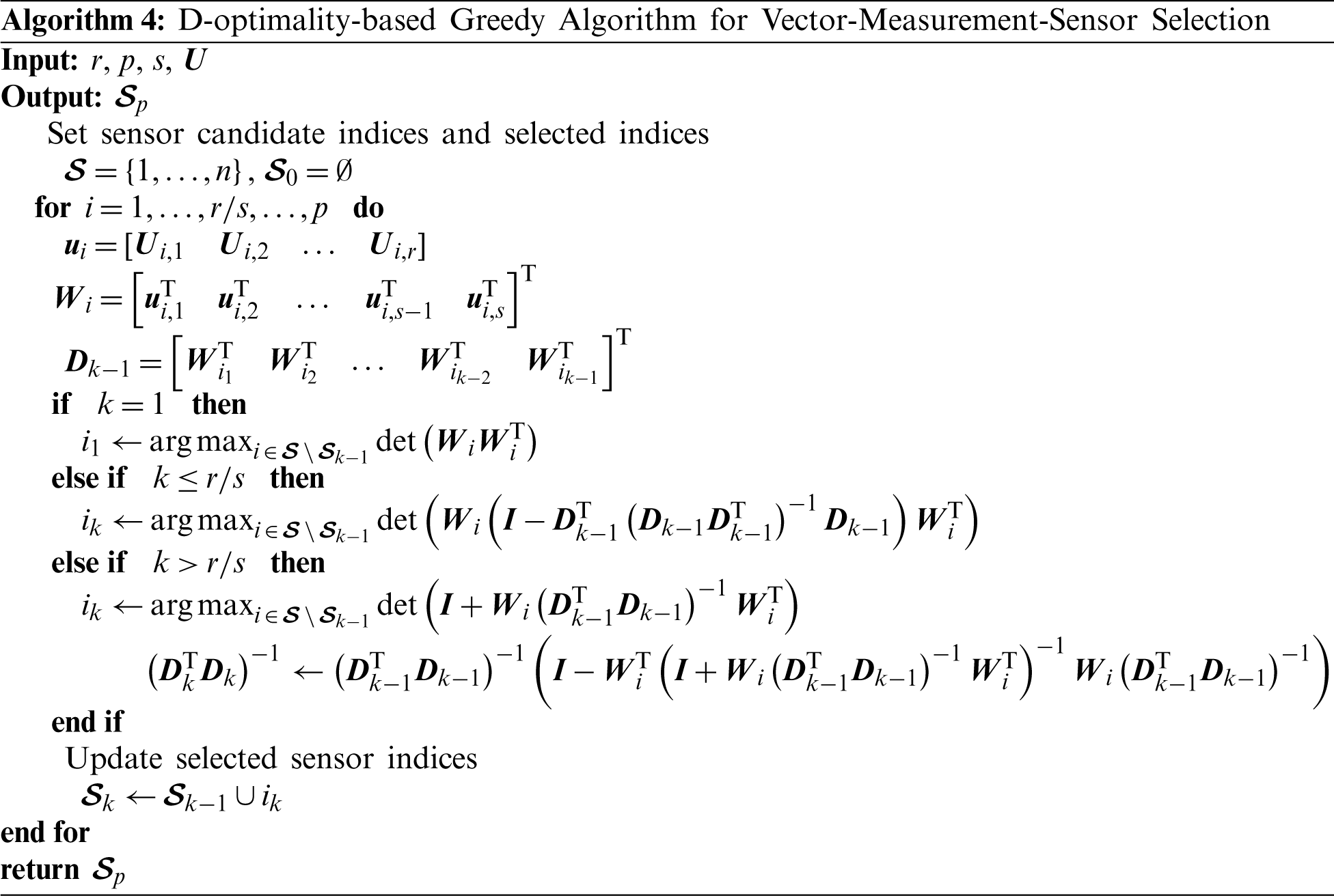
2.2.1 D-Optimality-Based Greedy Algorithm for Vector-Measurement-Sensor Selection

The algorithm of the DG method for vector-measurement sensors in the undersampled and oversampled cases is summarized in Algorithm 4.

The step-by-step maximization of the determinant of DkDkT is conducted using the greedy method in the case of k≤r. This objective is the maximization of the determinant of the matrix appearing in pseudo inverse matrix operations, leading to the minimization of the volume of the confidence ellipsoid. It can be expanded as follows (see, e.g., [29] for detailed derivation):

det(DkDkT)=det([Dk−1Wi][Dk−1TWiT])=det([Dk−1Dk−1TDk−1WiTWiDk−1TWiWiT])=det(Wi(I−Dk−1T(Dk−1Dk−1T)−1Dk−1)WiT)det(Dk−1Dk−1T), (11)

and therefore,

ik=argmaxi∈S∖Skdet(DkDkT)=argmaxi∈S∖Skdet(Wi(I−Dk−1T(Dk−1Dk−1T)−1Dk−1)WiT). (12)

In the undersampled case, the DG method is the same as the vector-measurement sensor selection method [28] which was developed based on the QR method, though the mathematical proof was omitted for brevity. Many previous studies have been conducted with the aim of reduction in the numerical instability and the computational cost when the QR decomposition is applied to the “tall-skinny matrices” [30]. Although there may be a possibility of numerical instability related to the QR decomposition for tall-skinny matrices, the numerical instability of the DG method proposed in the present study has not been observed in our experiences.

The maximization of the determinant of DTD is simply considered in the case of k≥r/s (see, e.g., [29] for detailed derivation):

Therefore,

ik=argmaxi∈S∖Skdet(Dk−1TDk−1+WiTWi)=argmaxi∈S∖Skdet(I+Wi(Dk−1TDk−1)−1WiT). (13)

The complexity when searching all components of the vector becomes O(nr2s4) when inverse (Dk−1TDk−1)−1 is known. The inverse (DkTDk)−1 can be computed recursively using a matrix inversion lemma when a new sensor is found and the step number k is incremented, as follows:

(DkTDk)−1=(Dk−1TDk−1+WiTWi)−1=(Dk−1TDk−1)−1(I−WiT(I+Wi(Dk−1TDk−1)−1WiT)−1Wi(Dk−1TDk−1)−1). (14)

The size of the matrix is s×s, and the computational cost of the proposed method is significantly lower than that of the original objective functions: sp×sp and r×r in the undersampled and oversampled cases. The sensor-candidate matrix is assumed to be a full-column-rank matrix in the DG method. This is because the unobservable subspace in the latent variables does not exist, and any latent variables are assumed to be observed by at least one of the sensor candidates in oversampled cases. It will be difficult to apply the method proposed above, when the number of s is so large that the vector components of the sensor matrix could not be linearly independent. In that case, sensors can be selected by considering the determinant of CTC+ϵI for both undersampled and oversampled sensors in modified Eq. (13), though the sufficiently small number ϵ should be determined by try-and-error processes. Although the use of ϵI, which has been discussed in Refs. [21,22] for the scalar-sensor measurements, is not recommended because it introduces the hyperparameter ϵ, it makes the computation stable in the difficult situations of the vector sensors that are not linearly independent. When the number of s is relatively small and the vector components of the sensor matrix are linearly independent as in the case discussed in the present study, the proposed method works well as described later.

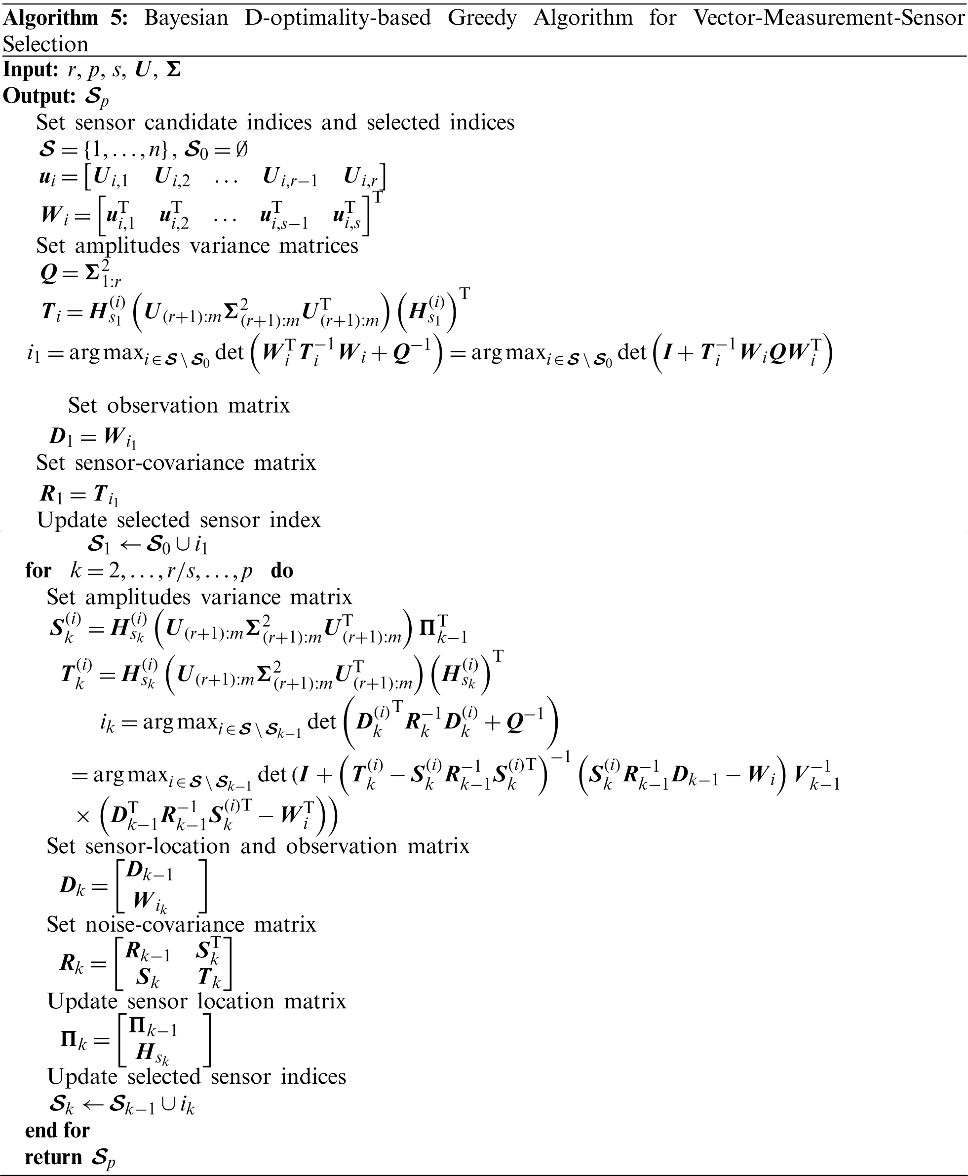
2.2.2 Bayesian D-Optimality-Based Greedy Algorithm for Vector-Measurement-Sensor Selection

A fast implementation is considered as Saito et al. demonstrated in their determinant calculation using rank-one lemma [21]. First, the covariance matrix generated by the ith sensor candidate in the kth sensor selection, Rk(i) is:

Rk(i)=(Rk−1Sk(i)TSk(i)Tk(i)), (15)

where the covariance Sk(i) of noise between the sensor candidate i and the (k−1) selected sensors is

Sk(i)∝E(HskwwTΠk−1T)=HskE(wwT)Πk−1T=HskRΠk−1T≈Hsk(U(r+1):mΣ(r+1):m2U(r+1):mT)Πk−1T, (16)

and similarly, the variance of noise is defined as:

Tk(i)=Hsk(U(r+1):mΣ(r+1):m2U(r+1):mT)HskT. (17)

In addition, Rk−1 is determined in the previous (k−1)th step. Accordingly, (Rk(i))−1 is obtained as follows:

(Rk(i))−1≡(αk(i)βk(i)Tβk(i)δk(i)), (18)

where

The objective function of BDG is now considered based on the expressions above.

Because Vk−1 and its determinant have already been obtained in the previous step, the kth sensor can be selected by the following evaluation:

ik=argmaxi∈S¯∖Skdet(I+(Tk(i)−Sk(i)Rk−1−1Sk(i)T)−1(Sk(i)Rk−1−1Dk−1−Wi)Vk−1−1(Dk−1TRk−1−1Sk(i)T−WiT)). (19)

Once the sensor is selected, Rk−1 and Vk are updated. The algorithm of the BDG method for vector-measurement-sensor selection is described in Algorithm 5. The previous study in the scalar-measurement-sensor-selection problem proposes the implementation reducing the order of the noise covariance from (m−r) to r2 and reduces the computational complexity [24]. This process is called the r2 truncation in the previous study. Although the r2 truncation will reduce the computational complexity in the vector-measurement-sensor-selection problem, the r2 truncation is not addressed in the present study. This is because it additionally needs to conduct the parametric study for the reasonable r2, and the extensions of the vector-measurement-sensor selection of the DG and BDG methods are focused in the present study.

3  Results and Discussion

The numerical experiments are conducted and the proposed methods are validated. The random sensor, PIV, and NOAA-SST/ICEC problems are applied in the present study. The vector sensor-measurement matrix U for each case is predefined by the POD bases. Hereinafter, four different implementations are compared: the random selection, DC, DG, and BDG methods. The random selection and convex approximation methods [8] are evaluated as the references. All numerical experiments are solved under the computational environments listed in Tab. 2.

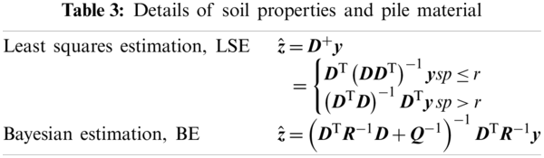
The quality of the sensors is evaluated by considering the error between the original and estimated data. The error e is defined as below:

e=‖X−UZ^‖F‖X‖F. (20)

Here, series of the estimation z~ in or are concatenated as Z^, and ‖∘‖F is taking matrix norm of ∘. The state estimation methods are presented in Tab. 3. For example, the DG (scalar)-LSE method represents the combination method using the scalar-measurement-sensor selection based on the DG method and the least squares estimation method, and the BDG (vector)-BE method represents the combination method using the vector-measurement-sensor selection based on the BDG method and the Bayesian estimation method. In the full observation, the state estimation is calculated as follows: Z^=UUTX. In the PIV and NOAA-SST/ICEC problems, the errors will be discussed in two cases in which the training and validation data are the same as each other and in which the training and validation data are different. In the case of the training and validation data are different, a K-fold cross-validation (K = 5) is conducted, and the performances of algorithms are compared. The m snapshots are partitioned into five segments. Each of the five data segments is used as the validation data with the remaining data used for training and the estimation error is evaluated.

3.1 Random Sensor Problem

The random data matrices, Xrand=UΣVT(Xrand∈R1000×100), were set, where U and V consist of 100 orthogonal vectors that were generated by QR decomposition of normally distributed random matrices, and components of diagonal matrix Σ were diag(Σ)=[1,12,13,...,1100], respectively. Fig. 2 shows the relationship between the errors of the results using the DG (scalar)-LSE (dot black line with opened circle), DG (vector)-LSE (solid black line with closed circle), BDG (scalar)-BE (dot red line with opened circle) and BDG (vector)-BE methods (solid red line with closed circle) in the random sensor problem (n = 1000, m = 100, s = 2, and r = 10). The errors of the results using the DG (vector)-LSE and BDG (vector)-BE methods, which are extended to the vector-sensor measurement in the present study, are smaller than those of the results using the DG (scalar)-LSE and BDG (scalar)-BE methods, respectively in the random sensor problem. Fig. 3 shows the relationship between the errors of the results using the random (vector)-LSE (solid gray line with closed circle), DC (vector)-LSE (solid blue line with closed circle), DG (vector)-LSE (solid black line with closed circle) methods and the number of sensors in the random sensor problem. All the errors are averaged over 1000 trials. Because C which is determined by the sensor selection is not a regular matrix, all the errors estimated by the least squares estimation (LSE) increase in the case of sp≈r. The error of the results using the DG (vector)-LSE, which is extended to the vector-sensor measurement in the present study, is the smallest as shown in Fig. 3. Fig. 4 shows the relationship between the errors of the results using the random (vector)-BE (solid gray line with closed circle), DC (vector)-BE (solid blue line with closed circle), DG (vector)-BE (solid black line with closed circle), BDG (vector)-BE (solid red line with closed circle) methods and the number of sensors in the random sensor problem. All the errors estimated by the Bayesian estimation (BE) are again smaller than those estimated by LSE shown in Fig. 3 and monotonically decrease as the number of sensors increases. Although the difference between the errors of the results using the DC (vector)-BE, DG (vector)-BE and BDG (vector)-BE methods is large in the case of p≤5, the error difference between them disappears in the case of p > 5. The error of the results using the BDG (vector)-BE method, which is extended to the vector-sensor measurement in the present study, is the smallest.

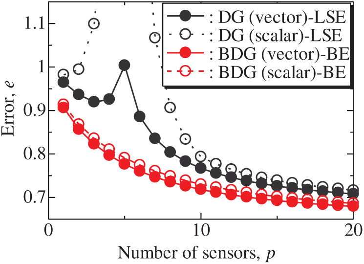
Figure 2: Errors of the results using the DG (scalar)-LSE, DG (vector)-LSE, BDG (scalar)-BE and BDG (vector)-BE methods against the number of sensors in the random sensor problem: n = 1000, m = 100, r = 10, s = 2

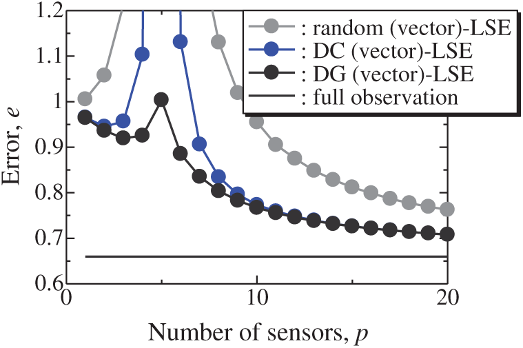
Figure 3: Errors of the results using the random (vector)-LSE, DC (vector)-LSE, and DG (vector)-LSE methods against the number of sensors in the random sensor problem: n = 1000, m = 100, r = 10, s = 2

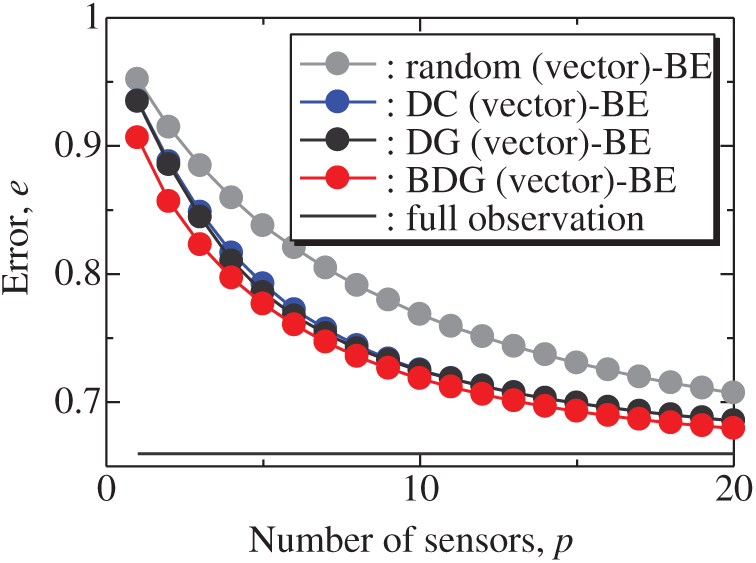
Figure 4: Errors of the results using the random (vector)-BE, DC (vector)-BE, DG (vector)-BE, and BDG (vector)-BE methods against the number of sensors in the random sensor problem: n = 1000, m = 100, r = 10, s = 2

Fig. 5 shows the relationship between the computational time of the results using the random (vector), DC (vector), DG (vector), and BDG (vector) methods and the number of sensors p in the random sensor problem. The random (vector) and DC (vector) methods take a certain amount of time regardless of the number of sensors, and the DC method has a particularly high calculation cost. The computational times of the DG (vector) and BDG (vector) methods increase monotonically as the number of sensors increases since the sensors are determined greedily. In this random problem, the computational time of the DG (vector) method is much shorter than that of the DC (vector) method, and the computational time of the BDG (vector) method is shorter than that of the DC method in the case of p≤13. The BDG (vector) method takes longer time to calculate than the DC (vector) method in the case of p > 13, though the BDG (vector) method has the smallest error in the random sensor problem. Although the r2 truncation proposed in the previous study for the scalar-measurement-sensor-selection problem [24] is not addressed in the random sensor selection problem, the r2 truncation for the BDG (vector) method will reduce the computational time. The DG (vector) method which has the same error as the DC method is computationally fast, and the two methods extended in the present study are generally better methods in the random sensor problem.

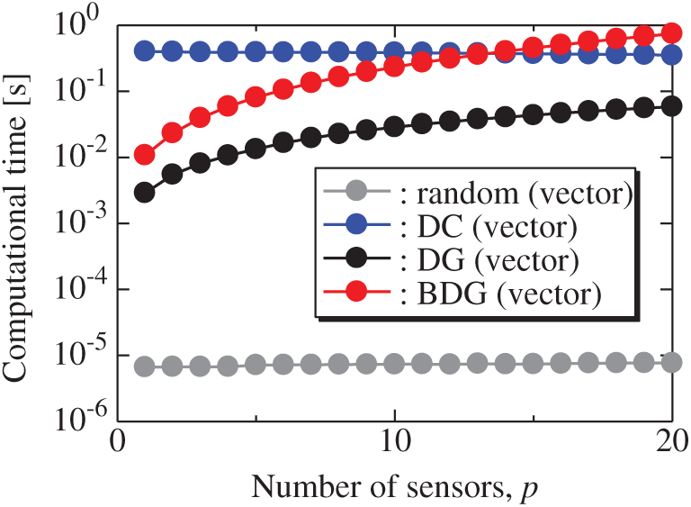
Figure 5: Computational times of the results using the random (vector), DC (vector), DG (vector), and BDG (vector) methods against the number of sensors in the random sensor problem: n = 1000, m = 100, r = 10, s = 2

3.2 PIV

The particle image velocimetry (PIV) for acquiring time-resolved data of velocity fields around an airfoil was conducted previously [31]. The effectiveness of the present method for the PIV data is demonstrated hereafter. Here, the overview of the experimental data is briefly explained. The wind-tunnel test was conducted in the Tohoku-university Basic Aerodynamic Research Wind Tunnel (T-BART) with a closed test section of 300 mm × 300 mm cross-section. The airfoil of the test model had an NACA0015 profile, the chord length and span width of which were 100 and 300 mm, respectively. The freestream velocity U∞ and attack angle of the airfoil α were set to be 10 m/s and 16 degrees, respectively. The chord Reynolds number was 6.4 × 104. Time-resolved PIV measurement was conducted with a double-pulse laser. The sampling rate at which the velocity fields are acquired, the particle image resolution, and the total number of snapshots were 5000 Hz, 1024 × 1024 pixels, and m = 1000, respectively. The tracer particles were 50% aqueous solution of glycerin with estimated diameter of a few micrometers. The particle images were acquired by using the double pulse laser (LDY-300PIV, Litron) and a high-speed camera (SA-X2, Photron) which were synchronized to each other. These PIV data with noise were obtained through real wind-tunnel experiments.

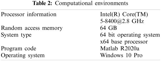
The vector-measurement-sensor selection problem for the reconstruction of the lateral and vertical components of the velocities measured by PIV (Figs. 6 and 7) is solved using the same computational environments listed in Tab. 2 as those used in the random sensor problem. Fig. 8 shows the relationship between the errors of the results using the DG (vector)-LSE, DG (scalar, lateral)-LSE, DG (scalar, vertical)-LSE, BDG (vector)-BE, BDG (scalar, lateral)-BE and BDG (scalar, vertical)-BE methods in the PIV problem (n = 6096, m = 1000, r = 10, and s = 2), where the lateral and vertical represent the lateral and vertical components of the velocity fields. The errors of the results using the DG (vector)-LSE and BDG (vector)-BE methods, which are extended to the vector-sensor measurement in the present study, are smaller than those of the results using the DG (scalar, lateral and vertical)-LSE methods and the BDG (scalar, lateral and vertical)-BE methods, respectively in the PIV problem. Fig. 9 shows the snapshots of the original and reconstructed data by the random (vector)-LSE, DC (vector)-LSE, and DG (vector)-LSE, respectively in the cases of sp = r = 10. The black open circles show the sensor positions selected by each method. The random (vector)-LSE method cannot correctly reconstruct the velocity fields compared to those of the original data. On the other hand, the velocity fields reconstructed by the DC (vector)-LSE and DG (vector)-LSE methods are almost the same as the velocity fields of the original data. Figs. 10 and 11 show the relationships between the errors of the results using the random (vector)-LSE, DC (vector)-LSE, and DG (vector)-LSE methods and the number of sensors for the PIV problem in which the training and validation data are the same as each other and in which the training and validation data are different (K-fold cross-validation, K = 5). The error of the results using the random (vector)-LSE is averaged over 1000 trials. The error bars represent the standard deviations of the five calculations in Fig. 11. All the errors increase in the case of sp≈r because C which is determined by the sensor selection is not a regular matrix, as shown in Figs. 10 and 11 as well as that shown in Fig. 3. The error of the results using the DG (vector)-LSE method is smaller than or the same as the error of the results using the DC (vector)-LSE method and is lower than that of the results using the random (vector)-LSE method.

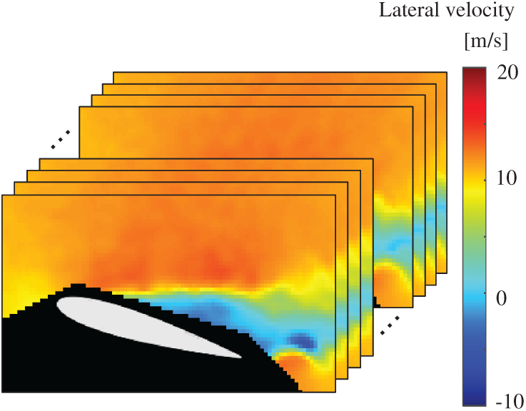
Figure 6: Dataset of PIV: snapshots of the lateral-velocity field

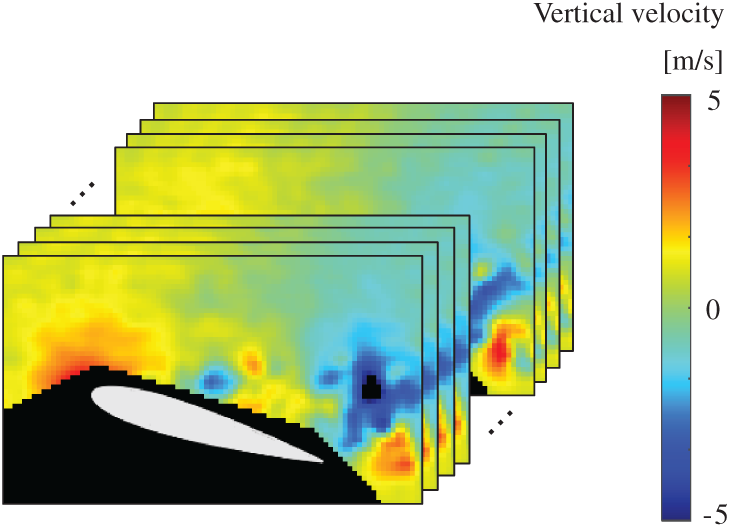
Figure 7: Dataet of PIV: snapshots of the vertical-velocity field

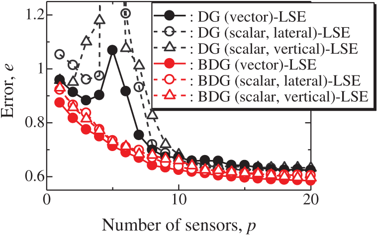
Figure 8: Errors of the results using the DG (vector)-LSE, DG (scalar, lateral)-LSE, DG (scalar, vertical)-LSE, BDG (vector)-BE, BDG (scalar, lateral)-BE and BDG (scalar, vertical)-BE methods against the number of sensors in the PIV problem: n = 6096, m = 1000, r = 10, p = 5 and s = 2

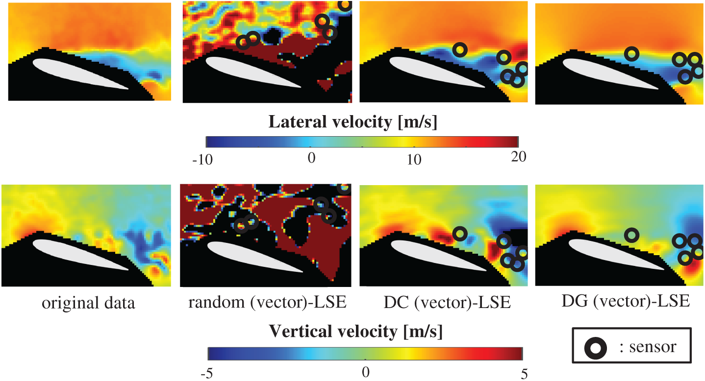
Figure 9: Single snapshots of the original data and reconstructed velocity fields by the random (vector)-LSE, DC (vector)-LSE, and DG (vector)-LSE methods, respectively in the PIV problem: n = 6096, m = 1000, r = 10, p = 5 and s = 2

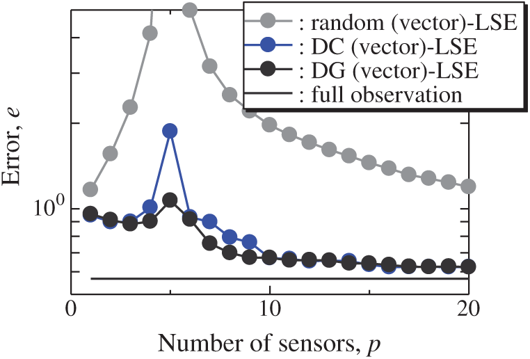
Figure 10: Errors of the results using the random (vector)-LSE, DC (vector)-LSE, DG (vector)-LSE methods against the number of sensors in the PIV problem: n = 6096, m = 1000, r = 10, s = 2

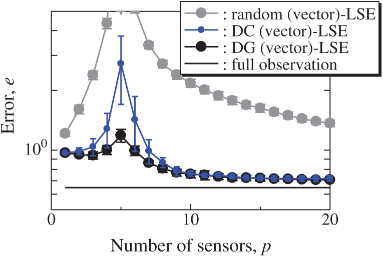
Figure 11: Errors of the K-fold cross-validation results using the random (vector)-LSE, DC (vector)-LSE, DG (vector)-LSE methods against the number of sensors in the PIV problem: n = 6096, m = 1000, r = 10, s = 2, and K = 5

Fig. 12 shows the snapshots of the reconstructed data by the BDG (vector)-BE, random (vector)-BE, DC (vector)-BE and DG (vector)-BE methods, respectively in the cases of sp = r = 10. The velocity fields reconstructed by the BDG (vector)-BE, random (vector)-BE, DC (vector)-BE and DG (vector)-BE methods are almost the same as the velocity fields of the original data as shown in Fig. 9. Figs. 13 and 14 show the relationship between the errors of the results using the random (vector)-BE, DC (vector)-BE, DG (vector)-BE and BDG (vector)-BE methods and the number of sensors for the PIV problem in which the training and validation data are the same as each other and in which the training and validation data are different (K-fold cross-validation, K = 5). All the errors estimated by the BE method are smaller than those estimated by the LSE method in as shown in Figs. 10 and 11, and monotonically decrease as the number of sensors increases as well as the random sensor problem. The error of the BDG (vector)-BE method, which extended to the vector-sensor measurement in the present study is the smallest in this PIV problem. Although Loiseau et al. show the two-dimensional cylinder flow reconstructed by the selected five sensors [32], the sensors are selected by the scalar-sensor measurement based on the QR method [7]. Therefore, their results will be improved by the DG (vector) and BDG (vector) methods extended to the vector-sensor measurement. Fig. 15 shows the relationship between the computational time and the number of sensors p in the PIV problem. As well as the random sensor problem, the random (vector) and DC (vector) methods take a certain amount of time regardless of the number of sensors. The computational times of the DG (vector) and BDG (vector) methods increase monotonically as the number of sensors increases since the sensors are determined greedily. The BDG (vector) method takes longer to calculate than the DC (vector) method in the case of p > 10, however, the BDG (vector) method has the smallest error in the PIV problem as shown in Figs. 13 and 14. The r2 truncation [24] for the BDG (vector) method will reduce the computational time although the r2 truncation is not addressed in the PIV problem. The DG (vector) method which has the same error as the DC (vector) method is faster than the BDG (vector) and DC (vector) methods. Therefore, the BDG (vector) and DG (vector) methods extended in the present study are better methods in the PIV problem obtained through real wind-tunnel tests.

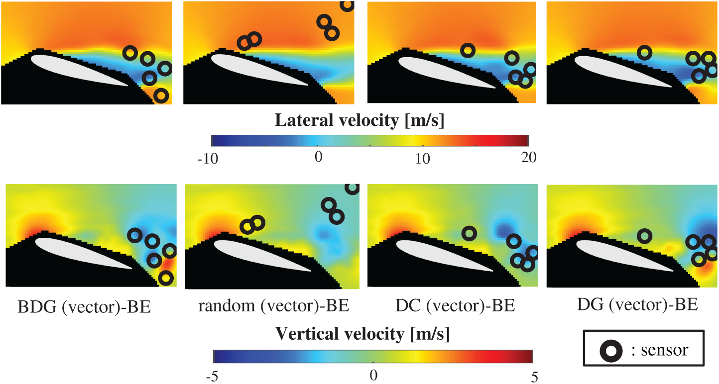
Figure 12: Single snapshots of the reconstructed velocity fields by the BDG (vector)-BE, random (vector)-BE, DC (vector)-BE and DG (vector)-BE methods, respectively in the PIV problem: n = 6096, m = 1000, r = 10, p = 5 and s = 2

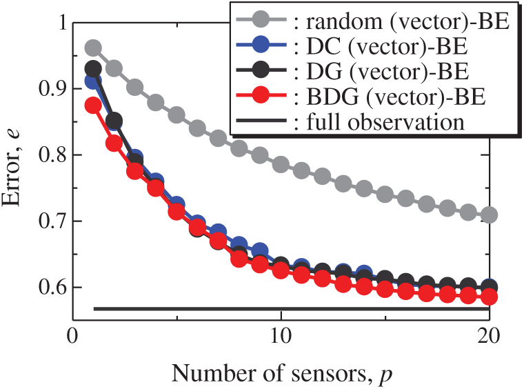
Figure 13: Errors of the results using the random (vector)-BE, DC (vector)-BE, DG (vector)-BE and BDG (vector)-BE methods against the number of sensors in the PIV problem: n = 6096, m = 1000, r = 10 and s = 2

Figure 14: Errors of the K-fold cross-validation results using the random (vector)-BE, DC (vector)-BE, DG (vector)-BE and BDG (vector)-BE methods against the number of sensors in the PIV problem: n = 6096, m = 1000, r = 10, s = 2, and K = 5

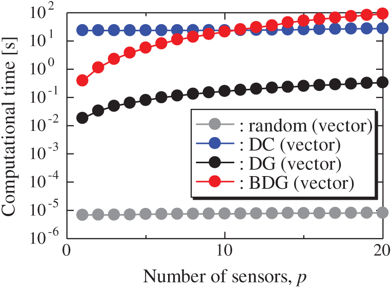
Figure 15: Computational times of the results using the random (vector), DC (vector), DG (vector), and BDG (vector) methods against the number of sensors in the PIV problem: n = 6096, m = 1000, r = 10 and s = 2

3.3 NOAA-SST/ICEC

The data set that we finally adopt is the NOAA OISST V2 mean sea surface dataset (NOAA-SST/ICEC), comprising weekly global sea surface temperature in Fig. 16) and ice concentrations (Fig. 17) in the years between 1990 and 2000 (m = 520) [33]. There are a total of 520 snapshots on a 360 × 180 spatial grid (Figs. 16 and 17). The vector-measurement-sensor-selection problem for NOAA-SST/ICEC is solved using the same computational environments in Tab. 2 as those used in the problems of the random sensor and PIV. In this NOAA-SST/ICEC problem, the locations are beforehand excluded from S for simplicity if their RMSs are 10−1 times smaller than the maximum of those of the dataset, and S¯ denotes a subset of S after this exclusion.

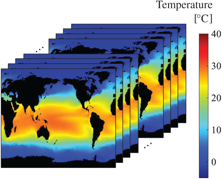
Figure 16: Dataset of NOAA-SST/ICEC: snapshots of the sea-surface-temperature filed

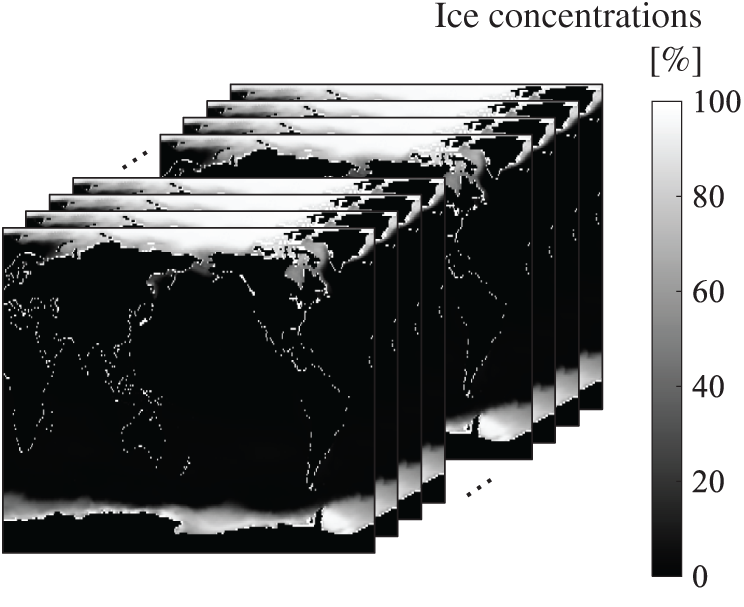
Figure 17: Dataset of NOAA-SST/ICEC: snapshots of the ice-concentrations field

Fig. 18 shows the relationship between the errors of the results using the DG (vector)-LSE, DG (scalar, SST)-LSE, DG (scalar, ICEC)-LSE, BDG (vector)-BE, BDG (scalar, SST)-BE and BDG (scalar, ICEC)-BE methods in the NOAA-SST/ICEC problem (n = 88438, m = 520, s = 2, and r = 10), where SST and ICEC represent the sea surface temperature and ice concentrations, respectively. The errors of the results using the DG (vector)-LSE and BDG (vector)-BE methods, which are extended to the vector-sensor measurement in the present study, are smaller than those of the results using the DG (scalar, SST and ICEC)-LSE methods and the BDG (scalar, SST and ICEC)-BE methods, respectively in the NOAA-SST/ICEC problem. Fig. 19 shows the snapshots of the original and reconstructed data by the random (vector)-LSE, DC (vector)-LSE, and DG (vector)-LSE methods, respectively in the cases of sp = r = 10. The yellow open circles show the sensor positions selected by each method. The random (vector)-LSE and DC (vector)-LSE methods cannot correctly reconstruct the snapshots compared to those of the original data. On the other hand, the snapshots of the reconstructed fields data by the DG (vector)-LSE method are almost the same as those of the original data. Figs. 20 and 21 show the relationships between the errors of the results using the random (vector)-LSE, DC (vector)-LSE, DG (vector)-LSE methods and the number of sensors for the NOAA-SST/ICEC problem in which the training and validation data are the same as each other and in which the training and validation data are different (K-fold cross-validation, K = 5). The error of the results using the random (vector)-LSE is averaged over 1000 trials. The error bars represent the standard deviations of the five calculations in Fig. 21. All the errors increase in the case of sp≈r because C which is determined by the sensor selection is not a regular matrix, as shown in Figs. 20 and 21 as well as that shown in Figs. 3, 10 and 11. The error of the results using the DG (vector)-LSE method is smaller than or the same as the error of the results using the DC (vector)-LSE method and is further lower than that of the results using the random (vector)-LSE method.

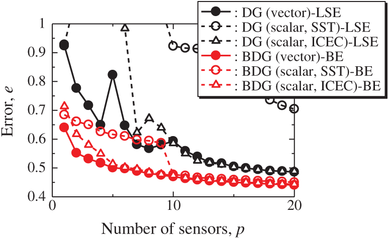
Figure 18: Errors of the results using the DG (vector)-LSE, DG (scalar, SST)-LSE, DG (scalar, ICEC)-LSE, BDG (vector)-BE, BDG (vector)-BE, BDG (scalar, SST)-BE and BDG (scalar, ICEC) methods against the number of sensors in the NOAA-SST/ICEC problem: n = 88438, m = 520, r = 10, p = 5, and s = 2

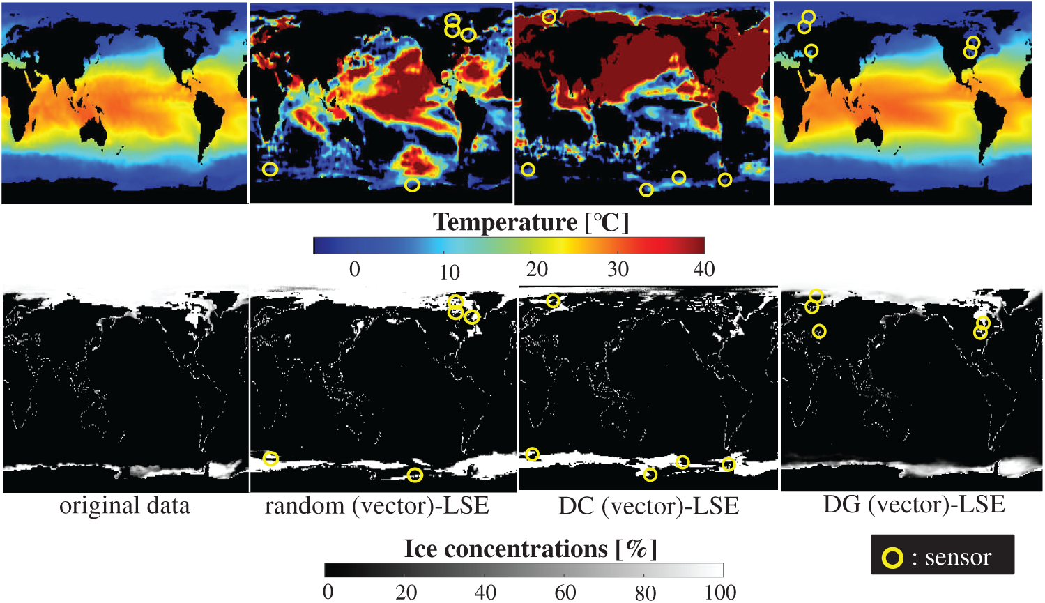
Figure 19: Single snapshots of the original data and reconstructed fields data by the random (vector)-LSE, DC (vector)-LSE, and DG (vector)-LSE methods, respectively in the NOAA-SST/ICEC problem: n = 88438, m = 520, r = 10, p = 5, and s = 2

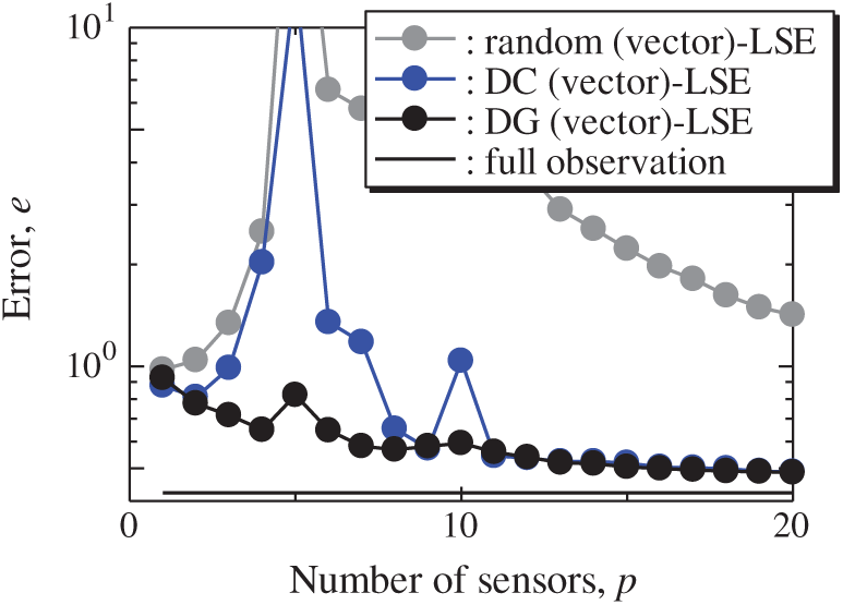
Figure 20: Errors of the results using the random (vector)-LSE, DC (vector)-LSE and DG (vector)-LSE methods against the number of sensors in the NOAA-SST/ICEC problem: n = 88438, m = 520, r = 10, and s = 2

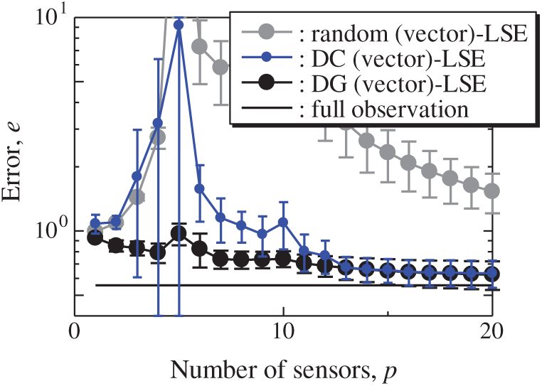
Figure 21: Errors of the K-fold cross-validation results using the random (vector)-LSE, DC (vector)-LSE and DG (vector)-LSE methods against the number of sensors in the NOAA-SST/ICEC problem: n = 88438, m = 520, r = 10, s = 2, and K = 5

Fig. 22 shows the snapshots of the reconstructed data by the BDG (vector)-BE, random (vector)-BE, DC (vector)-BE, and DG (vector)-BE methods, respectively in the cases of sp = r = 10. The random (vector)-LSE and DC (vector)-LSE methods cannot correctly reconstruct the snapshots compared to those of the original data. On the other hand, the snapshots of the reconstructed fields data by the DG (vector)-LSE method are almost the same as those of the original data. The snapshots of the reconstructed data by the BDG (vector)-BE, random (vector)-BE, DC (vector)-BE and DG (vector)-BE methods are almost the same as the snapshot of the original data as shown in Fig. 19. Figs. 23 and 24 show the relationships between the errors of the results using the random (vector)-BE, DC (vector)-BE, DG (vector)-BE methods and the number of sensors for the NOAA-SST/ICEC problem in which the training and validation data are the same as each other and in which the training and validation data are different (K-fold cross-validation, K = 5).

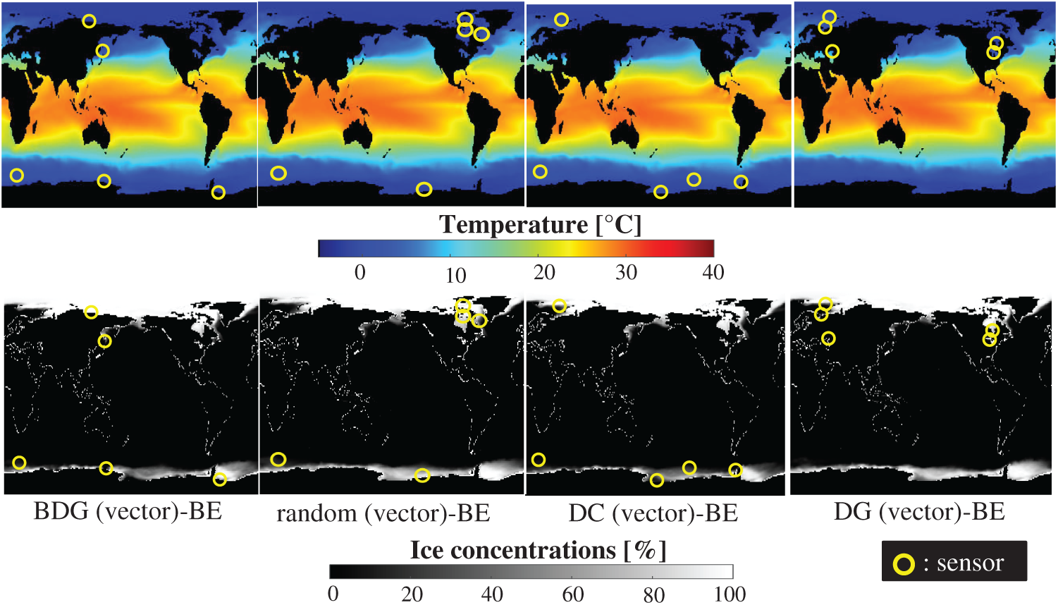
Figure 22: Single snapshots of the original data and reconstructed fields data by the BDG (vector)-BE, random (vector)-BE, DC (vector)-BE and DG (vector)-BE methods, respectively in the NOAA-SST/ICEC problem: n = 88438, m = 520, r = 10, p = 5, and s = 2

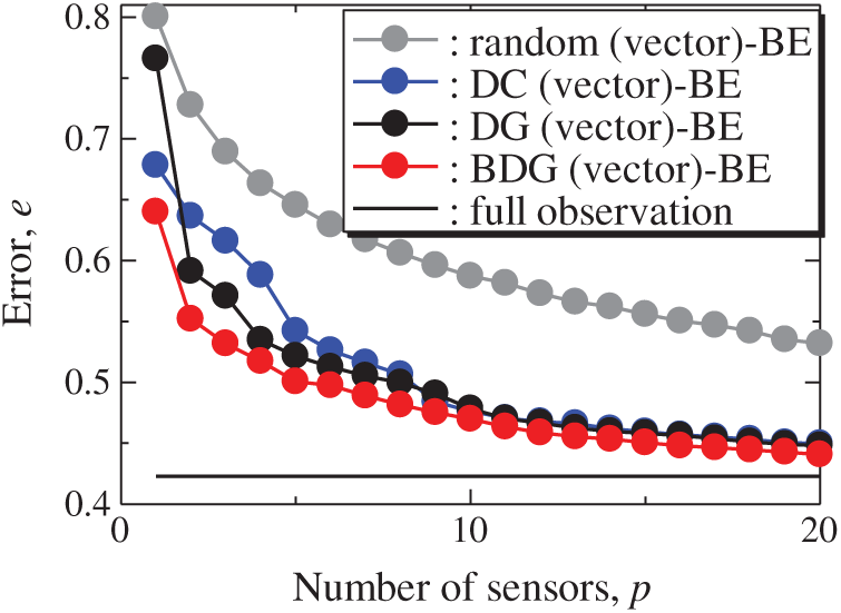
Figure 23: Errors of the results using the random (vector)-BE, DC (vector)-BE, DG (vector)-BE and BDG (vector)-BE methods against the number of sensors in the NOAA-SST/ICEC problem: n = 88438, m = 520, r = 10, and s = 2

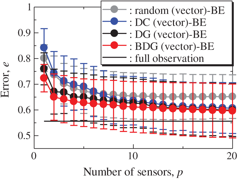
Figure 24: Errors of the K-fold cross-validation results using the random (vector)-BE, DC (vector)-BE, DG (vector)-BE and BDG (vector)-BE methods against the number of sensors in the NOAA-SST/ICEC problem: n = 88438, m = 520, r = 10, s = 2, and K = 5

All the errors estimated by the BE method are smaller than those estimated by the LSE method as shown in Figs. 20 and 21, and monotonically decrease as the number of sensors increases as well as the problems of the random sensor and PIV. The error of the BDG (vector)-BE method, which extended to the vector-sensor measurement in the present study is the smallest in the NOAA/ICEC problem. There is a larger difference between the upper and lower bounds of the error bars than the ones in the PIV problem shown in Fig. 14. The error of the BDG (vector)-BE, which is extended to the vector-sensor measurement in the present study, is the smallest in the NOAA-SST/ICEC problem although the large difference of the error bars might implicate that the quantitative performance of the proposed methods depends on the problem. Fig. 25 shows the relationship between the computational time and the number of sensors p in the NOAA-SST/ICEC problem. Note that, the locations are beforehand excluded from S for simplicity if their RMSs are 10−1 times smaller than the maximum of the NOAA-SST/ICEC dataset, and S¯ denotes a subset of S after this exclusion in the NOAA-SST/ICEC problem. Therefore, the actual n is smaller than the initial n = 88438. The random (vector) and DC (vector) methods take a certain amount of time regardless of the number of sensors. The computational times of the DG (vector) and BDG (vector) methods increase monotonically as the number of sensors increases since the sensors are determined greedily. The computational time of the BDG (vector) method is shorter than that of the DC (vector) method, and the BDG (vector) method has the smallest error in the NOAA-SST/ICEC problem as shown in Figs. 23 and 24. In addition, the r2 truncation [24] for the BDG (vector) method will reduce the computational time although the r2 truncation is not addressed in the NOAA-SST/ICEC problem. The DG (vector) method, which has the same error as the DC (vector) method, is faster than the BDG (vector) and DC (vector) methods in this NOAA-SST/ICEC problem. Therefore, the BDG (vector) and DG (vector) methods extended in the present study are better methods in the NOAA-SST/ICEC problem.

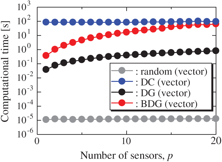
Figure 25: Computational times of the results using the random (vector), DC (vector), DG (vector), and BDG (vector) methods against the number of sensors in the NOAA-SST/ICEC problem: n = 88438, m = 520, r = 10, s = 2, and K = 5

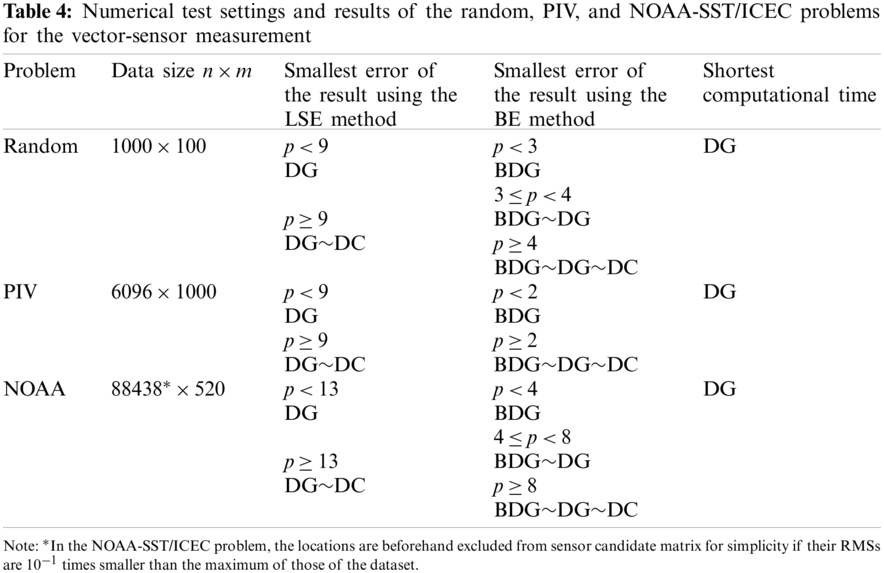
Tab. 4 summarizes the numerical test settings and results of the random, PIV, and NOAA-SST/ICEC problems for the vector-sensor measurement. Here, all the methods excluding the random method are compared. The trends of the errors and computational time are the same in all problems in the present study. The errors of the results using the DG (vector)-LSE and BDG (vector)-BE methods are the smallest for all problems. In addition, as the number of sensors increases, the errors of the results using the DC (vector)-LSE is close to that of the results using the DG (vector)-LSE method, and the error of the results using DG (vector)-BE and DC (vector)-BE methods is close to that of the BDG (vector)-BE method. The computational time of the DG (vector) method is the shortest for all problems. These results summarize that the proposed DG (vector) and BDG (vector) methods extended to the vector-sensor measurement are superior to the random (vector) and DC (vector) methods in terms of the accuracy of the sensor selection and computational cost in the present study.

4  Conclusions

A vector-measurement-sensor-selection problem in the under and oversampled cases is considered by extending the previous novel approaches: a greedy method based on D-optimality (DG) and a noise-robust greedy method (BDG) in the present study. Extensions of the vector-measurement-sensor selection of the greedy algorithms are proposed and applied to randomly generated systems and practical datasets of flowfield around airfoil and global climates and the full states are reconstructed by the vector-sensor measurement. In all demonstrations, the random selection and convex approximation methods are evaluated as the references in addition to the proposed DG and BDG methods. The least squares and Bayesian estimation methods are employed as the state estimation method in the present study.

The results applied to randomly generated systems show the proposed DG and BDG methods select better the position of the sparse sensor than the random selection and convex approximation methods. The results applied to practical datasets of flowfield around the airfoil and global climates are similar to the results applied to randomly generated systems. In addition, the reconstructed fields from the selected sensor in the noise-robust greedy (BDG) method are closest to the original data in all demonstrations. These results illustrate that the proposed methods extended to the vector-sensor measurement are superior to the random selection and convex approximation methods in terms of the accuracy of the sensor selection and computational cost in the present study.

Although the vector-measurement-sensor-selection problem extended by the present study is a more realistic sensor placement problem than the traditional scalar-measurement-sensor-selection problem, there are gaps between ideal models and real-world practicalities. For example, which is the better whether to place a large number of cheap sensors having a low signal-to-noise level, a small number of expensive sensors having a high signal-to-noise level, or a mix of both. The sensor selection problem considering the cost problem [17–19] will be the subject of challenging future research.

Funding Statement: This work was supported by JST ACT-X (JPMJAX20AD), JST CREST (JPMJCR1763) and JST FOREST (JPMJFR202C), Japan.

Conflicts of Interest: The authors declare that they have no conflicts of interest to report regarding the present study.

References

 1.  Berkooz, G., Holmes, P., Lumley, J. L. (1993). The proper orthogonal decomposition in the analysis of turbulent flows. Annual Review of Fluid Mechanics, 25(1), 539–575. DOI 10.1146/annurev.fl.25.010193.002543. [Google Scholar] [CrossRef]

 2.  Taira, K., Brunton, S. L., Dawson, S. T., Rowley, C. W., Colonius, T. et al. (2017). Modal analysis of fluid flows: An overview. AIAA Journal, 55(12), 4013–4041. DOI 10.2514/1.J056060. [Google Scholar] [CrossRef]

 3.  Schmid, P. J. (2010). Dynamic mode decomposition of numerical and experimental data. Journal of Fluid Mechanics, 656, 5–28. DOI 10.1017/S0022112010001217. [Google Scholar] [CrossRef]

 4.  Kutz, J. N., Brunton, S. L., Brunton, B. W., Proctor, J. L. (2016). Dynamic mode decomposition: Data-driven modeling of complex systems. USA: Society for Industrial and Applied Mathematics. [Google Scholar]

 5.  Nonomura, T., Shibata, H., Takaki, R. (2018). Dynamic mode decomposition using a kalman filter for parameter estimation. AIP Advances, 8(10), 105106. DOI 10.1063/1.5031816. [Google Scholar] [CrossRef]

 6.  Nonomura, T., Shibata, H., Takaki, R. (2019). Extended-Kalman-filter-based dynamic mode decomposition for simultaneous system identification and denoising. PLoS One, 14(2), e0209836. DOI 10.1371/journal.pone.0209836. [Google Scholar] [CrossRef]

 7.  Manohar, K., Brunton, B. W., Kutz, J. N., Brunton, S. L. (2018). Data-driven sparse sensor placement for reconstruction: Demonstrating the benefits of exploiting known patterns. IEEE Control Systems Magazine, 38(3), 63–86. DOI 10.1109/MCS.2018.2810460. [Google Scholar] [CrossRef]

 8.  Joshi, S., Boyd, S. (2009). Sensor selection via convex optimization. IEEE Transactions on Signal Processing, 57(2), 451–462. DOI 10.1109/TSP.2008.2007095. [Google Scholar] [CrossRef]

 9.  Nonomura, T., Ono, S., Nakai, K., Saito, Y. (2021). Randomized subspace newton convex method applied to data-driven sensor selection problem. IEEE Signal Processing Letters, 28, 284–288. DOI 10.1109/LSP.2021.3050708. [Google Scholar] [CrossRef]

10. Nagata, T., Nonomura, T., Nakai, K., Yamada, K., Saito, Y. et al. (2021). Data-driven sparse sensor selection based on A-optimal design of experiment with ADMM. IEEE Sensors Journal, 21(13), 15248–15257. DOI 10.1109/JSEN.2021.3073978. [Google Scholar] [CrossRef]

11. Chaturantabut, S., Sorensen, D. C. (2010). Nonlinear model reduction via discrete empirical interpolation. SIAM Journal on Scientific Computing, 32(5), 2737–2764. DOI 10.1137/090766498. [Google Scholar] [CrossRef]

12. Drmac, Z., Gugercin, S. (2016). A new selection operator for the discrete empirical interpolation method–improved a priori error bound and extensions. SIAM Journal on Scientific Computing, 38(2), A631–A648. DOI 10.1137/15M1019271. [Google Scholar] [CrossRef]

13. Peherstorfer, B., Drmac, Z., Gugercin, S. (2020). Stability of discrete empirical interpolation and gappy proper orthogonal decomposition with randomized and deterministic sampling points. SIAM Journal on Scientific Computing, 42(5), A2837–A2864. DOI 10.1137/19M1307391. [Google Scholar] [CrossRef]

14. Astrid, P., Weiland, S., Willcox, K., Backx, T. (2008). Missing point estimation in models described by proper orthogonal decomposition. IEEE Transactions on Automatic Control, 53(10), 2237–2251. DOI 10.1109/TAC.2008.2006102. [Google Scholar] [CrossRef]

15. Barrault, M., Maday, Y., Nguyen, N. C., Patera, A. T. (2004). An ‘empirical interpolation’ method: Application to efficient reduced-basis discretization of partial differential equations. Comptes Rendus Mathematique, 339(9), 667–672. DOI 10.1016/j.crma.2004.08.006. [Google Scholar] [CrossRef]

16. Carlberg, K., Farhat, C., Cortial, J., Amsallem, D. (2013). The gnat method for nonlinear model reduction: Effective implementation and application to computational fluid dynamics and turbulent flows. Journal of Computational Physics, 242, 623–647. DOI 10.1016/j.jcp.2013.02.028. [Google Scholar] [CrossRef]

17. Clark, E., Askham, T., Brunton, S. L., Kutz, J. N. (2018). Greedy sensor placement with cost constraints. IEEE Sensors Journal, 19(7), 2642–2656. DOI 10.1109/JSEN.2018.2887044. [Google Scholar] [CrossRef]

18. Clark, E., Kutz, J. N., Brunton, S. L. (2020). Sensor selection with cost constraints for dynamically relevant bases. IEEE Sensors Journal, 20(19), 11674–11687. DOI 10.1109/JSEN.2020.2997298. [Google Scholar] [CrossRef]

19. Clark, E., Brunton, S. L., Kutz, J. N. (2021). Multi-fidelity sensor selection: Greedy algorithms to place cheap and expensive sensors with cost constraints. IEEE Sensors Journal, 21(1), 600–611. DOI 10.1109/JSEN.2020.3013094. [Google Scholar] [CrossRef]

20. Manohar, K., Kutz, J. N., Brunton, S. L. (2018). Optimal sensor and actuator selection using balanced model reduction. arXiv preprint arXiv: 1812.01574. [Google Scholar]

21. Saito, Y., Nonomura, T., Yamada, K., Nakai, K., Nagata, T. et al. (2021). Determinant-based fast greedy sensor selection algorithm. IEEE Access, 9, 68535–68551. DOI 10.1109/ACCESS.2021.3076186. [Google Scholar] [CrossRef]

22. Shamaiah, M., Banerjee, S., Vikalo, H. (2010). Greedy sensor selection: Leveraging submodularity. 49th IEEE Conference on Decision and Control, pp. 2572–2577. Atlanta, GA, USA, IEEE. DOI 10.1109/CDC.2010.5717225. [Google Scholar] [CrossRef]

23. Nakai, K., Yamada, K., Nagata, T., Saito, Y., Nonomura, T. (2021). Effect of objective function on data-driven greedy sparse sensor optimization. IEEE Access, 9, 46731–46743. DOI http://dx.doi.org/10.1109/ACCESS.2021.3067712. [Google Scholar] [CrossRef]

24. Yamada, K., Saito, Y., Nankai, K., Nonomura, T., Asai, K. et al. (2021). Fast greedy optimization of sensor selection in measurement with correlated noise. Mechanical Systems and Signal Processing, 158(6), 107619. DOI 10.1016/j.ymssp.2021.107619. [Google Scholar] [CrossRef]

25. Inoue, T., Matsuda, Y., Ikami, T., Nonomura, T., Egami, Y. et al. (2021). Data-driven approach for noise reduction in pressure-sensitive paint data based on modal expansion and time-series data at optimally placed points. Physics of Fluids, 33(7), 77105. DOI 10.1063/5.0049071. [Google Scholar] [CrossRef]

26. Kaneko, S., Ozawa, Y., Nakai, K., Saito, Y., Nonomura, T. et al. (2021). Data-driven sparse sampling for reconstruction of acoustic-wave characteristics used in aeroacoustic beamforming. Applied Sciences, 11(9), 4216. DOI 10.3390/app11094216. [Google Scholar] [CrossRef]

27. Kanda, N., Nakai, K., Saito, Y., Nonomura, T., Asai, K. (2021). Feasibility study on real-time observation of flow velocity field by sparse processing particle image velocimetry. Transactions of the Japan Society for Aeronautical and Space Sciences, 64(4), 242–245. DOI 10.2322/tjsass.64.242. [Google Scholar] [CrossRef]

28. Saito, Y., Nonomura, T., Nankai, K., Yamada, K., Asai, K. et al. (2020). Data-driven vector-measurement-sensor selection based on greedy algorithm. IEEE Sensors Letters, 4, 7002604. DOI 10.1109/LSENS.2020.2999186. [Google Scholar] [CrossRef]

29. Horn, R. A., Johnson, C. R. (2012). Matrix analysis. UK: Cambridge University Press. [Google Scholar]

30. Anderson, M., Ballard, G., Demmel, J., Keutzer, K. (2011). Communication-avoiding QR decomposition for GPUs. 2011 IEEE International Parallel & Distributed Processing Symposium, pp. 48–58. Anchorage, AK, USA, IEEE. DOI 10.1109/IPDPS.2011.15. [Google Scholar] [CrossRef]

31. Nankai, K., Ozawa, Y., Nonomura, T., Asai, K. (2019). Linear reduced-order model based on PIV data of flow field around airfoil. Transactions of the Japan Society for Aeronautical and Space Sciences, 62(4), 227–235. DOI 10.2322/tjsass.62.227. [Google Scholar] [CrossRef]

32. Loiseau, J. C., Noack, B. R., Brunton, S. L. (2018). Sparse reduced-order modelling: Sensor-based dynamics to full-state estimation. Journal of Fluid Mechanics, 844, 459–490. DOI 10.1017/jfm.2018.147. [Google Scholar] [CrossRef]

33. NOAA/OAR/ESRL Physical Sciences Laboratory (2019). NOAA optimum interpolation (OI) sea surface temperature (SST) V2. https://psl.noaa.gov/data/gridded/data.noaa.oisst.v2.html. [Google Scholar]

This work is licensed under a Creative Commons Attribution 4.0 International License, which permits unrestricted use, distribution, and reproduction in any medium, provided the original work is properly cited.