Computer Modeling in Engineering & Sciences

DOI: 10.32604/cmes.2021.016050

ARTICLE

A 3-Node Co-Rotational Triangular Finite Element for Non-Smooth, Folded and Multi-Shell Laminated Composite Structures

Zhongxue Li1,*, Jiawei Ji1, Loc Vu-Quoc2, Bassam A. Izzuddin3 and Xin Zhuo1

1Department of Civil Engineering, Zhejiang University, Hangzhou, 310058, China
2Aerospace Engineering, University of Illinois at Urbana-Champaign, Urbana, IL 61801, USA
3Department of Civil and Environmental Engineering, Imperial College London, London, SW7 2BU, UK
*Corresponding Author: Zhongxue Li. Email: lizx19993@zju.edu.cnEmails: lizx19993@zju.edu.cn, 21812040@zju.edu.cn, vql@illinois.edu, b.izzuddin@imperial.ac.uk, zhuoxin@zju.edu.cn
Received: 02 February 2021; Accepted: 06 July 2021

1  Introduction

Laminated composite shell structures are extensively used in pressure vessels, aircraft and spacecraft, automotive and other industries due to their high strength- and stiffness-to-mass ratios, excellent damage tolerance, superior fatigue response characteristics, and good damping behaviors under dynamic loads. By choosing an appropriate combination of reinforcement and matrix material, manufacturers can produce properties that exactly fit the requirements of a particular structure design [1]. The mechanical properties of laminated composite structures are sensitive to the lamination scheme and the ply orientation angle, so they often show unique responses even under simple loading conditions and geometric configurations. Furthermore, the anisotropic constitutive responses and the complexity of shell geometries, such as non-smooth and folded shell structures, make it challenging to perform accurate structural analysis, especially when large deformations are involved. Therefore, the development of reliable and efficient finite element methods for laminated composite shell structures are important [1–5].

Various computational formulations have been proposed for modeling composite shells and plates, and can be broadly classified into three categories: (1) single-director theories with anisotropic constitutive relations and (2) multi-director theories, which include multi-layer formulations, within which each layer has a single director with its own anisotropic constitutive relation, and (3) 3-D continuum theories. Examples of single-director theories include the classical laminated plate/shell theory (CLPT), the first-order shear deformation laminated plate/shell theory (FSDT), and the higher-order shear deformation laminated plate/shell theories (HSDT). Examples of multi-director theories include the layer-wise theory (LWT) and the zig-zag theory (ZZT). Examples of 3-D continuum theories include solid-shell formulations with a single layer or a multilayer structure.

In the single-director category, the CLPT is restricted to thin shell structures, as the effects of transverse shear strains and thickness strains are ignored. Based on the CLPT, Madenci et al. [6] proposed a free-formulation-based 3-node flat triangular shell element for geometrically nonlinear analysis of thin composite shells. Kapania et al. [7] presented a 3-node triangular flat shell element by combining a discrete Kirchhoff plate bending element with a membrane element for linear static, free vibration and thermal analysis of laminated plates and shells. Bisegna et al. [8] proposed a co-rotational triangular facet shell element for geometric nonlinear analysis of thin piezo-actuated structures.

Also in the single-director category, under the FSDT, the transverse shear strains are assumed to remain constant through the thickness, and the shell normal does not need to remain perpendicular to the mid-surface after deformation, while the inextensibility of transverse shell normal is assumed. Based on this theory, Peng et al. [9] proposed a meshfree method for bending analysis of folded laminated plates. Pham et al. [10] presented a combination of the edge-based smoothed finite element method (ES-FEM) and the three-node triangular elements (MITC3) for static responses and free vibration of laminated composite shells. Truong-Thi et al. [11] presented an extension of the cell-based smoothed discrete shear gap method using three-node triangular elements for the static and free vibration analyses of carbon nano-tube reinforced composite plates. Zhang et al. [12,13] developed an eight-node quadrilateral plate element with five mechanical degrees of freedom and one electric degree of freedom for static and dynamic analyses of piezoelectric integrated carbon nanotube reinforced functionally graded composite structures. Kreja et al. [14] presented isoparametric eight-node Serendipity-type shell finite elements to check the relevance of five- and six-parameter variants for large rotation plate and shell problems. The FSDT provides a balance between computational efficiency and accuracy for the global structural behaviors of thin and moderately thick laminated composite shells, while the local effects (e.g., inter-laminar stress distribution between layers, delamination, etc.) are often difficult to capture.

The HSDT provides a more accurate description of the transverse shear stress distributions by introducing more independent displacement parameters. Within the HSDT, Chen et al. [15] presented a refined three-node triangular element satisfying the requirement of C1 weak-continuity. Tran et al. [16,17] proposed an edge-based smoothing discrete shear gap method using 3-node triangular elements combined with a C0-type higher-order shear deformation theory for static, free vibration and buckling analyses of laminated composite plates. Jin et al. [18] proposed a computationally efficient C0-type 3-node triangular plate element with linear interpolation functions for the analysis of multi-layered composite plates based on the mixed global-local higher-order theory.

In the multi-director category, the LWT assumes a layer-wise deformation pattern, and it can predict the interlaminar stresses accurately. Liu et al. [19] employed a layer-wise three-node triangular shell element for modeling the opening and shear modes of delamination. Phung-Van et al. [20] presented an extension of the cell-based smoothed discrete shear gap method using three-node triangular elements for dynamic responses of sandwich and laminated composite plates. Marjanović et al. [21] presented a triangular layered finite element with delamination degrees of freedom for composite shells based on the generalized LWT. For large deformation and large overall motion, Vu-Quoc et al. [22,23] developed the dynamic formulations for geometrically-exact multilayered composite beams, plates, and shells with ply drop-offs. However, layer-wise models are computationally expensive since the number of unknowns depends on the number of the layers of the laminates.

The ZZT describes a piecewise continuous displacement field in the plate thickness direction and fulfills interlaminar continuity of transverse stresses at each layer interface. Carrera [24] provides a comprehensive review of the ZZT. Versino et al. [25] developed six- and three-node triangular plate elements for homogeneous, multilayer composite and sandwich plates based on the refined zigzag theory. Nguyen et al. [26] developed a three-node triangular finite element for visco-elastic composite laminates based on a high-order zigzag theory. Wu et al. [27] proposed an efficient three-node triangular element with linear shape functions to model sandwich plates based on the refined higher-order zig-zag model in conjunction with the three-field Hu–Washizu variational principle. Liang et al. [28,29] proposed an efficient zigzag kinematic model for composite laminates with multiple alternating stiff-soft layers, which has been realized within a corotational shell element utilizing additional zigzag DOFs that are not subject to the corotational transformations, making use of a 2D local shell system over the surface of the structure.

The 3D continuum-based theory accounts for fully 3D constitutive behaviors, so the interlaminar stress of composite laminates can be effectively captured. Houmat [30] studied the free vibration of variable stiffness laminated composite plates using the 3D elasticity theory and the p-version finite element method. Ye et al. [31] used the scaled boundary finite element method to analyze the bending behaviors of the angle-ply composite laminated cylindrical shells based on 3D theory of elasticity. Kumari et al. [32] adopted the Reissner variational principle and the extended Kantorovich method to study the bending problem of composite cylindrical shells with arbitrarily support boundary conditions. Vu-Quoc et al. [33] developed multilayered composite solid-shell formulations, for both static and dynamic analyses, that could accommodate 3-D constitutive relations without a need to impose zero transverse normal stresses. Fan et al. [34] developed lowest-order (8-node hexahedral), and higher-order (32-node hexahedral) 3-D continuum solid-shell elements, based on the theory of 3D solid mechanics, for static and dynamic analyses of composite laminates.

Despite these developments, numerical formulations based on the theories of HSDT, LWT, ZZT and 3D continuum-based theory often lead to high computational costs, which is a major concern in their practical applications. In the present study, a 3-node co-rotational triangular composite shell finite element is developed based on FSDT, where vectorial rotational variables are employed as rotational variables, two smaller components of one vector, together with the smallest or second smallest component of another vector, of an orthogonal triad initially oriented along the global coordinate system axes at each node on a non-smooth intersection of plates and/or shells are defined as vectorial rotational variables, while two smaller components of the mid-surface normal vector of shell at other nodes are defined as vectorial rotational variables. The resulting element tangent stiffness matrices are symmetric owing to the commutativity of nodal variables in calculating the second derivatives of strain energy with respect to local nodal variables and the second derivatives of the local nodal variables with respect to global nodal variables. Using such vectorial rotational variables, triangular and quadrilateral shell elements have been developed for large displacement and large rotation analyses of smooth shell structures [35–38], as well as non-smooth shells made of isotropic elastic materials [39,40]. The 3-node finite element formulation proposed in the present study is capable of modeling both smooth and non-smooth laminated composite shell structures experiencing large deformations.

There have been continuous efforts in developing triangular shell finite elements with high computational accuracy and convergence [41,42]. It is well-known that triangular finite elements may suffer from locking phenomena with thin shell/plate thickness, which results in the deterioration of computational accuracy and convergence. Up to now, there is no optimal 3-node triangular shell element, the main reason is that the strain distributions derived from displacement shape functions are often wildly different than expected. Barlow points, at which the strains derived from displacement shape functions are “correct” for all desired deformation modes and all permitted initial element shapes, can be found in a quadrilateral element, and they can be employed in calculating the element tangent stiffness matrix to eliminate locking phenomena. There exist no Barlow points, however, in a triangular shell element, thus there is no set of integration points that provides zero membrane strain for all cases of pure bending about axes parallel to each of the three edges of a triangular element. Most methods for eliminating locking problems of quadrilateral shell elements do not work well in triangular elements, such as reduced integration technique [43] and Hellinger-Reissner mixed formula method [44]. Macneal [45] proposed a line integration method to overcome locking problems, where assumed membrane strains and assumed shear strains are calculated respectively from the edge member membrane strains and the edge member transverse shear strains. Bletzinger [46] presented a discrete shear gap method (DSG) which utilizes only the usual displacement and rotational degrees of freedom at the nodes. Kim et al. [47] developed a 3-node macro triangular element using assumed natural strain method (ANS) for geometrically non-linear analysis of plates and shells. The ANS formula and the macro element strategy can reduce the locking effect and preserve its advantages in preprocessing. Argyris et al. [48,49] proposed a facet triangular shell element (TRIC) for nonlinear dynamic and elasto-plastic shell analyses using the natural mode method. Lee et al. [50] presented a Mixed Interpolation of Tensorial Components approach (MITC) for shell elements, which have been extended to MITC3 and MITC3+ shell finite elements by introducing interpolation cover functions and cubic bubble function for the rotations [51,52]. Cai et al. [53] proposed a locking-free discrete shear triangular plate element without any numerical expediencies such as the reduce integration and assumed strains method. In the present study, transverse shear strains of the shell finite element are replaced with assumed shear strains obtained using the line integration approach [35,45] to overcome shear locking.

The outline of the paper is as follows. Section 2 describes the co-rotational framework and the kinematics of the 3-node triangular composite shell element. Section 3 presents the composite shell finite element formulation in the co-rotational local co-ordinate system. Section 4 gives the transformation relationship between the local and global responses. Several numerical examples are analyzed in Section 5 to verify the numerical accuracy of the present finite element. Conclusions are presented in Section 6.

2  Co-Rotational Framework and Kinematics of the 3-Node Shell Finite Element

2.1 Co-Rotational Framework

The co-rotational framework for the 3-node shell finite element is depicted in Fig. 1. The origin of the local co-rotational coordinate system of the element coincides with Node 1 in the initial configuration, and the coordinate system rotates with the element's rigid body rotation, but does not deform with the element. Although the adopted definition is not invariant to nodal ordering [54], the associated variability is negligible for large-displacement small strain problems. To define the local system, we firstly calculate the vectors v120 and v130:

v120=X20−X10,v130=X30−X10(1a,b)

where Xi0 (i = 1, 2, 3) is the position of Node i in the initial global coordinate system. The base vectors of the local coordinate system in the initial configuration are calculated as follows:

ex0=v120|v120|,ez0=v120×v130|v120×v130|,ey0=ez0×ex0(2a,b,c)

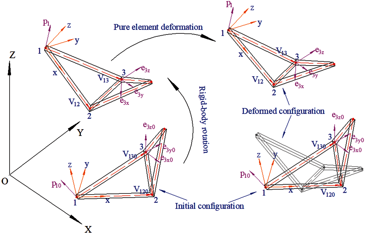
Figure 1: Illustration of the co-rotational framework

In the deformed configuration, the vectors v12 and v13 are defined as

v12=X20−X10+d2−d1,v13=X30−X10+d3−d1(3a,b)

where di (i = 1, 2, 3) is the translational displacement vector of Node i in the global coordinate system. Accordingly, the base vectors of the current local coordinate system can be obtained

ex=v12|v12|,ez=v12×v13|v12×v13|,ey=ez×ex(4a,b,c)

In the global coordinate system, we define the following vector that consists of all the global DOFs (degrees of freedom) for each element:

uGT=⟨d1Tng1Td2Tng2Td3Tng3T⟩(5)

where diT=⟨UiViWi⟩ are three translational displacement DOFs of Node i, and ngiT denotes the vectorial rotational DOFs of Node i. For any node of smooth shells or located away from non-smooth shells intersections, ngiT=⟨pi,npi,m⟩ is defined to represent the vectorial rotational DOFs, in which pi,n and pi,m denote the two smaller global components of the shell director pi. The remaining component of the shell director pi is defined as

pi,l=s41−pi,n2−pi,m2,i=1,2,3(6)

where s4=±1 takes the same sign as that of pi,l in the previous loading step, and {n, m, l} denotes the circular permutation of {X, Y, Z}.

On the other hand, if Node i is located on the intersections of non-smooth shells, the vectorial rotational DOFs of Node i is defined as ngiT=⟨eiy,neiy,meiz,n⟩. Here, eiy,n and eiy,m are the two smaller components of eiy, and eiz,n is the smallest or second smallest component of eiz, where eiy and eiz are two orientation vectors of an orthogonal triad at Node i. At each incremental loading step, the following relationships can be derived:

‖eiy‖2=eiy,l2+eiy,m2+eiy,n2=1⇒eiy,l=s11−(eiy,m2+eiy,n2)(7)

‖eiz‖2=eiz,l2+eiz,m2+eiz,n2=1⇒eiz,m=s31−(eiz,n2+eiz,l2)(7b)

‖eiy‖2=1‖eiz‖2=1eiyTeiz=0}⇒eiz,l=−eiy,leiy,neiz,n+s2eiy,m1−eiy,n2−eiz,n21−eiy,n2(7c)

The remaining components of the vectors eiy and eiz can be calculated by using eiy,n, eiy,m and eiz,n according to Eqs. (7a)–(7c). The sign symbols (s1,s3) defined as 1 or −1 are respectively equal to the signs of components eiy,l and eiz,m of the last incremental step, and we have s2=−s1⋅s3. The vector eix is calculated as the cross-product of eiy and eiz:

eix=eiy×eiz(8)

Since the norm of a unit vector is identical to 1, defining the vectorial rotational variables as above can avoid ill-conditioning in updating the mid-surface normal vector at a node on the smooth part of the plate or shell (away from non-smooth intersections) or orientation vectors of an orthogonal triad at a node on a non-smooth intersection of plates or shells by properly controlling the size of loading step in a nonlinear incremental solution procedure.

There are 15 degrees of freedom per element in the local coordinate system

uLT=⟨t1Tθ1Tt2Tθ2Tt3Tθ3T⟩(9)

where tiT=⟨ui vi wi⟩ are three translational displacement components, θiT=⟨ri,x ri,y⟩ are vectorial rotational components, ri,x and ri,y are the components of the shell director at Node i along the x-axis and y-axis directions in the local coordinate system.

The relationship between the local and global translational displacements can be expressed as follows:

ti=R(di+vi0)−R0vi0(10)

where,

R0T=[ex0ey0ez0],RT=[exeyez](11)

vi0=Xi0−X10,i=1,2,3(12)

At any node of smooth shells or any node away from non-smooth shell intersections, the relationship between the shell directors expressed in the local and global coordinate systems can be described as

ri0=R0pi0,ri=Rpi(13)

At any node on intersections of non-smooth shells, the following relationships between the shell directors in the local and global coordinate systems hold:

ri0=R0Ri0TRi0pi0=R0pi0,ri=RRiTRi0pi0(14)

where

Ri0T=[eix0eiy0eiz0],RiT=[eixeiyeiz](15a,b)

For convenience, eix0,eiy0 and eiz0 in the initial configuration are chosen to be coincident with the base vectors of the global coordinate system.

eix0T=⟨100⟩,eiy0T=⟨010⟩,eiz0T=⟨001⟩(16a,b,c)

2.2 Description of the Element Geometry and Kinematics

The finite element shape functions are expressed in the natural coordinate system as follows:

N1=1−ξ−η,N2=ξ,N3=η(17a,b,c)

The displacement at any point of the element is calculated as follows:

t=⟨uvw⟩T=∑i=13Ni[ti+12ζa(ri−ri0)](18)

In the initial configuration, the shell director at Node i is calculated as the cross product of the tangent vectors along two natural coordinate axes.

p¯i0=∂X0∂ξ×∂X0∂η|(ξi,ηi),i=1,2,3(19)

where

X0=∑i=13Ni(ξ,η)Xi0(20)

To ensure the uniqueness of the shell director at any node shared by multiple adjacent elements in smooth shell regions, the following averaging procedure is adopted:

pi0=∑e∈Sip¯i0e/‖p¯i0e‖‖∑e∈Sip¯i0e/‖p¯i0e‖‖(21)

The Green–Lagrange strain of the nonlinear shallow shell theory is adopted. For convenience, the strain vector is divided into membrane strain vector εm, bending strain vector zlχ and transverse shear strain vector γ.

ε={εm+zlχγ}(22a)

εmT=⟨εxxεyyγxy⟩=⟨∂u∂x∂υ∂y∂u∂y+∂υ∂x⟩(22b)

χT=⟨∂(rx−rx0)∂x∂(ry−ry0)∂y∂(rx−rx0)∂y+∂(ry−ry0)∂x⟩(22c)

γT=⟨γxzγyz⟩=⟨∂w∂x+rx−rx0∂w∂y+ry−ry0⟩(22d)

zl=12ζa(22e)

where, zl is the coordinate of the material point along the shell thickness direction, a is the thickness of the element, and

rx0=∑i=13Niri0,x,rx=∑i=13Niri,x,ry0=∑i=13Niri0,y,ry=∑i=13Niri,y(23a,b,c,d)

3  Laminated Composite Shell Finite Element Formulation in the Co-Rotational Local Coordinate System

The potential energy of a 3-node triangular composite shell finite element is defined as

Π=12∫V{εm+zlχγ}TC{εm+zlχγ}dV−We(24)

where We is the work done by the external load, C is the elastic constitutive matrix. In the present study, we consider a laminated shell structure composed of long-fiber-reinforced materials. The transversely isotropic elastic constitutive matrix of each individual lamina is expressed in the material coordinate system as

C=[E11−μ12μ21μ12E21−μ12μ21000μ12E21−μ12μ21E21−μ12μ2100000G120000G1300000G23](25)

where, μ12 and μ21 are the Poisson's ratios, E1 and E2 are the elastic moduli, G12, G23 and G31 are the shear moduli [1,14].

By enforcing the stationarity condition to the potential energy, we have

δΠ=12∫V{εm+zlχγ}TC[Bm+zlBbBγ]δuLdV−δWe=0(26)

which yields the element internal force vector:

fint=fext=12∫V[Bm+zlBbBγ]TC{εm+zlχγ}dV(27)

where uL, fext and fint are element nodal displacement vector, external load vector and internal force vector in the co-rotational local coordinate system, respectively. Bm, Bb and Bγ contain the first-order derivatives of the membrane strain, bending strain, and shear strain, respectively. Details of these matrices are given in Appendix A.

By taking the first-order derivative of the internal force vector with respect to the local nodal variables, a symmetric element tangent stiffness matrix is obtained

kT=∫V[Bm+zlBbBγ]TC[Bm+zlBbBγ]dV(28)

For elastic laminated shell elements, the integration along the shell thickness direction is decoupled from the integration on the mid-surface, so Eqs. (27) and (28) involving volume integrals can be rewritten in the following surface integral form:

fint=a2∫A[BmBγ]TDeq1{εmγ}dA+a324∫A[Bb0]TDeq2{χ0}dA+a28∫A([BmBγ]TDeq3{χ0}+[Bb0]TDeq3{εmγ})dA(29)

kT=a2∫A[BmBγ]TDeq1[BmBγ]dA+a324∫A[Bb0]TDeq2[Bb0]dA+a28∫A([BmBγ]TDeq3[Bb0]+[Bb0]TDeq3[BmBγ])dA(30)

where Deq1, Deq2 and Deq3 are the equivalent elastic matrices:

Deq1=∑i=1n(ζi+1−ζi)Dci,Deq2=∑i=1n(ζi+13−ζi3)Dci,Deq3=∑i=1n(ζi+12−ζi2)Dci(31a,b,c)

n denotes the number of laminae; ζi is the dimensionless coordinate of the interface between Layer i−1 and Layer i relative to the mid-surface:

ζi=−1.0+2n(i−1),i=1,2,…,n,(32)

Dci is the elastic matrix of the ith layer lamina:

Dci=TiTCiTi(33)

where Ci is the transversely isotropic elastic matrix of Layer i in the material coordinate system, which is obtained by replacing the material properties of Eq.(25) with those of the ith layer; Ti is the transformation matrix between the material coordinate system of the ith layer lamina and the co-rotational element local coordinate system:

Ti=[cos2φisin2φi12sin⁡2φi00sin2φicos2φi−12sin⁡2φi00−sin⁡2φisin⁡2φicos⁡2φi00000cos⁡φisin⁡φi000−sin⁡φicos⁡φi](34)

where φi is defined as the ply orientation angle measured between the reinforcement fiber of the ith layer lamina and the co-rotational local coordinate system of the composite element. It is noted that, for symmetrical laminates, the third integrals of Eqs. (29) and (30) are equal to zero.

To alleviate shear locking phenomenon, the assumed transverse shear strain vector and its first-order derivatives with respect to local nodal variables are employed. The modified line integration approach [35,45] is adopted to calculate the assumed shear strains, and by replacing the conforming transverse shear strain and its first-order derivatives with the assumed strains and its first-order derivatives with respect to local nodal variables, the following assumed strain finite element formulation is obtained:

fint=h2∫A[BmB~γ]TDeq1{εmγ~}dA+h324∫A[Bb0]TDeq2{χ0}dA+h28∫A([BmB~γ]TDeq3{χ0}+[Bb0]TDeq3{εmγ~})dA (35)

kT=h2∫A[BmB~γ]TDeq1[BmB~γ]dA+h324∫A[Bb0]TDeq2[Bb0]dA+h28∫A([BmB~γ]TDeq3[Bb0]+[Bb0]TDeq3[BmB~γ])dA (36)

where γ~ is the assumed transverse shear strain vector, B~γ is its first-order derivative with respect to local nodal variables uL (refer to Eqs. (30)–(41) in reference [35]).

4  Stiffness Matrix of the 3-Node Shell Finite Element in the Global Coordinate System

The internal force fG of the 3-node triangular composite shell element in the global coordinate system can be obtained from the local element internal force fint as follows:

fG=TTfint(37)

where T is a transformation matrix consisting of the first-order derivatives of the local nodal variables with respect to the global nodal variables, which can be readily determined from Eqs. (10), (13a), (13b) and (14a), (14b):

T=∂uL∂uGT=[∂t1∂d1T0∂t1∂d2T0∂t1∂d3T0∂θ1∂d1T∂θ1∂ng1T∂θ1∂d2T∂θ1∂ng2T∂θ1∂d3T∂θ1∂ng3T∂t2∂d1T0∂t2∂d2T0∂t2∂d3T0∂θ2∂d1T∂θ2∂ng1T∂θ2∂d2T∂θ2∂ng2T∂θ2∂d3T∂θ2∂ng3T∂t3∂d1T0∂t3∂d2T0∂t3∂d3T0∂θ3∂d1T∂θ3∂ng1T∂θ3∂d2T∂θ3∂ng2T∂θ3∂d3T∂θ3∂ng3T](38)

The element tangent stiffness KTG in the global coordinate system can be obtained by calculating the first-order derivatives of the global internal force vector with respect to the global nodal variables:

kTG=∂fG∂uGT=TTkTT+∂TT∂uGTfint(39)

where

∂T∂uGT=[∂2t1∂d1T∂uGT0∂2t1∂d2T∂uGT0∂2t1∂d3T∂uGT0∂2θ1∂d1T∂uGT∂2θ1∂ng1T∂uGT∂2θ1∂d2T∂uGT∂2θ1∂ng2T∂uGT∂2θ1∂d3T∂uGT∂2θ1∂ng3T∂uGT∂2t2∂d1T∂uGT0∂2t2∂d2T∂uGT0∂2t2∂d3T∂uGT0∂2θ2∂d1T∂uGT∂2θ2∂ng1T∂uGT∂2θ2∂d2T∂uGT∂2θ2∂ng2T∂uGT∂2θ2∂d3T∂uGT∂2θ2∂ng3T∂uGT∂2t3∂d1T∂uGT0∂2t3∂d2T∂uGT0∂2t3∂d3T∂uGT0∂2θ3∂d1T∂uGT∂2θ3∂ng1T∂uGT∂2θ3∂d2T∂uGT∂2θ3∂ng2T∂uGT∂2θ3∂d3T∂uGT∂2θ3∂ng3T∂uGT](40)

the sub-matrices in (40) involving the second-order derivatives are given in Appendix B. Considering the commutativity of the global nodal variables in the differentiation of (40), the second term in the right-hand side of (39) is symmetric, and since the first term in the right-hand side of (39) is also symmetric, the resulting element tangent stiffness matrix in the global coordinate system is symmetric.