| Computer Modeling in Engineering & Sciences |
DOI: 10.32604/cmes.2021.016416
ARTICLE
BEVGGC: Biogeography-Based Optimization Expert-VGG for Diagnosis COVID-19 via Chest X-ray Images
1College of Computer Science and Technology, Henan Polytechnic University, Jiaozuo, 454000, China
2Nursing Department, The Fourth People’s Hospital of Huai’an, Huai’an, 223001, China
3Provincial Key Laboratory for Computer Information Processing Technology, Soochow University, Suzhou, 215000, China
*Corresponding Authors: Chaosheng Tang. Email: tcs@hpu.edu.cn; Shixin Chen. Email: hasyfsk@163.com
#Junding Sun & Xiang Li contributed equally to this paper, and should be considered as co-first authors
Received: 04 March 2021; Accepted: 29 June 2021
Abstract: Purpose: As to January 11, 2021, coronavirus disease (COVID-19) has caused more than 2 million deaths worldwide. Mainly diagnostic methods of COVID-19 are: (i) nucleic acid testing. This method requires high requirements on the sample testing environment. When collecting samples, staff are in a susceptible environment, which increases the risk of infection. (ii) chest computed tomography. The cost of it is high and some radiation in the scan process. (iii) chest X-ray images. It has the advantages of fast imaging, higher spatial recognition than chest computed tomography. Therefore, our team chose the chest X-ray images as the experimental dataset in this paper. Methods: We proposed a novel framework—BEVGG and three methods (BEVGGC-I, BEVGGC-II, and BEVGGC-III) to diagnose COVID-19 via chest X-ray images. Besides, we used biogeography-based optimization to optimize the values of hyperparameters of the convolutional neural network. Results: The experimental results show that the OA of our proposed three methods are 97.65% ± 0.65%, 94.49% ± 0.22% and 94.81% ± 0.52%. BEVGGC-I has the best performance of all methods. Conclusions: The OA of BEVGGC-I is 9.59% ± 1.04% higher than that of state-of-the-art methods.
Keywords: Biogeography-based optimization; convolutional neural networks; depthwise separable convolution; dilated convolution
The novel coronavirus is the cause of COVID-19, which is highly infectious. The main symptoms of this disease are fever, dry cough, fatigue, etc. [1,2]. Critically ill patients will have dyspnea within a week, and may have moderate or low fever, or even no obvious fever Dara et al. [3]. Mild patients only showed low fever, mild fatigue, etc., without pneumonia. Pneumonia is mainly caused by bacteria or viruses, with low infectivity. The main symptoms of this disease are fever, cough and expectoration etc. People with poor immunity are susceptible to infection, such as infants and the elderly. But most patients can return to normal after treatment [4].
The current diagnostic methods of COVID-19 are: (i) nucleic acid testing. This method needs a long time from sample collection to publish test results, which requires high requirements on the sample testing environment. In addition, samples are vulnerable to contamination; hence, this method has the possibility of sampling failure, which needs to repeat the collection operation [5]. (ii) chest computed tomography (CCT). The cost of this method is high, and there is some radiation in the scan process of computed tomography. In addition, for lesions with a density similar to normal tissues, which are easy to miss by plain scanning [6]. (iii) chest X-ray images. The cost of this method is lower than chest computed tomography. It has fast imaging, a short time to obtain the diagnosis results [7]. Besides, chest X-ray images have higher spatial recognition than CCT, and are easy to store for a long time. Therefore, our team chose chest X-ray images as our experimental dataset in this paper. Here, three different chest X-ray images (COVID-19, Normal, and Pneumonia) are shown in Fig. 1.
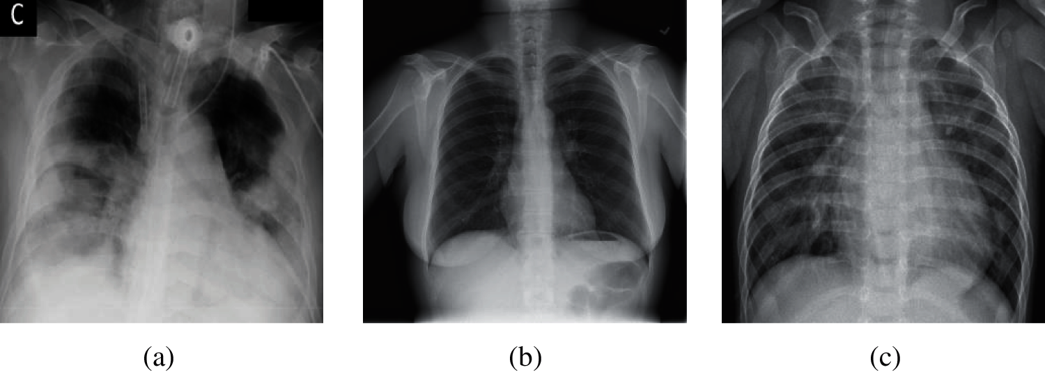
Figure 1: Samples of chest X-ray images (a) Sample of COVID-19 (b) Sample of normal (c) Sample of pneumonia
At present, scholars in mounting numbers used deep learning technology in the diagnosis COVID-19. Xu et al. [8] set the chest CT image to dataset of experiment, and used V-Net for image segmentation. Then input the segmentation results into ResNet-18 for three categories (COVID-19, Influenza and Normal) detection network. The overall accuracy of the model is 86.7%. There are some other chest CT methods reported in recent literature [9–11]. Although the chest CT images are used as the dataset in the methods mentioned above, which have low detection accuracy.
Narin et al. [12] used chest X-ray images as the dataset, and proposed three models (ResNet-50, Perception-V3, and Perception ResNet-V2) to detect COVID-19. Here, the dataset used in this experiment is divided into Normal and COVID-19, and each type image has the same numbers. The experimental results show that the ResNet-50 model has the best performance, which is 98.0%. Following by Inception V3, the accuracy is 97.0%. The last is Inception ResNet-V2, which accuracy is 87%. Although the proposed method can achieve high detection accuracy, of which structures are complex, with weak robustness and unreliable generalization of used to deal with multi-classification problems.
To solve above problems, our team proposed a novel framework and three methods to diagnose COVID-19 based on chest X-ray images. In this paper, the contributions of this study are listed as follows:
(i) A novel framework—Biogeography-based optimization Expert-VGG (BEVGG) is proposed.
(ii) Three novel methods—BEVGGC-I, BEVGGC-II, and BEVGGC-III based on the BEVGG framework are proposed.
(iii) We find our three methods are superior to state-of-the-art methods, and BEVGGC-I has the best performance of all methods.
The experimental dataset used in this paper is a public dataset from the Kaggle website [13]. This dataset consists of 6939 chest X-ray images, which are divided into three categories (COVID-19, Normal, and Pneumonia), and each category has 2313 images. The number ratio of each category of chest X-ray images is 1:1:1. In each category image, 80% of the samples were randomly selected as training set and 20% of the rest were used as test set. In Section 4, we keep the same division ratio of training set and test set to perform 10-fold cross validation. The experimental results are from NVIDIA QUADRO RTX 8000. The other parameters of the device are as follows. GPU memory is 48 GB GDDR6 with ECC. Total graphics power is 260 W. NVIDIA tensor cores is 576. NVIDIA RT cores is 72. And the total board power is 295 W. Fig. 2 shows the chest X-ray images from our dataset.
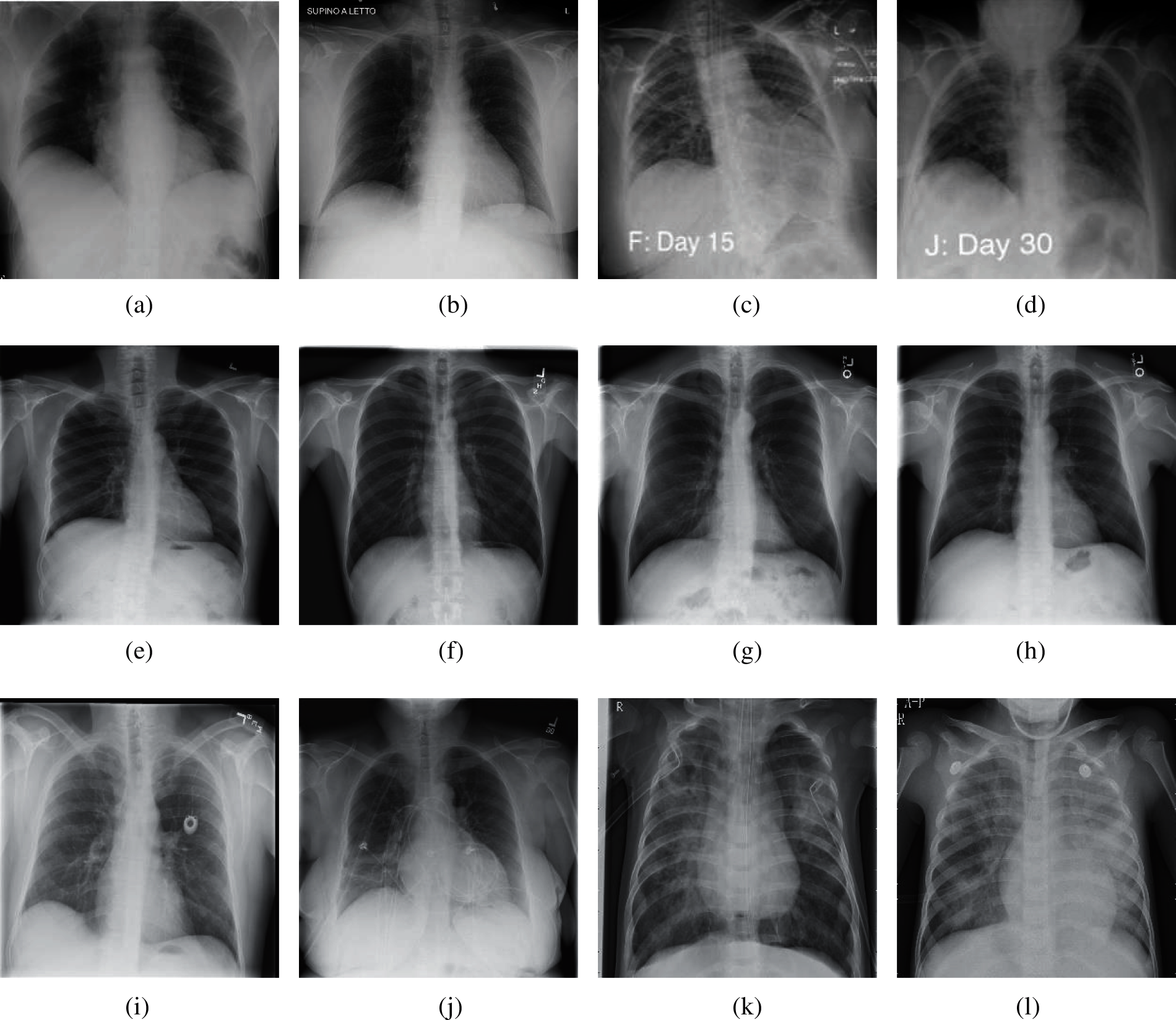
Figure 2: Samples of our dataset (a) Sample 1 of COVID-19 (b) Sample 2 of COVID-19 (c) Sample 3 of COVID-19 (d) Sample 4 of COVID-19 (e) Sample 1 of normal (f) Sample 2 of normal (g) Sample 3 of normal (h) Sample 4 of normal (i) Sample 1 of pneumonia (j) Sample 2 of pneumonia (k) Sample 3 of pneumonia (l) Sample 4 of pneumonia
According to Fig. 2, we can see that for the chest of X-ray images of COVID-19, it is usually manifested as multiple ground glass shadows and infiltrating shadows in both lungs. If the condition is serious, pulmonary consolidation can occur, but pleural effusion is rare. For the chest X-ray images of pneumonia, there are fuzzy cloud like or uniform infiltration shadow. The hilar is dense, gradually shallow outward, and the edge is not clear. It usually does not invade the whole lung lobe, most of them involve in one lung lobe, especially in the lower lobe.
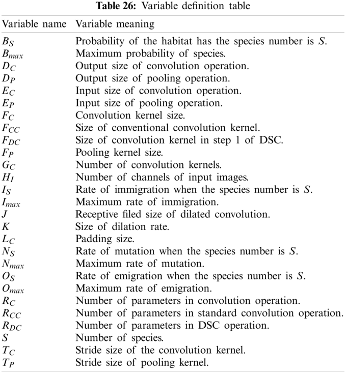
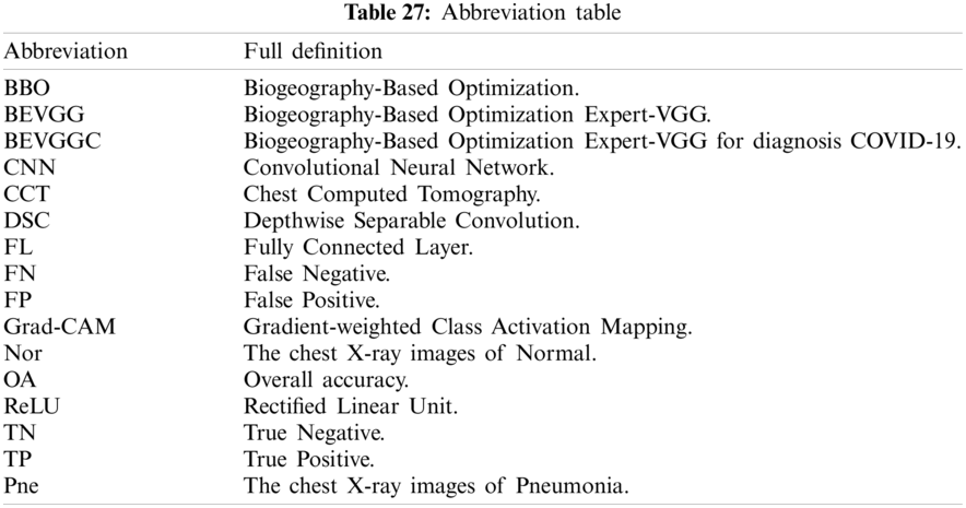
To ease the understanding of this paper, Tab. A1 shows all variables used in our study. Tab. A2 gives the abbreviation and their full names. Tabs. A1 and A2 are in the appendix at the end of the paper.
3.1 Biogeography-Based Optimization
Biogeography-based optimization (BBO) is an efficient optimization algorithm, suitable for solving high-dimensional and multi-objective optimization problems [14]. To facilitate the description of the BBO, our team introduced the following concepts: (i) Habitats. Habitats are places where species live, reproduce, mutate and die. This variable corresponds to a set of solutions in the problem to be optimized. (ii) Suitable Index Variable (SIV). This variable is used to describe the environmental variables of species living in each habitat, such as sunlight, vegetation coverage, water sources, food, etc. [15]. This variable corresponds to the independent variable in a set of solutions of the problem to be optimized [16]. (iii) Habitats Suitable Index (HSI). HSI is used to measure a habitat that is suitable for species. The value of this variable can be obtained by calculating the SIV using the objective function [17]. This variable is used to measure the suitability of a set of solutions in the problem to be optimized. Fig. 3 shows the habitats and species migration path of BBO.
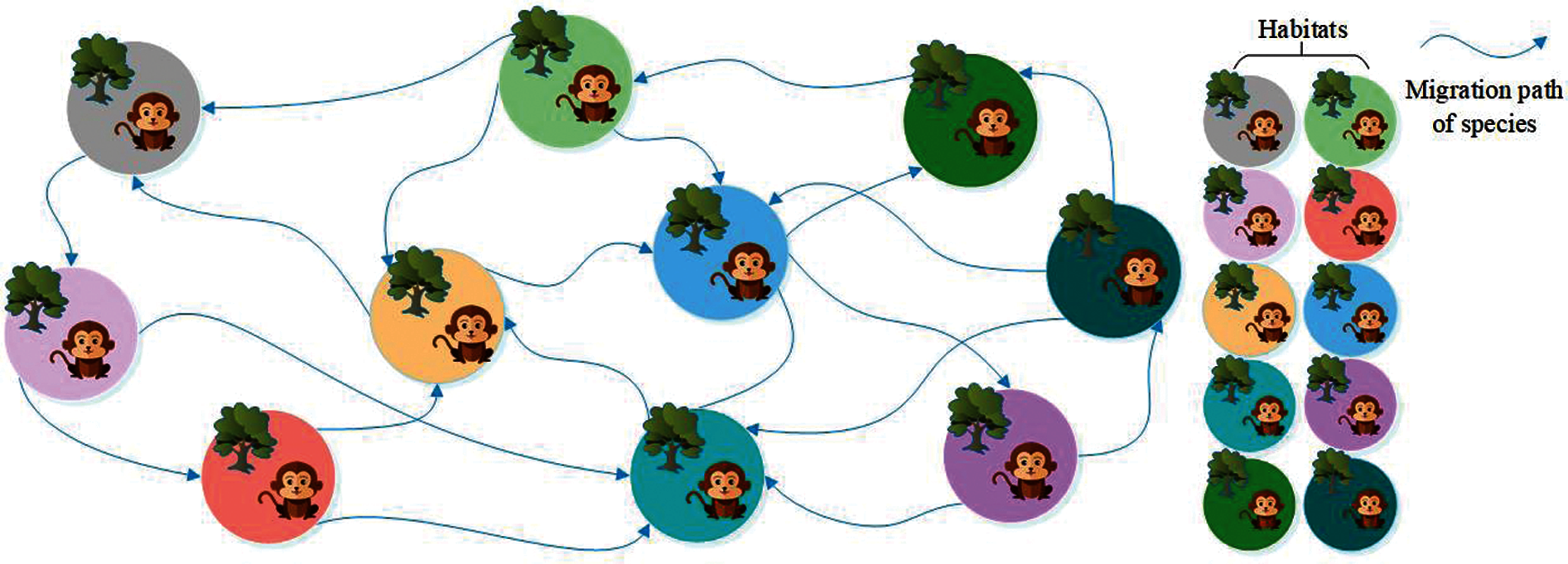
Figure 3: Habitats and species migration path of BBO
The process of BBO optimization of a problem can be divided into two stages: migration and mutation. The migration stage also can be divided into two operations: immigration and emigration. When the algorithm performs the migration operation, it determines the immigration SIV and the emigration SIV according to the migration rate [18] replaces the value of the immigration SIV with the emigration SIV. When the algorithm performs the mutation operation, it randomly generates a value for each SIV and compares it with the mutation rate. If the value is less than the mutation rate, performs mutation, viz., it randomly changes the corresponding SIV to a new value. Otherwise, the mutation is not performed. Both migration and mutation follow the following formula:
Here,
Both migration and mutation in the BBO are to improve the diversity of the solution to be optimized. The mutation is often performing after migration. At the same time, elitism is introduced to better preserve the optimal solution generated during each iteration. Through the above content, BBO has the advantages of fewer parameters, simple operation and fast convergence speed. It has a good ability to solve the problem of optimizing multiple CNN hyperparameters.
When we used BBO to optimize the hyperparameters of CNN, the corresponding relationship between BBO variables and CNN variables is as follows. SIV represents the value of the hyperparameters to be optimized. The objective function of BBO represents CNN. HSI represents the output of CNN. Habitat represents a set of solutions of all the hyperparameters to be optimized. When we perform the BBO, through continuous iteration, the optimization operation is completed.
3.2 Improvement I: A Novel Framework—BEVGG
In this section, our team proposed a novel framework for the detection COVID-19 based on chest X-ray images. Which consists of convolution layer, pooling layer and the fully connected layer.
The function of convolution operation is to extract image features on input images. The steps of convolution operation are [20]: convolution kernel calculates the image information of the receptive field with the corresponding convolution operator to obtain the image feature information [21]. The specific calculation method follows the formula (4) and (5).
Here,
Therefore, convolution operation has the characteristics of local connection and weight sharing, thus convolution operation can be used to achieve efficient and fast feature extraction of images.
The image information extracted by convolution operation can be directly fed to the fully connected layer. If this is done, the fully connected layer will handle a huge number of calculations and limit the performance of the model. Therefore, we introduced pooling operation to reduce the dimensionality of extracted features and reduce the risk of overfitting [22]. There are two common pooling operations: max-pooling and average pooling. Which are shown as Figs. 4 and 5. The following content explained them, respectively.
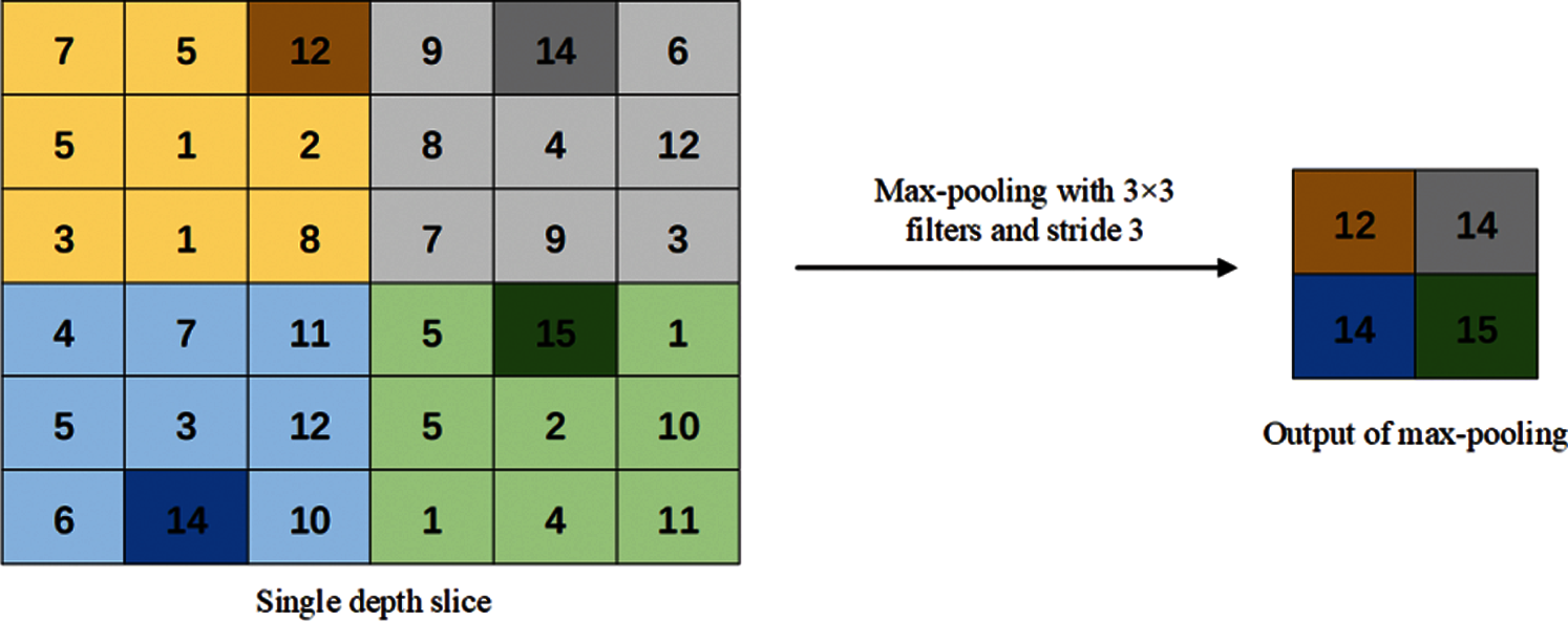
Figure 4: Max-pooling method
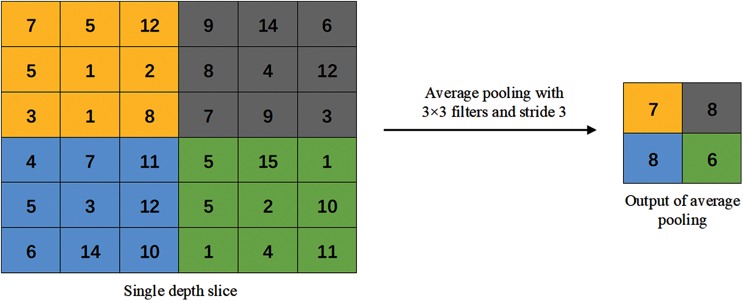
Figure 5: Average pooling method
In the max-pooling operation, the maximum value of each receptive field is selected as the output of the pooling area. Therefore, the max-pooling operation can better preserve the texture information and reduce the deviation of the estimated average value caused by convolution parameter errors.
The calculation formula of output size through pooling operation is shown as follows:
Here,
In the average pooling operation, the average of all values in each receptive field is calculated as the output of the pooling area. Therefore, the average pooling operation can better preserve the overall features of the image, highlight the background information of the image, and reduce the increase in estimation variance caused by the limited neighborhood size.
According to the above, pooling operation can both reduce the number of parameters and the risk of overfitting. It also has translation invariance.
Fig. 6 shows the framework—Biogeography-based optimization Expert-VGG (BEVGG)—our team proposed. In the feature extraction structure of BEVGG, convolution layer and pooling layer have 5 layers respectively, after each convolution layer, batch normalization and Rectified Linear Unit (ReLu) are performed. In the classification structure of BEVGG, there are three fully connected layers. For the rationality proof of the BEVGG structure, please refer to Section 4.
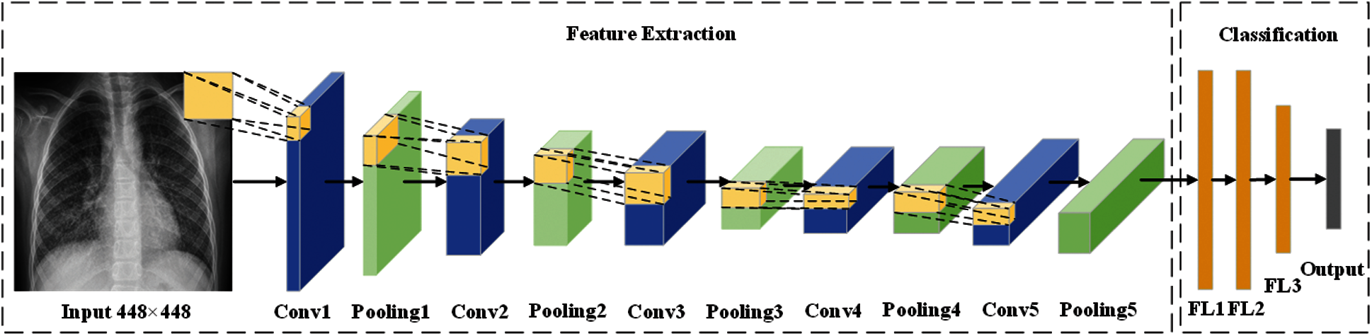
Figure 6: The structure of BEVGG
3.3 Depthwise Separable Convolution
According to the contents of Section 3.2.1, when standard convolution kernel performs convolution operation, all channels of input image in the receptive field of convolution kernel are calculated at the same time. And one convolution kernel can just extract one feature. If we want to extract more features from input images, the number of convolution kernels will be added accordingly.
Fig. 7 shows the depthwise separable convolution (DSC) that performs the convolution operation process. The biggest difference between DSC and standard convolution is that the convolution process of DSC is divided into two steps [23]. Step 1, each channel of input image is calculated by DSC kernel. Step 2, all channels of the result from step 1 are calculated at the same time by
The advantage of DSC operation is that this convolution operation can significantly reduce the number of parameters in the convolution operation.
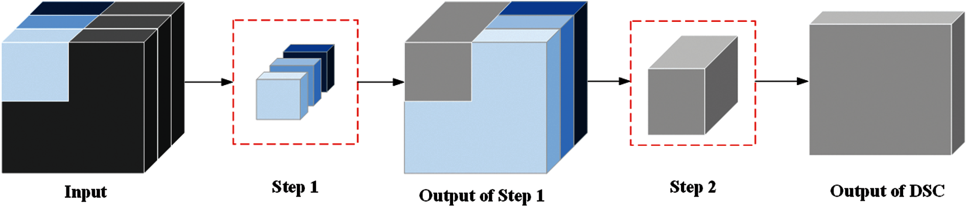
Figure 7: Convolution operation process of depthwise separable convolution
The calculated parameters methods of standard convolution and DSC are as follows:
Here,
According to the above contents, the parameters of convolution operation using DSC are less than that of using standard convolution. The more convolution kernels used in models, the parameters of convolution using DSC are less than that of using standard convolution, and the advantages of DSC are more significant.
In Section 3.2.1 and Section 3.3, we have described both the convolution operation of standard convolution and DSC. The receptive field of both of them is continuous. In this part, we introduced a convolution with discontinuous receptive field—dilated convolution [25]. The receptive field of standard convolution and dilated convolution are shown in Fig. 8. Since the receptive field of dilated convolution is filled with different numbers of blocks between each small receptive field according to different dilated rates, the dilated convolution can catch more image information than that of the convolution that has the continuous receptive field [26].
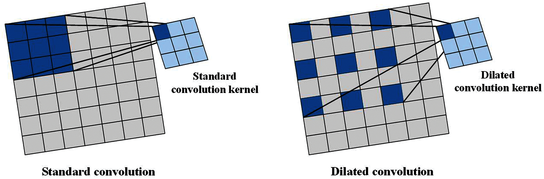
Figure 8: Two types of receptive field
The calculated method of a single dilated convolution’s receptive field is as follows:
Here,
In Section 3.5, we discussed the three methods (BEVGGC-I, BEVGGC-II, and BEVGGC-III) proposed by our team based.
3.5 Improvement II: Three Methods—BEVGGC-I, BEVGGC-II, and BEVGGC-III
In this section, we described three methods proposed by our team (BEVGGC-I, BEVGGC-II, and BEVGGC-III). The structures of them are shown as Figs. 9–11. Here, we also used BBO to optimize the values of different hyperparameters of our methods as shown in Fig. 9.
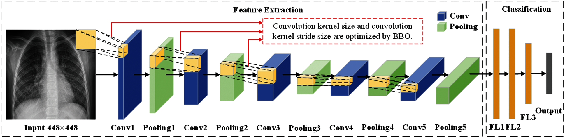
Figure 9: The structure of BEVGGC-I
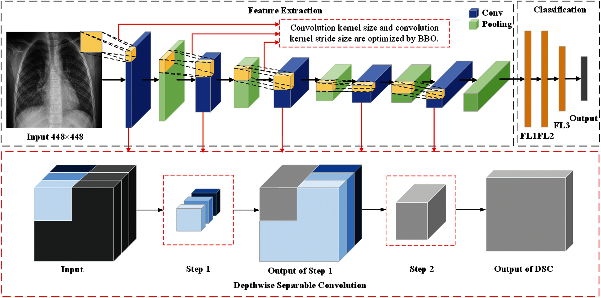
Figure 10: The structure of BEVGGC-II
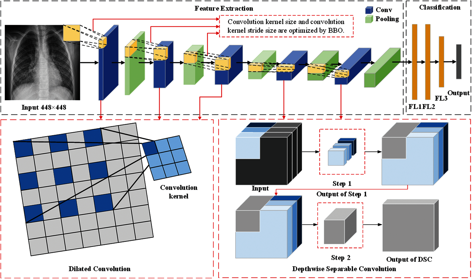
Figure 11: The structure of BEVGGC-III
In the structure of BEVGGC-I, we set all the convolutional layers to standard convolutional layers. And we used BBO to optimize the standard convolution kernel size and stride size of the first three convolutional layers. The other parameters (weights, biases) of the model are optimized by back propagation simultaneously. BEVGG has five convolution layers. Due to experimental conditions, we choose the hyperparameters in the first three convolution layers for optimization.
In the process of BBO optimizing the BEVGGC-I hyperparameters, each convolution kernel size and convolution kernel stride size in the first three convolutional layers as each SIV. By continuously changing the candidate values of each SIV, the array of all SIVs is as a habitat. And the value of the CNN output is as HSI of each habitat. Through continuous performance of iterative operations, the output after BBO optimized is obtained. The following BBO optimizes hyperparameters of models refer to this method.
In the structure of BEVGGC-II, we set all the convolutional layers to depthwise separable convolutional layers. And we used BBO to optimize the depthwise separable convolution kernel size and stride size of the first three convolutional layers. The other parameters (weights, biases) of the model are optimized by back propagation simultaneously.
In the structure of BEVGGC-III, we set the first three convolutional layers are dilated convolutional layers, the remaining convolutional layers are depthwise separable convolutional layers. Here, to make the model shows better performance, we determined the dilated rate value is 2 through trial and error. And we also used BBO to optimize the dilated convolution kernel size and stride size of the first three convolutional layers. The other parameters (weights, biases) of the model are optimized by back propagation simultaneously.
To compare the diagnostic performance of different methods, confusion matrix [28] is introduced as shown in Tab. 1. Here, TP represents the predicted class and the actual class both are positive. TN represents the predicted class and the actual class both are negative. FP represents the predicted class is positive, but the actual class is negative. And FN represents the predicted class is negative, but the actual class is positive [29].
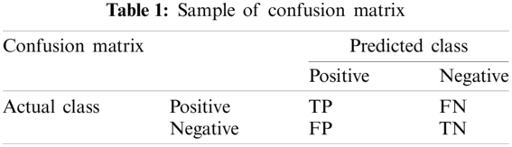
Besides, we defined five metrics: Accuracy, Precision, Sensitivity, Specificity and F1 scores.
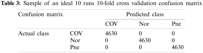
To prove the robustness of the methods, 10 runs 10-fold cross validation is introduced. Therefore, we divided the experimental dataset randomly according to the dividing method of 10-fold cross validation, and obtained 10 same size new datasets with different data distribution based on the original experimental dataset. In the selection of test set, we select two increasing number subsets as test set, and the remaining 8 subsets as training set. And our experiments are carried out on these datasets.
According to the above contents, an ideal confusion matrix of our experiment is as Tab. 2.
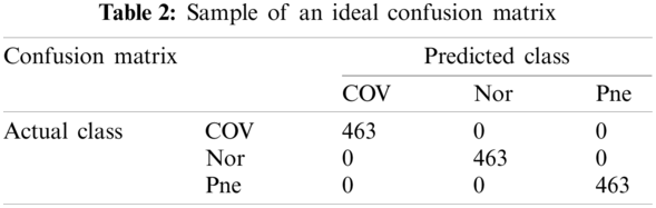
An ideal 10 runs 10-fold cross validation confusion matrix is shown as Tab. 3. According to the selection method of test set, the number of each category in Tab. 2 is 463 and the number of each category in Tab. 3 is 4630.
To better understand the performance of different methods, Gradient-weighted Class Activation Mapping (Grad-CAM) is introduced. By analyzing the Grad-CAM result of original chest X-ray images of each method, we can more intuitively compare the detection performance between different methods. Fig. 12 shows the Grad-CAM result image of an original chest X-ray images. It is worth noting that the higher color brightness areas in Grad-CAM result image, the greater the output reference weight.
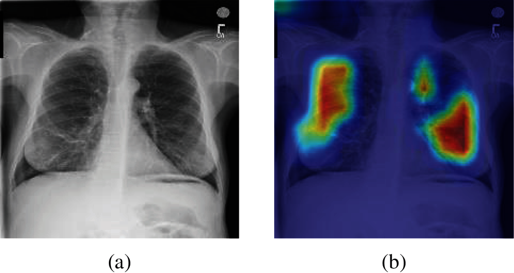
Figure 12: A sample of Grad-CAM result of the original chest X-ray images (a) A sample of the original Chest X-ray images (b) Grad-CAM result of (a)
4 Experiment Results and Discussions
In this part, we have compared, analyzed and discussed the experimental results. Besides, we also compared our methods with state-of-the-art methods.
4.1 Ablation Experiments of BEVGGC
In this section, ablation experimental results of BEVGGC are shown to prove the rationality of the structure proposed by our team of BEVGGC (13 layers of the feature extraction structure and 3 layers of the fully connected layer).
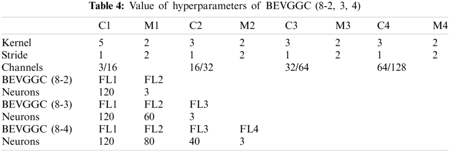
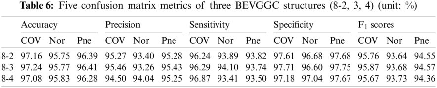
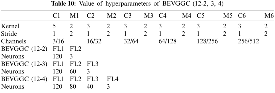
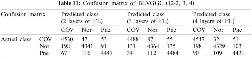
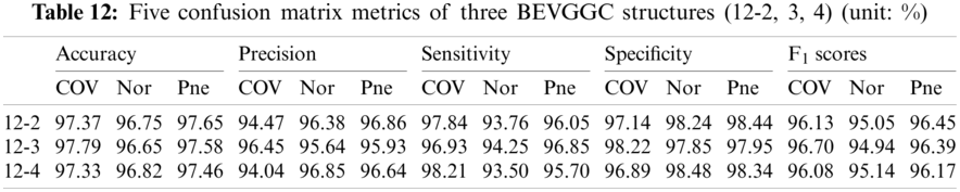
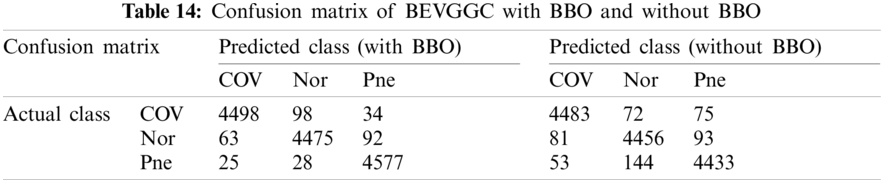
Tabs. 5, 8 and 11 show the confusion matrix of BEVGGC with 9 different structures. Tabs. 6, 9 and 12 show the four confusion matrix metrics corresponding to the above confusion matrix, respectively. And Tabs. 14 and 15 show the results of BEVGGC optimized by BBO. Here, FL represents the fully connected layer. COV represents the chest X-ray images of COVID-19. Nor represents the chest X-ray images of Normal. And Pne represents the chest X-ray images of Pneumonia. BEVGGC (8-2) represents the BEVGGC with 8 layers of feature extraction structure and 2 layers of the fully connected layer. BEVGGC (8-3) represents the BEVGGC with 8 layers of feature extraction structure and 3 layers of the fully connected layer. BEVGGC (8-4) represents the BEVGGC with 8 layers of feature extraction structure and 4 layers of the fully connected layer. For other similar descriptions, please refer to the above content.
In Tabs. 4, 7 and 10, the C1 represents the first convolutional layer of BEVGGC. M1 represents the first max-pooling layer of BEVGGC. FL1 represents the first fully connected layer of BEVGGC. Other similar descriptions refer to this content. And the following contents refer to this definition.
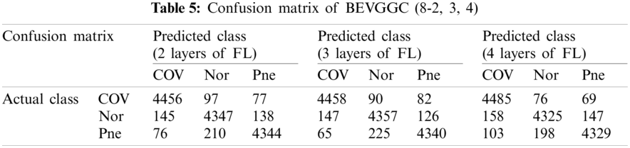
As can be seen from Tab. 6, all three have the highest accuracy for COV, followed by Pne, the lowest accuracy for Nor. BEVGGC (8-2) and BEVGGC (8-4) have the highest precision for Pne. BEVGGC (8-3) has the highest precision for COV. All three have the highest sensitivity to COV, the highest specificity to Pne and the highest F1 scores to COV.
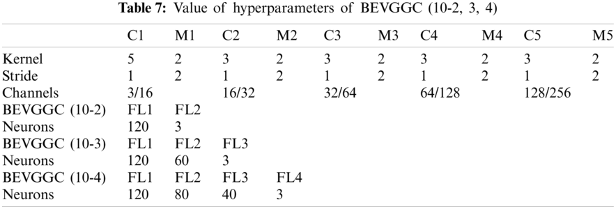
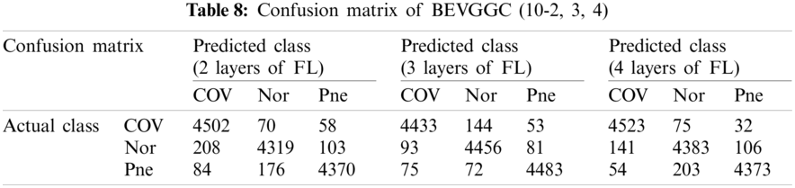
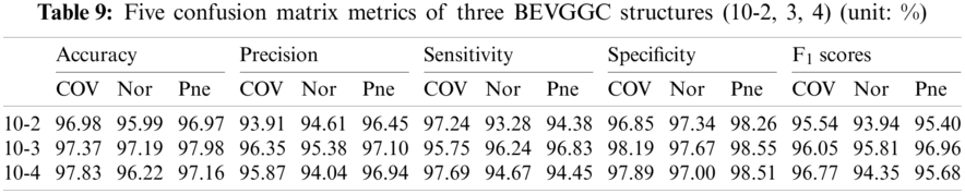
As can be seen from Tab. 9, BEVGGC (10-2) and BEVGGC (10-4) have the highest accuracy for COV. BEVGGC (10-3) has the highest accuracy for Pne. All three have the highest precision for Pne. BEVGGC (10-2) and BEVGGC (10-4) have the highest sensitivity for COV. BEVGGC (10-3) has the highest sensitivity to Pne. And all three have the highest specificity to Pne. BEVGGC-I and BEVGGC-III have the highest F1 score to COV, BEVGGC-II has the highest F1 score to Pne. Here, the data of BEVGGC (10-3) in Tabs. 8 and 9 are the data of BEVGGC-I.
As can be seen from Tab. 12, BEVGGC (12-2) and BEVGGC (12-4) have the highest accuracy for Pne. BEVGGC (12-3) has the highest accuracy for COV. BEVGGC (12-2) has the highest precision for Pne. BEVGGC (12-3) has the highest precision for COV. BEVGGC (12-4) has the highest precision for Nor. All three have the highest sensitivity to COV. BEVGGC (12-2) has the highest specificity for Pne. BEVGGC (12-3) has the highest specificity for COV. And BEVGGC (12-4) has the highest specificity for Nor. BEVGGC-I and BEVGGC-III have the highest F1 score to Pne. BEVGGC-II has the highest F1 score to COV. From the above contents, it can be seen that the model performance of BEVGGC (10-3) is the best. Therefore, we define BEVGGC represents the structure of BEVGGC (10-3) in the following content.
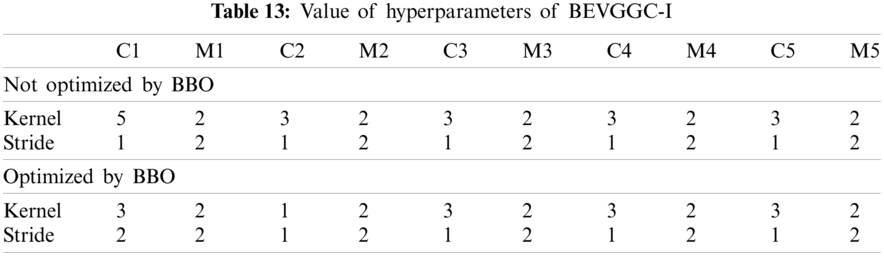
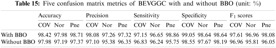
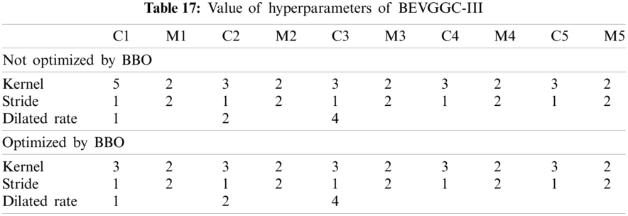
As can be seen from Tab. 13, the value of hyperparameters in the C1 and C2 are changed when BEVGGC-I optimized by BBO. As can be seen from Tab. 15, the BEVGGC with BBO has the highest accuracy for Pne. The BEVGGC without BBO has the highest accuracy for COV. Both methods have the highest precision for COV. BEVGGC with BBO has the highest sensitivity to Pne and BEVGGC without BBO has the highest sensitivity to COV. Besides, two methods have the highest specificity for COV. BEVGGC with BBO has the highest F1 score to Pne. BEVGGC without BBO has the highest F1 score to COV. Therefore, Tab. 15 shows the effectiveness of BBO to optimize the values of hyperparameters of CNN. Therefore, we define BEVGGC-I represents BEVGGC-I (with BBO), BEVGGC-II represents the BEVGGC-II (with BBO), and BEVGGC-III represents BEVGGC-III (with BBO) in the following content. Tab. 16 shows the value of hyperparameters of BEVGGC-II. Tab. 17 shows the value of hyperparameters of BEVGGC-III. And Tab. 18 shows the confusion matrix of BEVGGC-II and BEVGGC-III.

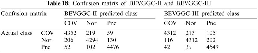
As seen from Tab. 19, both methods have the highest accuracy for Pne. BEVGGC-II has the highest precision for Pne. BEVGGC-III has the highest precision for COV. Both of them have the highest sensitivity to Pne. BEVGGC-II has the highest specificity for Pne. And BEVGGC-III has the highest specificity for COV. Both of them have the highest F1 score to Pne.
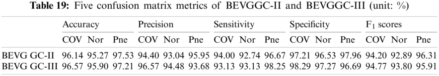
It can be seen from Tab. 15 that the accuracy of BEVGGC-I for COV is 98.42%, 2.28% higher than that of BEVGGC-II, and 1.85% higher than that of BEVGGC-III. The accuracy of BEVGGC-I for Nor is 97.98%, 2.17% higher than that of BEVGGC-II, and 2.08% higher than that of BEVGGC-III. The accuracy of BEVGGC-I for Pne is 98.71%, 1.18% higher than that of BEVGGC-II, and 1.5% higher than that of BEVGGC-III. The precision for COV of BEVGGC-I is 98.08%, which is 3.68% higher than that of BEVGGC-II and 1.51% higher than that of BEVGGC-III. The sensitivity to COV of BEVGGC-I is 97.15%, which is 3.15% higher than that of BEVGGC-II and 4.02% higher than that of BEVGGC-III. The specificity for COV of BEVGGC-I is 99.05%, which is 1.84% higher than that of BEVGGC-II and 0.76% higher than that of BEVGGC-III. Therefore, BEVGGC-I has the best detection performance in accuracy, precision, sensitivity and specificity of all methods.
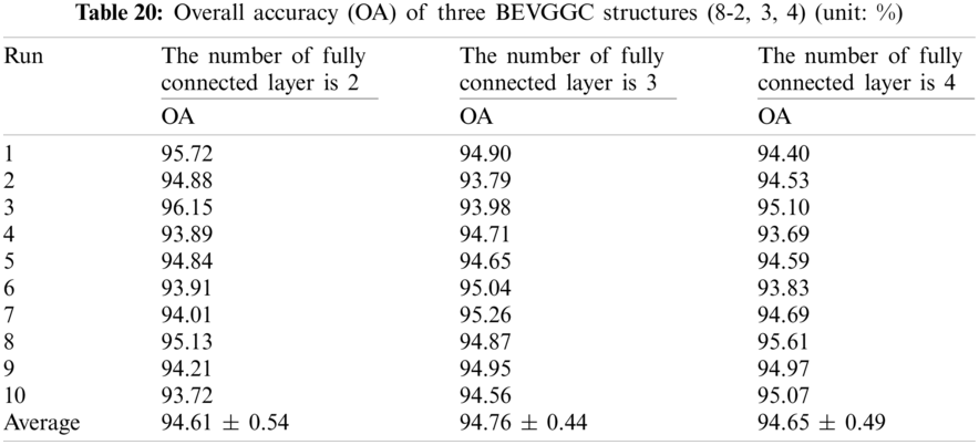
It can be seen from Tab. 20 that the OA of BEVGGC (8-2) is 0.15% ± 0.1% lower than that of BEVGGC (8-3), and BEVGGC (8-4) is 0.11% ± 0.05% lower than that of BEVGGC (8-3). Which shows that the 8 layers of the feature extract structure and 3 fully connected layers of BEVGGC have the best performance is 94.76% ± 0.44%.
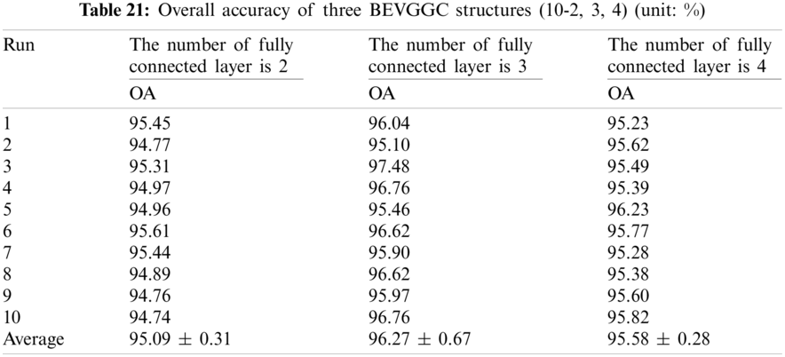
It can be seen from Tab. 21 that the OA of BEVGGC (10-2) is 1.18% ± 0.36% lower than that of BEVGGC (10-3), and BEVGGC (10-4) is 0.69% ± 0.39% lower than that of BEVGGC (10-3). Which shows that the 10 layers of the feature extract structure and 3 fully connected layers of BEVGGC have the best performance is 96.27% ± 0.67%.
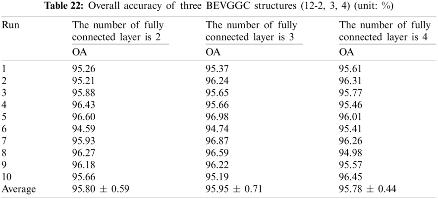
It can be seen from Tab. 22 that the OA of BEVGGC (12-2) is 0.15% ± 0.12% lower than that of BEVGGC (12-3), and BEVGGC (12-4) is 0.17% ± 0.27% lower than that of BEVGGC (12-3). Which shows that the 12 layers of the feature extract structure and 3 fully connected layers of BEVGGC have the best performance is 95.95% ± 0.71%.
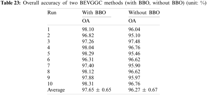
It can be seen from Tab. 23 that the OA of BEVGGC with BBO is 1.38% ± 0.02% higher than that of BEVGGC without BBO. Which shows that BBO can optimize the hyperparameters of convolutional neural network. In conclusion, BEVGGC (with BBO) has the best detection performance to diagnose COVID-19 based on chest X-ray images.
In this section we listed the OA of three methods (BEVGGC-I, BEVGGC-II, and BEVGGC-III). Detailed data is shown in Tab. 24.
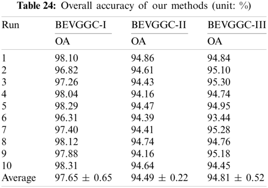
It can be seen from Tab. 24, BEVGGC-I has the highest OA, which is 97.65% ± 0.65%. The OA of BEVGGC-I is 3.16% ± 0.43% higher than that of BEVGGC-II, 2.84% ± 0.13% higher than that of BEVGGC-III. Our team believes that the reasons for this result are: (i) all convolutional layers of BEVGGC-II are depthwise separable convolutional layers. According to the property of depthwise separable convolution, we can see that BEVGGC-II has fewer parameters than BEVGGC-I, but it reduces OA. (ii) depthwise separable convolution and dilated convolution are both used in BEVGGC-III. Since the first three convolutional layers of BEVGGC-III are dilated convolutional layer. Based on setting the rational dilated rate of dilated convolution, the receptive field of convolution kernels can be expanded and the advantages of dilated convolution can be fully displayed. Besides, the remaining convolutional layers of BEVGGC-III are depthwise separable convolutional layers. Therefore, BEVGGC-III has higher OA than BEVGGC-II and lower OA than BEVGGC-I. In conclusion, using the standard convolutional layer methods—BEVGGC-I has the best diagnosis performance. And this is consistent with the conclusion in Section 4.1, which proves the reliability and efficiency of BEVGGC-I.
In this section, we analyzed the Grad-CAM result of our methods, which can help us understand the performance of different methods more intuitively.
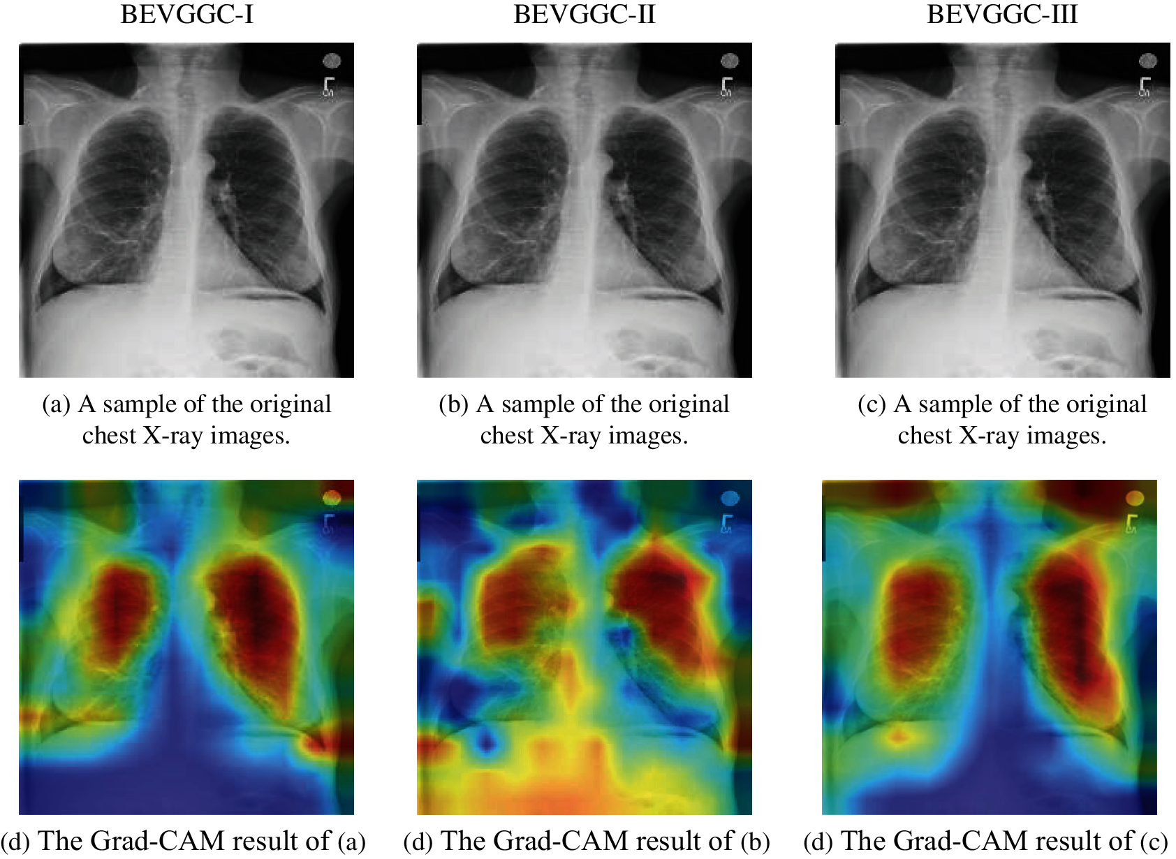
Figure 13: Grad-CAM results of our methods. (a) A sample of the original chest X-ray images. (b) A sample of the original chest X-ray images. (c) A sample of the original chest X-ray images. (d) The Grad-CAM result of (a). (e) The Grad-CAM result of (b). (f) The Grad-CAM result of (c)
Fig. 13 shows the Grad-CAM results of our methods. The high brightness color areas in the Gram-CAM result of BEVGGC-I are concentrated on the chest. The high brightness color areas in the Gram-CAM result of BEVGGC-II are most concentrated on the chest, but some of them are also in the abdomen. And the high brightness color area in the Gram-CAM result of BEVGGC-III are almost concentrated on the chest, and some of them are distributed outside the human body. Therefore, the Grad-CAM results are consistent with the OA ranking of our methods.
4.4 Comparison to State-of-the-Art Approaches
In this section, we compared our three methods with two state-of-the-art methods (VGG-16 [30], ResNet-18 [31]). Tab. 25 lists the comparison result of all methods.
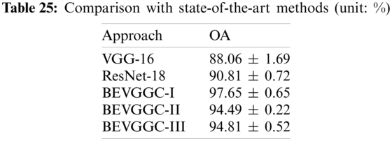
As can be seen from Tab. 25, compared with the state-of-the-art methods, the OA of BEVGGC-I is 9.59% ± 1.04% higher than that of VGG-16, 6.84% ± 0.07% higher than that of ResNet-18. The OA of BEVGGC-II is 6.43% ± 1.47% higher than that of VGG-16, 3.68% ± 0.5% higher than that of ResNet-18. The OA of BEVGGC-III is 6.75% ± 1.17% higher than that of VGG-16, 4.0% ± 0.2% higher than that of ResNet-18. And the OA of BEVGGC-I is 3.16% ± 0.43% higher than that of BEVGGC-II, 2.84% ± 0.13% higher than that of BEVGGC-III. Therefore, BEVGGC-I has the best performance and the validity of our study is verified by Tab. 25.
In this paper, we proposed three methods (BEVGGC-I, BEVGGC-II, and BEVGGC-III) to diagnose COVID-19 based on chest X-ray images and used BBO to optimize the values of hyperparameters of the methods. Among them, BEVGGC-I (97.65% ± 0.65%) has the best detection performance, followed by BEVGGC-III (94.81% ± 0.52%), and the last is BEVGGC-II (94.49% ± 0.22%). The experimental result shows that all of our methods are superior to the state-of-the-art methods in the OA of model.
In the next study, we will continue to work on the artificial intelligence medical image aided diagnosis system by using deep learning technology. Our main research directions are: (i) we will try to use more optimization methods [32–35] to optimize the values of hyperparameters of CNN. (ii) we will propose a more rationally convolutional neural network to diagnose the medical images.
Funding Statement: Key Science and Technology Program of Henan Province, China (212102310084), J. Sun, X. Li, and C. Tang received the grant. Provincial Key Laboratory for Computer Information Processing Technology, Soochow University (KJS2048), J. Sun received the grant.
Conflicts of Interest:The authors declare that they have no conflicts of interest to report regarding the present study.
1. Wang, S. H., Nayak, D. R., Guttery, D. S., Zhang, X., Zhang, Y. D. (2021). COVID-19 classification by CCSHNet with deep fusion using transfer learning and discriminant correlation analysis. Information Fusion, 68, 131–148. DOI 10.1016/j.inffus.2020.11.005. [Google Scholar] [CrossRef]
2. Zhang, Y. D., Satapathy, S. C., Zhang, X., Wang, S. H. (2021). COVID-19 diagnosis via densenet and optimization of transfer learning setting. Cognitive Computation, (5), 1–17. DOI 10.1007/s12559-020-09776-8. [Google Scholar] [CrossRef]
3. Dara, N., Sharifi, N., Boroujeni, M. G., Hosseini, A., Sayyari, A. (2021). COVID-19 pneumonia in a child with hepatic encephalopathy: A case study. Iranian Journal of Child Neurology, 15(1), 113–118. DOI 10.22037/ijcn.v15i1.30879. [Google Scholar] [CrossRef]
4. Tabatabaeizadeh, S. A. (2021). Airborne transmission of COVID-19 and the role of face mask to prevent it: A systematic review and meta-analysis. European Journal of Medical Research, 26(1). 1–6. DOI 10.1186/s40001-020-00475-6. [Google Scholar] [CrossRef]
5. Pham, T. D. (2020). Classification of COVID-19 chest x-rays with deep learning: New models or fine tuning? Health Information Science and Systems, 9(1), 1–11. DOI 10.1007/s13755-020-00135-3. [Google Scholar] [CrossRef]
6. Bayramoglu, Z., Canıpek, E., Cömert, R. G., Gasimli, N., Kaba, Ö. et al. (2020). Imaging features of pediatric COVID-19 on chest radiography and chest CT: A retrospective, single-center study. Academic Radiology, 28(1), 18–27. DOI 10.1016/j.acra.2020.10.002. [Google Scholar] [CrossRef]
7. Chandra, T. B., Verma, K., Singh, B. K., Jain, D., Netam, S. S. (2020). Coronavirus disease (COVID-19) detection in chest X-ray images using majority voting based classifier ensemble. Expert Systems with Applications, 165(2), 113909. DOI 10.1016/j.eswa.2020.113909. [Google Scholar] [CrossRef]
8. Xu, X., Jiang, X., Ma, C., Du, P., Li, X. et al. (2020). A deep learning system to screen novel coronavirus disease 2019 pneumonia. Engineering, 6(10), 1122–1129. DOI 10.1016/j.eng.2020.04.010. [Google Scholar] [CrossRef]
9. Wang, S. H., Wu, X., Zhang, Y. D., Tang, C., Zhang, X. (2020). Diagnosis of COVID-19 by wavelet renyi entropy and three-segment biogeography-based optimization. International Journal of Computational Intelligence Systems, 13(1), 1332–1344. DOI 10.2991/ijcis.d.200828.001. [Google Scholar] [CrossRef]
10. Wang, S. H., Govindaraj, V., Gorriz, J. M., Zhang, X., Zhang, Y. D. (2020). COVID-19 classification by FGCNet with deep feature fusion from graph convolutional network and convolutional neural network. Information Fusion, 67, 208–229. DOI 10.1016/j.inffus.2020.10.004. [Google Scholar] [CrossRef]
11. Zhang, Y. D., Satapathy, S. C., Liu, S., Li, G. R. (2021). A five-layer deep convolutional neural network with stochastic pooling for chest CT-based COVID-19 diagnosis. Machine Vision and Applications, 32(1), 1–13. DOI 10.1007/s00138-020-01119-9. [Google Scholar] [CrossRef]
12. Narin, A., Kaya, C., Pamuk, Z. (2021). Automatic detection of coronavirus disease (COVID-19) using X-ray images and deep convolutional neural networks. Pattern Analysis and Applications, 6, 1–14. DOI 10.1007/s10044-021-00984-y. [Google Scholar] [CrossRef]
13. Asraf, A. (2020). COVID19 with pneumonia and normal chest xray(PA) datase. https://www.kaggle.com/amanullahasraf/covid19-pneumonia-normal-chest-xray-pa-dataset. [Google Scholar]
14. Ghobaei-Arani, M. (2021). A workload clustering based resource provisioning mechanism using biogeography based optimization technique in the cloud based systems. Soft Computing, 25(4), 1–18. DOI 10.1007/s00500-020-05409-2. [Google Scholar] [CrossRef]
15. Dwivedi, A. K., Sharma, A. K. (2020). I-FBECS: Improved fuzzy based energy efficient clustering using biogeography based optimization in wireless sensor network. Transactions on Emerging Telecommunications Technologies, 32(2), e4205. DOI 10.1002/ett.4205. [Google Scholar] [CrossRef]
16. Ghatte, H. F. (2021). A hybrid of firefly and biogeography-based optimization algorithms for optimal design of steel frames. Arabian Journal for Science and Engineering, 46(1), 4703–4717. DOI 10.1007/s13369-020-05118-w. [Google Scholar] [CrossRef]
17. Alam, S. J., Arya, S. R., Jana, R. K. (2020). Biogeography based optimization strategy for UPQC PI tuning on full order adaptive observer based control. IET Generation, Transmission & Distribution, 15(2), 279–293. DOI 10.1049/gtd2.12020. [Google Scholar] [CrossRef]
18. Tamilarasan, N., Lenin, S. B., Jayapandian, N., Subramanian, P. (2021). Hybrid shuffled frog leaping and improved biogeography-based optimization algorithm for energy stability and network lifetime maximization in wireless sensor networks. International Journal of Communication Systems, 34(2), e4722. DOI 10.1002/dac.4722. [Google Scholar] [CrossRef]
19. Abuelrub, A., Khamees, M., Ababneh, J., Al-Masri, H. (2020). Hybrid energy system design using greedy particle swarm and biogeography-based optimisation. IET Renewable Power Generation, 14(10), 1657–1667. DOI 10.1049/iet-rpg.2019.0858. [Google Scholar] [CrossRef]
20. Shakya, A., Biswas, M., Pal, M. (2021). Parametric study of convolutional neural network based remote sensing image classification. International Journal of Remote Sensing, 42(7), 2663–2685. DOI 10.1080/01431161.2020.1857877. [Google Scholar] [CrossRef]
21. Zhang, Y. D., Satapathy, S., Guttery, D. S., Gorriz, J. M., Wang, S. H. (2021). Improved breast cancer classification through combining graph convolutional network and convolutional neural network. Information Processing and Management, 58(2), 102439. DOI 10.1016/j.ipm.2020.102439. [Google Scholar] [CrossRef]
22. Sahani, M., Dash, P. K. (2021). FPGA-based deep convolutional neural network of process adaptive VMD data with online sequential RVFLN for power quality events recognition. IEEE Transactions on Power Electronics, 36(4), 4006–4015. DOI 10.1109/TPEL.2020.3023770. [Google Scholar] [CrossRef]
23. Le, D. N., Parvathy, V. S., Gupta, D., Khanna, A., Rodrigues, J. et al. (2021). IoT enabled depthwise separable convolution neural network with deep support vector machine for COVID-19 diagnosis and classification. International Journal of Machine Learning and Cybernetics, 1, 1–14. DOI 10.1007/s13042-020-01248-7. [Google Scholar] [CrossRef]
24. Vorugunti, C. S., Pulabaigari, V., Mukherjee, P., Sharma, A. (2020). DeepfuseOSV: Online signature verification using hybrid feature fusion and depthwise separable convolution neural network architecture. IET Biometrics, 9(6), 259–268. DOI 10.1049/iet-bmt.2020.0032. [Google Scholar] [CrossRef]
25. Kim, S., Park, I., Kwon, S., Han, J. (2020). Motion retargetting based on dilated convolutions and skeleton-specific loss functions. Computer Graphics Forum, 39(2), 497–507. DOI 10.1111/cgf.13947. [Google Scholar] [CrossRef]
26. Zhang, Y. D., Dong, Z., Wang, S. H., Yu, X., Yao, X. et al. (2020). Advances in multimodal data fusion in neuroimaging: Overview, challenges, and novel orientation. Information Fusion, 64, 149–187. DOI 10.1016/j.inffus.2020.07.006. [Google Scholar] [CrossRef]
27. Schuster, R., Wasenmuller, O., Unger, C., Stricker, D. (2019). SDC—Stacked dilated convolution: A unified descriptor network for dense matching tasks. 2019 IEEE/CVF Conference on Computer Vision and Pattern Recognition, pp. 2551–2560. Long Beach, CA. [Google Scholar]
28. Chicco, D., Totsch, N., Jurman, G. (2021). The Matthews correlation coefficient (MCC) is more reliable than balanced accuracy, bookmaker informedness, and markedness in two-class confusion matrix evaluation. BioData Mining, 14(1), 13. DOI 10.1186/s13040-021-00244-z. [Google Scholar] [CrossRef]
29. Radoux, J., Bogaert, P. (2020). About the pitfall of erroneous validation data in the estimation of confusion matrices. Remote Sensing, 12(24), 4128. DOI 10.3390/rs12244128. [Google Scholar] [CrossRef]
30. Shah, U., Abd-Alrazeq, A., Alam, T., Househ, M., Shah, Z. (2020). An efficient method to predict pneumonia from chest x-rays using deep learning approach. Studies in Health Technology and Informatics. The Importance of Health Informatics in Public Health During a Pandemic, vol. 272, pp. 457–460. Amsterdam: IOS Press. [Google Scholar]
31. Rahman, T., Chowdhury, M. E. H., Khandakar, A., Islam, K. R., Islam, K. F. et al. (2020). Transfer learning with deep convolutional neural network (CNN) for pneumonia detection using chest X-ray. Applied Sciences, 10(9), 3233. DOI 10.3390/app10093233. [Google Scholar] [CrossRef]
32. Lalwani, S., Sharma, H., Satapathy, S. C., Deep, K., Bansal, J. C. (2019). A survey on parallel particle swarm optimization algorithms. Arabian Journal for Science and Engineering, 44(4), 2899–2923. DOI 10.1007/s13369-018-03713-6. [Google Scholar] [CrossRef]
33. Rajinikanth, V., Satapathy, S. C., Dey, N., Fernandes, S. L., Manic, K. S. (2019). Skin melanoma assessment using kapur’s entropy and level set—A study with bat algorithm. Smart Intelligent Computing and Applications, vol. 104, pp. 193–202. Singapore: Springer. DOI 10.1007/978-981-13-1921-1_19. [Google Scholar] [CrossRef]
34. Satapathy, S., Naik, A. (2016). Social group optimization (SGOA new population evolutionary optimization technique. Complex & Intelligent Systems, 2(3), 173–203. DOI 10.1007/s40747-016-0022-8. [Google Scholar] [CrossRef]
35. Katari, V., Satapathy, S. C., Murthy, J., Reddy, P. (2007). Hybridized improved genetic algorithm with variable length chromosome for image clustering abstract. International Journal of Computer Science & Network Security, 7(11), 121–131. [Google Scholar]
 | This work is licensed under a Creative Commons Attribution 4.0 International License, which permits unrestricted use, distribution, and reproduction in any medium, provided the original work is properly cited. |