Computer Modeling in Engineering & Sciences

DOI: 10.32604/cmes.2021.016766

ARTICLE

A Simplified Approach of Open Boundary Conditions for the Smoothed Particle Hydrodynamics Method

Thanh Tien Bui1,*, Yoshihisa Fujita2 and Susumu Nakata2

1Graduate School of Information Science and Engineering, Ritsumeikan University, Shiga, 525-8577, Japan
2College of Information Science and Engineering, Ritsumeikan University, Shiga, 525-8577, Japan
*Corresponding Author: Thanh Tien Bui. Email: gr0399rr@ed.ritsumei.ac.jp
Received: 24 March 2021; Accepted: 12 July 2021

1  Introduction

Open boundary conditions pose an interesting challenge that has attracted a number of investigations by different authors. The simplest and fastest technique, periodic boundary conditions [1,2], is often used in which particles are recycled with the particles passing through the outlet and being re-inserted at the inlet. This technique is limited and is inappropriate for simulations with different inflow/outflow cross-sectional lengths. In addition, violations resulting from the outlet velocity field after re-insertion can cause an unstable state in long runtime simulations. Lastiwka et al. [3] proposed permeable boundary conditions; however, this is difficult to implement with a free surface. A different approach relies on a generalization of the unified semi-analytical boundary condition method introduced by Ferrand et al. [4] and Leroy et al. [5]. This technique has been used to impose unsteady open boundaries in incompressible SPH and weakly compressible SPH models. Tafuni et al. [6] used mirrored particles at the fluid zone and a higher-order interpolation process to update the values of the inflow/outflow particles. However, these approaches have a high computational cost and are complicated. Federico et al. [7] presented an implementation of open boundary conditions based on inflow/outflow buffer layers with the inflow particle information assigned at the beginning of the simulation. Alvarado-Rodrıguez et al. [8] utilized a reservoir buffer to prevent a reflection of the velocity field at the outlet. Vacondio et al. [9] introduced open boundary conditions using Riemann invariants. Tarksalooyeh et al. [10] constructed a pre-inlet domain to feed the inflow region. Molteni et al. [11] and Altomare et al. [12] proposed a sponge layer to avoid spurious reflections from waves. Liu et al. [13] used a Taylor series expansion to extrapolate the values of the inlet and outlet particles. Wang et al. [14] and Negi et al. [15] selected a characteristic-based method to apply as a non-reflecting boundary condition in a weakly compressible SPH model. Most previous studies have usually opted to update the inflow/outflow particle information via an extrapolation from the fluid particles. This results in troublesome procedures and is time consuming.

The rapid development of variants of the SPH model, specifically the δ+-SPH scheme [16], has provided reliable results, stability, and high accuracy for a variety of numerical simulations. In the δ+-SPH scheme, density variations were preserved lower than 1% while tensile instability is prevented by applying the particle shifting technique (PST). These advantages of this scheme are used to develop a simplified approach of open boundary conditions in this paper.

To simplify the treatment of the open boundary condition, in the present study, we propose a fast and simple approach based on the δ+-SPH scheme. Instead of implementing a renormalization process using the fluid particles to update the inflow/outflow particle information, we simply treat these particles as the same fluid particles or impose prescribed values to ensure the appropriate evolution of the flow field. This scheme can handle the generation of new inflow particles using several simple approaches combined with the PST. Accordingly, unexpected errors are avoided and the accuracy of the simulations is enhanced. We implemented several simulations to demonstrate the robustness and effectiveness of the proposed technique.

2  The δ+–SPH Model

In the SPH method, the governing equations for weakly compressible SPH in their Lagrangian form are:

DρiDt=−ρi∇ui(1)

DuiDt=−1ρ∇p+μρ∇2ui+F,(2)

where ρ, u, p, µ, and F are the density, velocity, pressure, dynamic coefficient of viscosity, and body force, respectively.

Recently, the δ+-SPH scheme proposed by Sun et al. [16] has emerged as the most effective variant of the SPH model. This scheme is an improvement to the δ-SPH scheme [17,18]. The main modification is the use of the PST to remove tensile instabilities, which cause the generation of numerical cavitation. Therefore, this scheme ensures the accuracy and stability of the simulation. The δ+-SPH model is written as:

{DρiDt=−ρi∑j=1N⁡(uj−ui)∇iWijVj+δh∑j⁡ψij∇iWijVj,DuiDt=−1ρi∑j⁡(pj+pi)∇iWijVj+μρi∑j⁡πij∇iWijVj+Fg,pi=c02(ρi−ρ0),(3)

where ρi, pi, and ui are the density, ressure, and velocity associated with the i-th particle, respectively, Fg is the body force, Vi is the i-th particle volume defined as mi/ρi; Wij. represents the Quintic kernel function and j denotes the particles inside the support domain of particle i; the gradient ∇iWij indicates the differentiation with respect to the potion of i-th particle; h is the smoothing length; ψij and πij are diffusive and viscous terms; μ is the dynamic viscosity; ρ0 is a reference density; and c0 is the speed of sound. c0. is usually chosen such that:

c0≥10max(Umax,pmax/ρ0),(4)

where Umax and pmax are the maximxpected velocity and pressure, respectively. According to the weakly compressible approach, the density variations must be less than 1%. In addition, the Mach number of the flow should be 0.1 or less. The diffusive and viscous terms are calculated as in [17,18].

We adopted the leapfrog method for the integration time. For stability, the time step Δt fulfilled the following criteria:

{Δtv=0.125minhi2ν,Δta=0.25minhi‖ai‖,Δtc=CFLminhic0,Δt=min(Δtv,Δta,Δtc),(5)

where ‖ai‖ is the particle acceleration and the Courant–Friedrichs–Lewy (CFL) constant was set to CFL=1.5 for all test cases.

The PST was derived by Lind et al. [19] and is indispensable to SPH simulations. In the δ+-SPH scheme, the PST is modified to be well suited for weakly compressible SPH, as shown in Eq. (6).

{DriDt=ui,ri∗=ri+δriδri=−CFL.Ma.(2hi)2∑j[1+0.2(WijWΔx)4]∇iWijmj(ρi+ρj)(6)

here, the symbols ri and uiindicate the position and the velocity of the i-th particle, respectively, while r∗ indicates the corrected position after alying particle shifting δri. Ma is the Mach number of the flow.

After the time integration, the pticle position is shifted slightly by an amount δri. to implement the particle shifting algorithm. The corrected position is calculated and obtained at every time step. The pressure and velocity fields are corrected using the Taylor series approximation (see [19]):

ϕinew=ϕiold+(∇ϕ).δri+O(δri2),(7)

where ϕ is a general variable. To avoid shifting errors, a limit is imposed on the particle shifting distance δri:

‖δri‖Δx≤0.05(8)

3  A Simplified Approach of Open Boundary Conditions

Open boundary conditions pose an interesting challenge in numerical simulations. The inflow and outflow zones can be defined as being upstream and downstream, respectively, of the fluid domain [7]. An upstream instability can seriously influence the development and accuracy of a simulation. The improvement provided by the δ+-SPH scheme allowed us to develop several simple approaches and obtain reliable results [16].

In general, particle-based simulion with open boundary conditions requires four sets of particles that correspond to fluid, wall, inflow and outflow particles as shown in Fig. 1. In the methods by Tafuni et al. [6] and Negi et al. [15], the particle motions at inflow/outflow zones are computed using quantities like pressure and velocity of the particles. The particle quantities should be estimated using some kind of extrapolation techniques which requires complicated process like normalized weighted sum of spatial distribution [15] or using ghost nodes for inlet/outlet particles combining with a higher-order interpolation scheme [6]. In addition, such extrapolation is required for both of inflow/outflow cases.

Figure 1: Sketch of the simplified approach of open boundary conditions, where kh is the kernel support

In order to avoid the extrapolation process and perform the computation with a simple procedure, we modify the algorithm so that the SPH can be applied not only at the fluid zone but also at inflow/outflow zones. Similar to other inflow/outflow algorithms, we assume that the inflow zone is placed in front of the fluid region so that the attached zone covers a region as wide as the radius of the kernel support kh, where h is the smoothing length and k is a parameter varying with the selected kernel function. In our algorithm, the particle motion at the inflow zone is determined as follows:

•   The inflow particles move according to their velocity until they cross the border between the inflow and fluid zones.

•   The inflow particles that cross the border turn into fluid particles and behave as fluid particles.

•   At the same time, the particles that cross the border produce new inflow particles periodically at the front end of the inflow zone and we copy all the information of the particle to the new inflow particle.

Assuming x- and y-axes that are perpendicular and parallel to the border, respectively, the positions of the new inow particles, (xnew,ynew), are determined by (xnew,ynew)=(xinflow−kh,yinflow). In this approach, all the quantities of inflow particles can be determined in the same way as the particles at fluid zone except for the generated particles at the end of the inflow zone.

In terms of the particles at the outflow zone, we apply the SPH algorithm in the same way as the fluid zone and we simply eliminate particles that go out of the outflow zone as shown in Fig. 1. Although the total number of particles is not constant because the generation of new inflow particles is not synchronized with the elimination of outflow particles, managing generated/eliminated particles is still simple because the total number of particles does not change so much as far as the domain is fixed. Furthermore, this approach is free from extrapolation process because the quantities of outflow particles is obtained by the SPH algorithm which contributes to simple and consistent computation of fluid particles with open boundary conditions.

In some cases of the extrapolation-based open boundary conditions, prescribed particle quantities given a priori are applied to some of the inflow particles during the entire simulation [6,15]. The prescribed values can also be applied in our method with a small modification. In the case where prescribed values are applied to some areas of inflow zone, we simply use the prescribed values instead of copying the quantities of the particles that cross the inflow threshold or applying the SPH algorithm.

4  Numerical Tests

To demonstrate the effectiveness and applicability of the proposed technique, in this section, we perform several numerical test cases. Specifically, we simulate:

–   Viscous open-channel flow;

–   Flow past a circular cylinder at Re = 200; and

–   Flow over a backward-facing step with prescribed and non-prescribed inflow boundary conditions.

4.1 Viscous Open-Channel Flow

A test case of viscous open-channel flow in the laminar regime was conducted to illustrate the stability of the flow over the entire computational domain. The objective of the simulation was to authenticate the steadiness of the velocity field after a sufficiently long period of time and to compare it to the analytical solution shown in Eq. (9).

The initial setup is shown in Fig. 2. The fluid is initialized with a fluid domain length of L=2H, a bottom slope of s0=0.001, a constant density of ρ=1000\; kg/m3, and a gravitational acceleration of g=9.81\; m/s2, with H being the surface depth, μ being the dynamic viscosity, xand y being the horizontal and vertical coordinates whose origin is located at the channel bottom. The fluid flow moves with a distribution of velocity u(x,y) for a 2D channel flow, as in Eq. (9), with a null velocity in the y-direction.

u(x,y)=ρgs02μ(2Hy−y2)(9)

Figure 2: Computational domain of the open-channel flow

The Reynolds number is calculated such that

Re=ρUHμ,(10)

where the velocity U is the average velocity profile:

U=1H∫0H⁡u(x,y)dy.(11)

The sound speed was selected to be equal to 10u (y=H), and the dynamic viscosity μ corresponded to the Reynolds number.

The initial boundary condition was imposed as follows:

yf(t=0)=yi(t)=H,uf(y,t=0)=ui(y,t)=ρgs02μ(2Hy−y2),pf(y,t=0)=pi(y,t)=ρg(y−H).(12)

where fand i denotes the fluid and inflow particles. The velocity and pressure in the inflow zone were enforced to be the desired values during the entire simulation. At the channel bottom, we enforced a no-slip condition [20,21] using several layers of ghost particles. The simulation was performed for a sufficiently long time to check the stability of the fluid flow. The particles were initially distributed with a resolution of 4Δx=4H/125 (see [7]) with approximately 2000 particles with Reynolds numbers of Re=10 and 100.

Figs. 3a and 3b illustrate the particle distribution and velocity field at t(g/H)1/2=100 for Re=10 and 100, respectively. The obtained velocity fields are smooth and provide good results without numerical noise or instabilities. The velocity vector field in Fig. 3c shows that the fluid develops with parallel layers over the entire comtational domain.

Figure 3: Particle distribution and velocity fields at t(g/H)1/2=100 for (a) Re=10 and (b) Re=100, and (c) velocity vector field for Re=100

To verify the stability, three different x-positions, x=0 (inflow threshold), x=H (middle of the fluid domain), and x=2H (outflow threshold), were considered to compare the analytical solution in Eq. (9) to the numerical results obtained via the SPH. Fig. 4 shows the good agreement between the analytical and numerical results. The obtained results give approximately the same analytical solution at all three different x-positions. This demotrates the steadiness of this technique throughout the entire computational domain.

Figure 4: Comparisons between the analytical solution and the numerical results at t(g/H)1/2=100 for Re=10 and 100 at x=0, x=H, and x=2H

To check the convergence of the velocity field between the proposed technique and the analytical solution, the mean square error percent (MSEP) was calculated using Eq. (13) at x=H (in the middle of the fluid domain) with a resolution of 4Δx:

MSEP=1N∑j=1N(uja−ujnuja)2×100%,(13)

where ua and un are the analytical and numerical velocities, respectively, and N is the number of velocity values.

Fig. 5 illustrates a comparison of the MSEP values for Re=10. In the figure, the MSEP value of the proposed technique is low with a maximum error of approximately 0.1 at a resolution of 4Δx, while that of Federico et al. [7] has a maximum error of 3.2. The MSEP values are significantly lower than with those of Federico et al. [7], even for a resolution of Δx. Fig. 6 depicts the MSEP value of the velocity field of the proposed technique at Re=100, howing a peak error of approximately 0.12.

Figure 5: The mean square error percent (MSEP) for Re=10 showing the proposed technique and the inflow/outflow modeled by Federico et al. [7]

Figure 6: MSEP for Re=100 using the proposed technique

4.2 Flow Past a Circular Cylinder at Re = 200

The second test case consistedf flow past a circular cylinder, where the circular cylinder is represented by an implicit function:

f(x,y)=x2+y2−r2,(14)

where r is the radius of the circular cylinder. The implicit function of a circular cylinder is defined as the zero-level set of the function f(x,y)=0 and is placed inside a rectangular channel. The boundary treatment technique in [22] was applied to generate wall particles. The boundary conditions were implemented as follows:

(1)   No-slip boundary conditions were enforced on the body surfaces, and the information concerning these solid particles was extrapolated from the fluid particles following the method in [21].

(2)   For the upper and lower walls, symmetry boundary conditions for the velocity were imposed as described in [23], i.e., vy=0 and ∂vx/∂y=0.

Fig. 7 depicts the initial setup of the simulation. A smaller domain and lower resolution compared to another study [6] were considered to prove the stability and effectiveness of the proposed technique. Following Lastiwka et al. [3], the computational domain was [0,15D]×[0,8D] with a cylinder with a diameter of D=0.1 m located at the position [5D,4D]. A constant density of ρ∞=1000 kg/m3, a constant x-velocity of U=1 m/s, and a null y-velocity were initialized for the fluid particles. The fluid phase was discretized with the initial particles placed at a resolution of D/Δx=40. The quintic kernel function was used with the smoothing length set to h=1.5Δx. The Reynolds number of the flow was Re=UD/ν, where ν is the kinematic viscosity in m2/s.

Figure 7: Computational domain for 2D flow past a circular cylinder

To prevent an impulsive start of the velocity field, a constant acceleration a0=U2/D was used for t<D/U, as in [24]. This means that the velocity field started from a resting state and increased during the time interval t∈[0,D/U] until reaching the free-stream velocity U. The prescribed values were only imposed after the time t≥D/U. The proposed technique demonstrates flexibility and natural suitability with this variation.

The drag and lift force coefficients on the body are calculated such that:

CD=2FxρU2D,CL=2FyρU2D,(15)

where Fx and Fyrepresent the total horizontal and vertical forces on the body, respectively, following the method in [25].

Validation for this case was performed by comparing the time histories of the drag and lift coefficients using the technique proposed in Tafuni et al. [6], as shown in Fig. 8. Good agreement is obtained between the two solvers. The magnitude of the drag force increases to a peak value and then decreases to a steady state during the time interval tU/D∈[0,40] at Re=200. The drag and lift coefficients converge to a steady values of CD=1.46 and CL=±0.73, respectively, for Re=200. These results are similar to those obtained by other authors, such as Marrone et al. [25], Vacondio et al. [26], and Negi et al. [15].

Figure 8: Time history of the drag and lift coefficients for flow past a circular cylinder at Re=200

Fig. 9 illustrates the velocity and pressure contours at Re=200. Two dimensionless values, the velocity magnitude U∗=u(x/D,y/D)U−1 and P∗=2P(x/D,y/D)ρ−1U−2, are used. The velocity and pressure fields are smooth throughout the entire computational domain. The tensile instability that causes the generation of numerical cavitation was eliminated by the PST. Fig. 9 depicts an unsteady von Karman street with an oscillatory wake that appears behind the cylinder at Re=200.

Figure 9: 2D flow past a cylinder: the velocity and pressure fields at Re=200

Fig. 10 shows the velocity vector field at Re=200. It can be seen that the velocity vector field at [0,3.5D] on the horizontal axis developed with parallel layers and exhibits stability without numerical noise. This result was obtained as aesult of the upstream stability, where the proposed scheme was applied.

Figure 10: 2D flow past a cylinder: the velocity vector field at Re=200

4.3 Flow over a Backward-Facing Step

4.3.1 2D Backward-Facing Step with Prescribed Inflow Boundary Conditions

A 2D backward-facing step problem was simulated at Re=389 and compared to the experimental results of Negi et al. [15] and Armaly et al. [27]. Following Negi et al. [15], the inflow particles were set to a constant velocity for the entire computational time. However, no-slip boundary conditions were enforced at the walls, causing non-physical pressure fluctuations. To address this issue, a small part of the initial wall next to the inlet zone can include an imposed slip, as in [15], or a parabolic profile of the velocity can be used at the inlet zone, as in [8,28]. These approaches can cause several inconveniences during test cases. Taking advantage of the proposed technique, we only imposed a prescribed velocity value at the initial time step and then the velocity automatically adjusted to be well suited to the near-by boundary conditions. The velocity in the inflow zone was less than the maximum velocity and ensured a Mach number of the flow of Ma<0.1.

The step height was set to H=4.9 mm with an inlet width of H1=5.2 mm. The density was ρ=1.0\; kg/m3, the dynamic viscosity was μ=0.017\; kg/ms, and the length of the domain was L=130.6\; mm. The initial inlet velocity was 0.67 m/s with a maximum of 1 m/s. We compared the velocity profiles at four different marked positions P1–P4 of x/H = 2.55, 3.57, 4.80, and 7.14 (where x is the distance downstream of the step). A schematic of the simulation model is shown in Fig. 11.

Figure 11: Sketch of the domain used for the backward-facing step simulations

Fig. 12 illustrates the axial velocity of the simulation at Re=389. The maximum axial velocity is 1.0 m/s, and the minimum value is −0.11 m/s. The PST helps remove particle clumping near the step. Good performance for the axial velocity is shown, where the velocity at the inlet automatically adjusts corresponding to the wall boundary with the velocity profile shown in Fig. 13a. The velocity tends to low near the wall and to reach maximum values at the center of the domain. This is likely equivalent to using a special treatment at the inlet, as in [15].

Figure 12: Axial velocity for Re=389

Figure 13: (a) Velocity profile at the inlet, (b) reattachment length for Re = 389, (c) Time history of number of particles in the entire computational process

The reattachment length was determined to be x/H=7.84, as shown in Fig. 13b. This result is close to the result obtained by Negi et al. [15] of 7.9 and the experiment value [27] of 7.94.

Fig. 13c shows the variation of fluid particles in the entire computational process. The simulation starts with 44550 particles and reaches to steady state after around 120000 steps at which the number of the particles is 43599 particles. The percentage of mass error is 2.13%.

The velocities at the four different marked positions, P1–P4, were considered over the channel height and compared to the profiles of the reference results from [15,27], see Fig. 14. The results obtained are in good agreement with the reference solution at each marked position.

Figure 14: Comparison of velocities at four different locations for Re=389

4.3.2 2D Backward-Facing Step with Non-Prescribed Inflow Boundary Conditions

In this case, a 2D backward-facing step problem was simulated at Re=100 and compared to the experimental results of Adami et al. [21] and Issa et al. [29]. In these studies, another step was added at the end of the channel with the same length to apply periodic conditions. Using the proposed technique, we can easily simulate this case without a second step.

In this simulation, the density was ρ=1.0\; kg/m3, the viscosity was ν=1.456×10−2, and the length of the domain was L=122.4\; m. We applied a constant body force of F=3.0×10−4 m/s and a sound speed of c=2.1. The step height was set to H=4.9 m with an inlet width of H1=5.2 m. No-slip boundary conditions were enforced on the walls. A schematic of the simulation model is shown in Fig. 15. We compared the velocity profiles at four different marked positions, P1–P4, as shown in Fig. 15.

Figure 15: Sketch of the domain used for the backward-facing step simulations

The fluid flow was driven by a constant body force F. The fluid particles propagated and evolved during the simulation until reaching a corresponding stable state at Re=100. This led to unknown values in the inflow region. The non-prescribed inflow test case demonstrates the effectiveness and applicability of the proposed technique.

Fig. 16 illustrates the axial velocy of the simulation at Re=100. It can be seen that the flow field develops smoothly over the entire mputational domain. The fluid particles are colored with the maximum axial velocity being 0.21 m/s and the minimum value being −0.015 m/s.

Figure 16: Axial velocity for Re=100

Assessing the quality of simulation, the axial velocities at four different marked positions, P1–P4, were considered over the channel height and compared to the reference profiles from [21,29], as shown in Fig. 17. The results obtained at each marked position are in fairly good agreement with the reference solution.

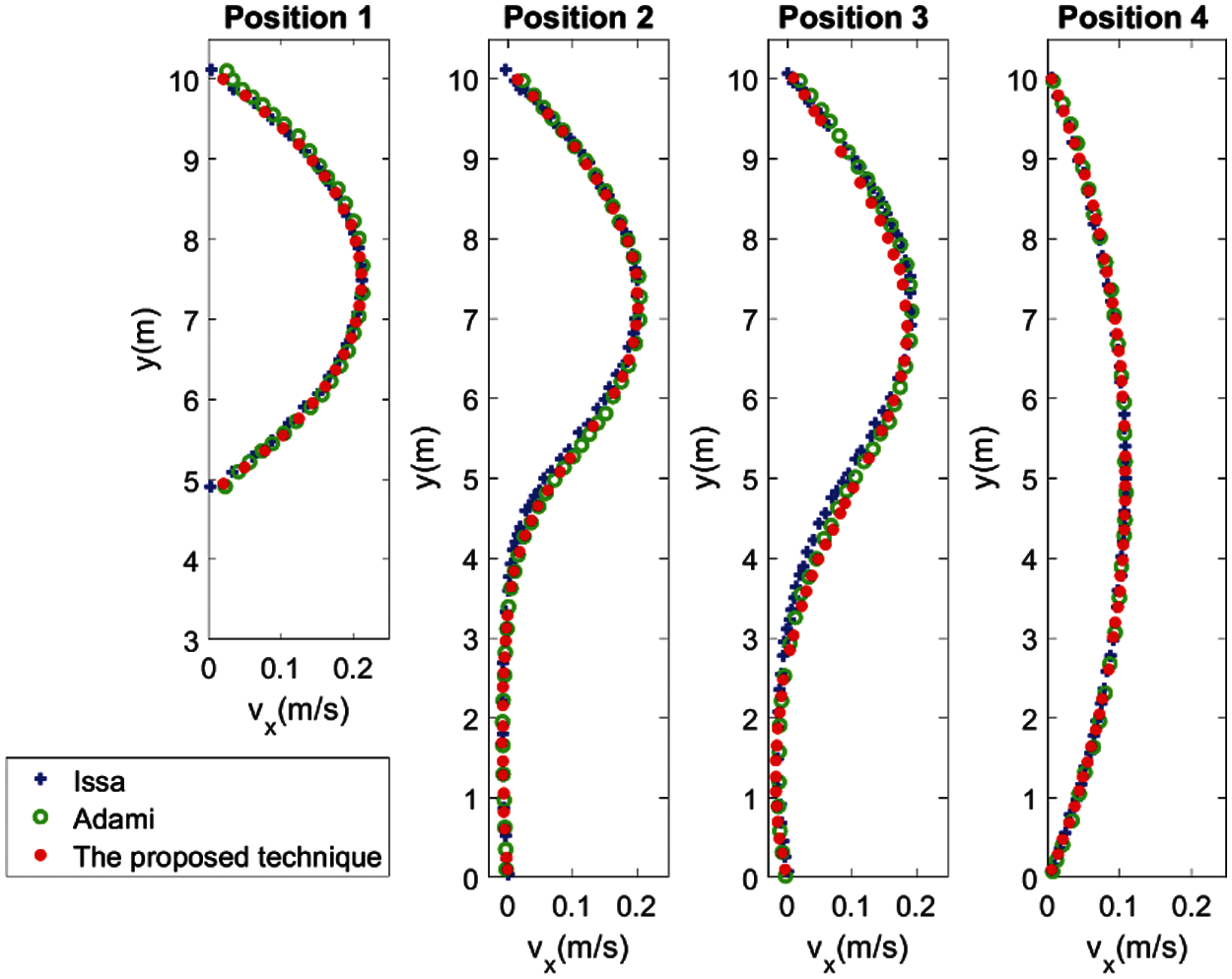
Figure 17: Comparison of the axial velocities at four different marked positions, P1–P4, for Re=100

Fig. 18 depicts the variation of fluid particles in the computational time. The number of fluid particles is 26160 at the beginning and it reaches to 26281 particles at Re=100. The percentage of mass error is 0.46%.

Figure 18: Time history of number of particles in the entire computational process

5  Conclusions

In this paper, we developed a simplified approach of open boundary conditions. Taking advantage of the δ+-SPH scheme, the proposed technique is simple to implement but is effective and robust in test cases. The approach is classified into sets of fluid, wall, inflow, and outflow particles, as in most inflow/outflow algorithms. The inflow/outflow information is treated as fluid particles to ensure appropriate evolution to the flow field instead of using a renormalization process referencing the fluid particles. The values of new inflow particles are copied from the shifted particles, and the differences are corrected using the PST.

The numerical tests demonstrate that the proposed technique obtains good results with a high agreement with the reference solutions. The first test case demonstrated the stability of the flow field over a sufficiently long time with the MSEP value of the velocity field being approximately 0.1%. Given this stability, we compressed the computational domain to a lower resolution in a second test case to demonstrate the high accuracy of the simulation. The third test case examined the flexibility of the inflow boundary conditions to prescribed or non-prescribed values. This case developed results well suited to the wall boundary and the evolution of the flow field. The performance of the results demonstrated the versatility of the proposed technique. Overall, the proposed technique has addressed the information on inflow/outflow particles without extrapolation from the fluid zone.

One of the limitations is that particles in the fluid zone can move across the borders of inflow zones in case of flow reversion. This issue is pointed out also in [6] and a decent solution is given in the paper. We expect to improve this issue in future work.

Acknowledgement: This research was supported by the Ministry of Education, Culture, Sports, Science and Technology (MEXT), Japan.

Funding Statement: The authors received no specific funding for this study.

Conflicts of Interest: The authors declare that they have no conflicts of interest to report regarding the present study.

This work is licensed under a Creative Commons Attribution 4.0 International License, which permits unrestricted use, distribution, and reproduction in any medium, provided the original work is properly cited.