| Computer Modeling in Engineering & Sciences |
DOI: 10.32604/cmes.2021.016980
ARTICLE
Fusion Fault Diagnosis Approach to Rolling Bearing with Vibrational and Acoustic Emission Signals
1School of Aeronautics, Northwestern Polytechnical University, Xi’an, 710072, China
2Department of Aeronautics and Astronautics, Fudan University, Shanghai, 200433, China
*Corresponding Author: Yunwen Feng. Email: fengyunwen@nwpu.edu.cn
Received: 16 April 2021; Accepted: 11 May 2021
Abstract: As the key component in aeroengine rotor systems, the health status of rolling bearings directly influences the reliability and safety of aeroengine rotor systems. In order to monitor rolling bearing conditions, a fusion fault diagnosis method, namely empirical mode decomposition (EMD)-Mahalanobis distance (E2MD) and improved wavelet threshold (IWT) (E2MD-IWT) for vibrational signals and acoustic emission (AE) signals is developed to improve the diagnostic accuracy of rolling bearings. The IWT method is proposed with a hard wavelet threshold and a soft wavelet threshold. Moreover, it is shown to be effective through numerical simulation. EMD is utilized to process the original AE signals for rolling bearings so as to generate a set of components called intrinsic modes functions (IMFs). The Mahalanobis distance (MD) approach is introduced in order to determine the smallest MD between the original AE signal and IMF components. Then, the IWT approach is employed to select the IMF components with the largest MD. It is demonstrated that the proposed E2MD-IWT method for vibrational and AE signals can improve rolling bearing fault diagnosis, beyond its ability to effectively eliminate noise signals. This study offers a promising approach to fault diagnosis for rolling bearings in aeroengines with regard to vibration signals and AE signals.
Keywords: Empirical mode decomposition; mahalanobis distance; improved wavelet threshold; rolling bearings
Bearings are important components in industrial applications, such as gas turbines and aeroengines. In order to ensure bearings are reliable and safe, condition monitoring should be used, which has large economic value and social benefits. As of 2021, numerous condition monitoring techniques have been developed, including acoustical emission (AE)-based monitoring techniques and vibrational-based monitoring techniques [1–3]. The AE method is widely used in fault diagnosis [4–6], when traditional linear filtering method cannot effectively denoise signals. In order to tackle this problem, the wavelet approach is applied to denoise and extract the features from AE signals [7]. The wavelet analysis approach has good local in time-frequency domain, which helps with unstable signal analysis. However, the denoising effect of wavelet analysis is closely related to the characteristics of signals and the selection of wavelet basis function and decomposition layers. In order to resolve this problem, Huang et al. [8] developed the empirical mode decomposition (EMD) method to decompose signals into numerous intrinsic mode components (IMF). Wavelet transformation requires a wavelet basis function, while decomposition depends on the basis function [8]. The EMD method can linearly and stably handle nonlinear and unstable signals. Nevertheless, EMD is an adaptive signal processing method which obtains adaptive basis functions for different signals [9–13]. In this case, EMD cannot process complex nonlinear and unstable signals due to modal aliasing with intermittent events and missing frequencies [14].
A new method, the periodic process, was developed by combining wavelet denoising and EMD. Yang and An analyzed the vibration signals of wind turbine gear boxes through wavelet transformation to address high-frequency signals via EMD [15]. Kedadouche et al. [16] used EMD and wavelet transformation to decompose acoustical signals into IMFs. The soft threshold method was applied to each IMF to further denoise them. This method is more effective than using the soft threshold method on its own. Using an improper wavelet threshold can have a negative impact on denoising. In this case, an improved wavelet threshold denoising method is developed in order to enhance the ability of EMD to denoise [17]. This work offers a promising approach to improving the fault diagnosis of rolling bearings using vibrational and AE signals. By integrating EMD, the Mahalanobis distance method and an improved wavelet threshold method, this paper develops a fusion fault diagnosis method, called empirical mode decomposition (EMD)-Mahalanobis distance (E2MD) and improved wavelet threshold (IWT) (E2MD-IWT), which enhance the diagnostic accuracy of rolling bearings taking vibrational signals and acoustic emission (AE) signals into account. The IWT method, which is based on a hard wavelet threshold and a soft wavelet threshold, is shown to be effective through simulations. EMD is used to process the original AE signals of rolling bearings for the purpose of generating a set of components called intrinsic modes functions (IMFs). The Mahalanobis distance (MD) approach is used to select the smallest MD between the original AE signal and IMF components, while the IWT approach is adopted to determine the IMF components based on the largest MD.
The rest of this paper is organized as follows: Section 2 introduces the basic theories of the E2MD-IWT method, namely the EMD method, the MD method, the Wavelet threshold denoising method and Teager energy spectrum analysis, which are used to support the fault diagnosis of rolling bearings. In Section 3, the fault diagnosis of rolling bearings is used to validate the proposed E2MD-IWT method in terms of denoising ability and diagnostic accuracy, based on rotor fault simulation tests. Finally, Section 4 summarizes the conclusions.
2.1 Empirical Mode Decomposition (EMD) Method
As a commonly used signal processing method, empirical mode decomposition (EMD) is utilized to decompose complex signals into intrinsic mode components (IMFs). IMFs must satisfy two conditions [8]: (a) the number of zero-crossings (including the maximum and minimum points) must be equal (or differ by no more than one) across the dataset; and (b) at any point, the mean value of the upper envelope and lower envelope must both be zero on the basis of the local minima principle. For the signal x(t), the EMD procedure is as follows [18]:
Step 1: All the local extremum values (including maxima and minima) for x(t) are calculated, and then the cubic spline curve method [19] is applied to fit the upper envelope xh(t) and the lower envelope xl(t) containing the maxima and minima points, respectively.
Step 2: The average value m(t) of the upper envelope xh(t) and lower envelope xl(t) is computed by
Step 3: The difference x1(t) between the original signal x(t) and the mean value m(t) can be expressed as
Step 4: When x1(t) satisfies the IMF condition, x1(t) is the first component of x(t), i.e., the first IMF (IMF1) and denoted by c1(t). When x1(t) does not satisfy the IMF condition, Steps 1~3 are repeated until the first IMF is acquired.
Step 5: After acquiring the first IMF c1(t), the rest signal r1(t) for x(t) is given by
The rest signal r1(t) is considered the new original signal with which Steps 1~4 can again be applied until all the IMF components of x(t) are calculated. Complete decomposition is achieved when the rest signal is a non-oscillating monotone function or less than a preset value. Assuming that the original signal x(t) can be ultimately decomposed into n IMFs and a rest signal rn(t)
where ci(t) is the ith IMF which is the ith component of the original signal x(t).
The flow chart for calculting EMD for an original signal x(t) is described in Fig. 1.
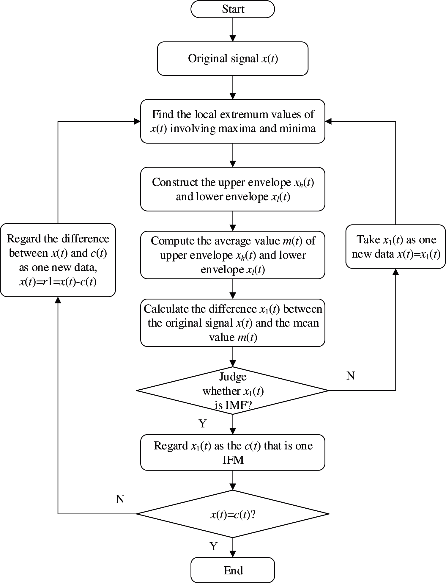
Figure 1: Flow chart for empirical mode decomposition (EMD)
2.2 The Mahalanobis Distance (MD) Method
The Mahalanobis distance (MD) method [16–18] was developed by the Indian statistician Mahalanobis, to express the covariance distance of data. The MD method is an effective method for calculating the similarity between two unknown samples. Unlike with Euclidean distance [20], MD is not affected by dimensions and not related to the measurement units used. The MD between two points can be either standardized or centralized. The MD method only considers the contacts between different characteristics, ignoring any correlation between variables [21,22]. Therefore, MD can be easily measured, making it suitable for fault detection.
The observation distance d between the sample y and the sample x with m × n is defined as
where m is the dimensional number of sample vector x; n is the number of samples; and
The covariance matrix of matrix x is
where xi is the ith element in matrix x.
By using the EMD method, a smaller MD between the original signals and IMF components can be extracted for rolling bearing faults, which is the basis of rolling bearing fault diagnosis.
2.3 The Wavelet Threshold Denoising Method
In practice, noisy signals usually appear as high frequency signals, while useful signals appear either as low frequency or more smooth signals. When signals are decomposed by wavelet, signals with noise in the high frequency wavelet cannot be eliminated. Therefore, the threshold quantization threshold is applied to process these high frequency wavelet coefficients in order to reconstruct the signals. Signal wavelet threshold denoising begins by determining the critical threshold λ. If the wavelet coefficients are smaller than the critical threshold λ, the coefficients produced by noise are removed. However, the coefficients induced by useful signals remain when the wavelet coefficients are greater than the critical threshold λ. In this case, signals are denoised via the wavelet inverse transformation of the processed wavelet coefficients. The wavelet threshold denoising method works as follows:
Step 1: Apply wavelet transformation to the signal f(t) with noise for one group of wavelet decomposition coefficients
Step 2: Handle the wavelet decomposition coefficients
Step 3: Reconstruct the estimated wavelet coefficients
As shown above, the threshold and threshold function play a crucial role in determining denoising quality [18]. The wavelet threshold denoising method was developed to choose the optimum basis function and decomposition layers for wavelet decomposition [23]. The wavelet coefficients are determined by choosing the appropriate threshold function and threshold for different wavelet dimensions. With this method, the noise in signals with high frequency wavelet coefficients can be eliminated using threshold quantization threshold processing high frequency wavelet coefficients to reconstruct the signals [24,25]. Threshold functions, including the soft threshold and hard threshold functions, are given in Eqs. (8) and (9).
The soft threshold function is given as
where sgn() is the symbol function; and Thr is the threshold.
The hard threshold function is given as
The wavelet coefficients in the soft threshold and hard threshold functions vary between the threshold and zero, due to signal distortion. In order to address this issue, this study develops an improved wavelet threshold, in which wavelet coefficients are less than the threshold and the small wavelet coefficients contain useful message in the signals. The improved threshold function is denoted by
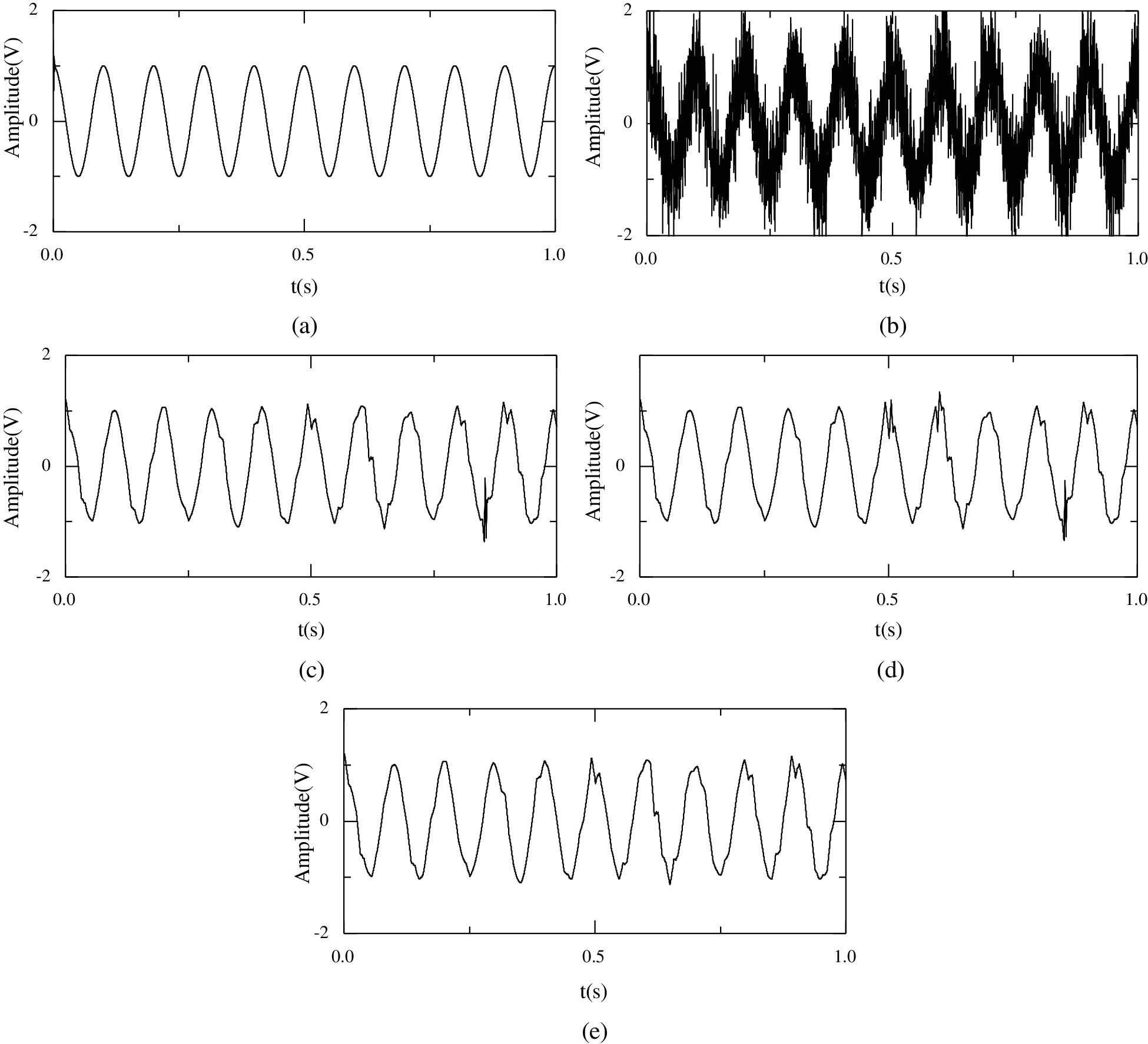
Figure 2: The original and threshold signals in the time domain with different thresholds (a) Original signal (b) Noise signal (c) Hard threshold (d) Soft threshold (e) Improved threshold
In order to validate the effectiveness of the improved wavelet threshold, a simulated signal x(t) = x0(t) + x1(t) with sample frequency 4,096 Hz and sample time 1 s is selected. x0(t) is the periodic pulse decay signal with frequency 16 Hz. In each cycle, x1(t) has the attenuation function e–1000t · cos(2π · 600t) with frequency 10 Hz. The white gauss noise is overlayed with regard to the signal x(t). The time domain origin signal, noise signal, hard threshold signal, soft threshold signal and improved threshold signal are shown in Fig. 2.
As demonstrated in Fig. 2, the hard threshold, soft threshold and improved threshold can effectively remove noise and maintain the image detail to a high standard. Moreover, the improved threshold is less distorted than the hard threshold and soft threshold. The denoising effect is also diagnosed and the results are shown in Tab. 1. As listed in Tab. 1, the improved threshold has the largest signal-to-noise ratio (SNR) and smallest mean square error (MSE), which shows that the improved threshold method has a strong denoising effect and less distortion relative to the hard threshold and soft threshold in terms of signal denoising.

2.4 Teager Energy Spectrum Analysis
The nonlinear energy tracking operator is used to analyze and track the energy of narrowband signals using a simple mathematical method [26]. In order to simplify the narration, the nonlinear energy tracing operator is abbreviated as the energy operator, denoted by Ψ. The Teager energy operator Ψ of the signal x(t) [26–29] is defined as
where
In Eq. (12), Ψ[x(n)] can be calculated for the source of the signal energy at time n using three samples. It can be seen from Eqs. (11) and (12) that the essence of the Teager energy operator is the square product of the instantaneous amplitude and the instantaneous frequency of the vibration signal. Compared with the traditional energy definition, the square product of the frequency is present in the Teager energy operator. The vibration frequency of the transient impact is higher in rolling bearings. Therefore, the output of the Teager energy operator can effectively enhance the transient impact components, and then extract the early weak fault characteristics of the rolling bearings. In this paper, the Teager energy operator is employed to extract the features of rolling bearing faults.
The bearing fault simulation test bench is shown in Fig. 3, which contains a computer, AE sensor and data collector. The bearing outer-race fault is displayed in Fig. 4, which is processed using the linear cutting method [30,31], with width 0.5 mm and depth 0.5 mm. In this study, the TMB-N204M bearing is used and its basic parameters are shown in Tab. 2. The feature frequency of the rolling bearing outer-race fault is f0 = 84 Hz for a rotating speed of 1,116 rpm, in line with Eq. (13).
where Z is the number of rollers; Dw indicates pitch diameter; Dpw denotes roll bar diameter; β expresses contact angle; and fr is the roller running frequency.
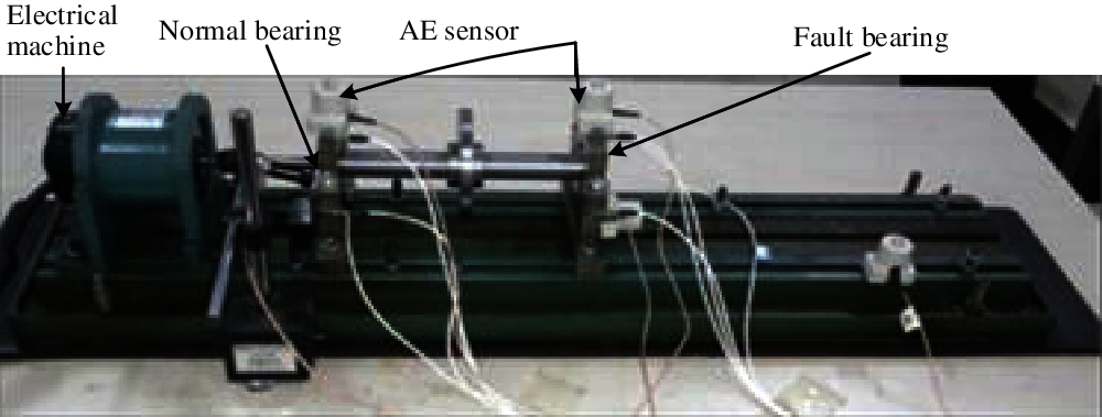
Figure 3: Simulation test bench for bearing faults
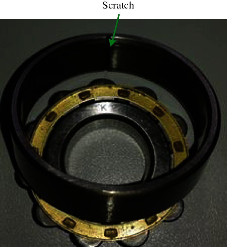
Figure 4: Bearing outer ring fault

Figs. 5 and 6 show the time domain and frequency domain graphs for the fault bearing outer ring, respectively. In Fig. 5, the obvious periodic impact failure can be seen, with interference signals departing shortly after. In Fig. 6, the natural frequency spectrum of the bearing fault is not obvious and requires further denoising.
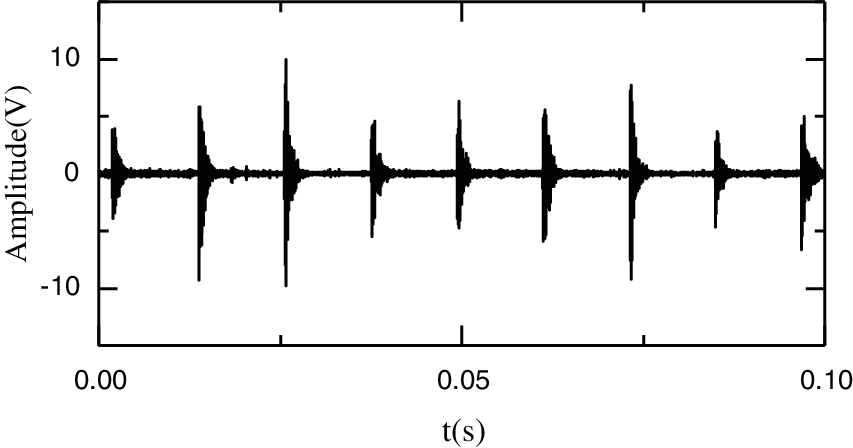
Figure 5: Time domain graph of the bearing outer ring fault
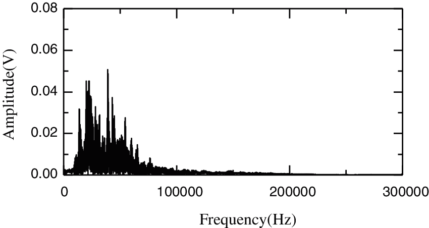
Figure 6: Frequency domain graph of the bearing outer ring fault
In order to extract obvious fault features, it is necessary to denoise the original signals of the bearing fault. EMD is applied to decompose the original signals and calculate their IMF components, as shown in Figs. 7 and 8.
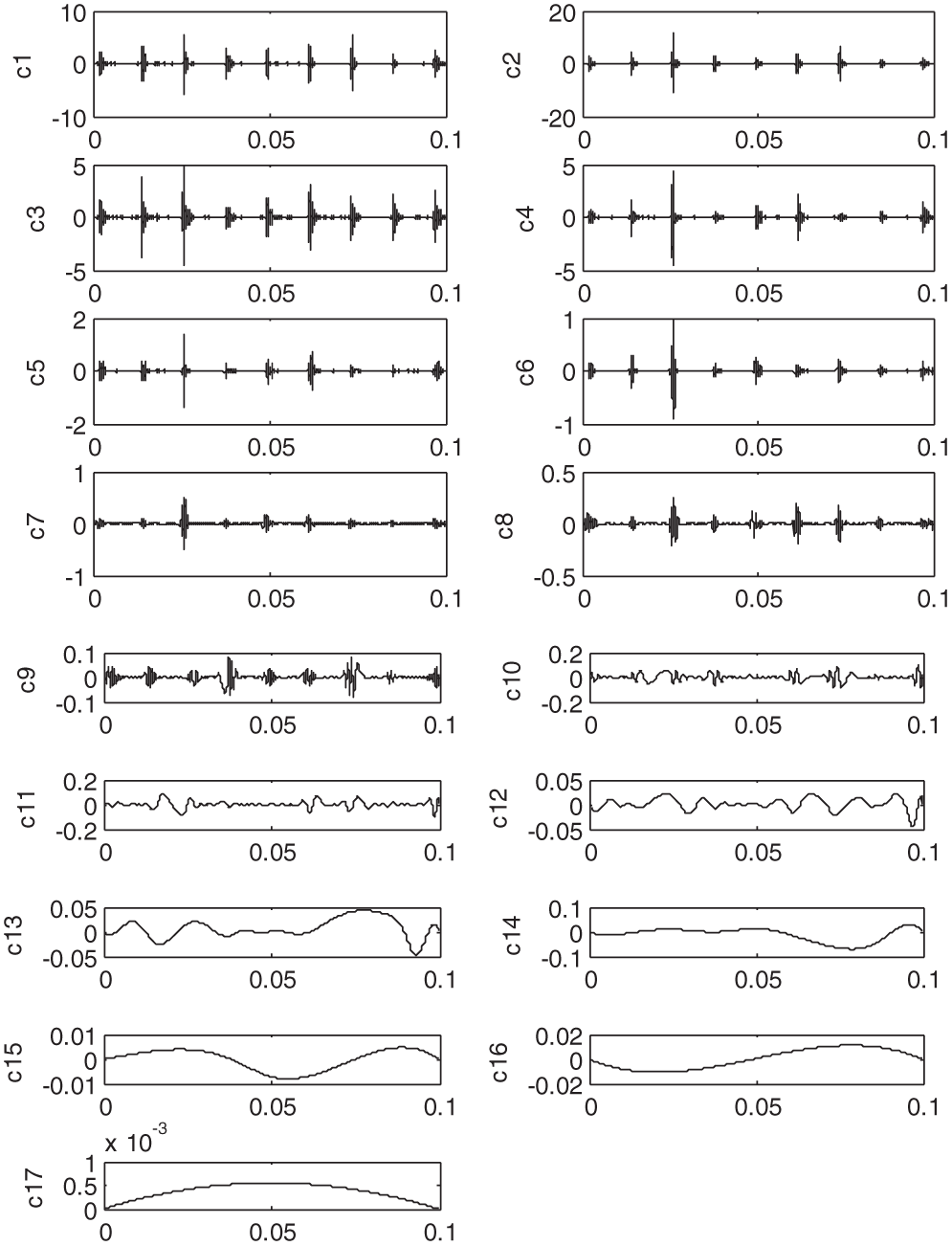
Figure 7: c1–c17 IMF components
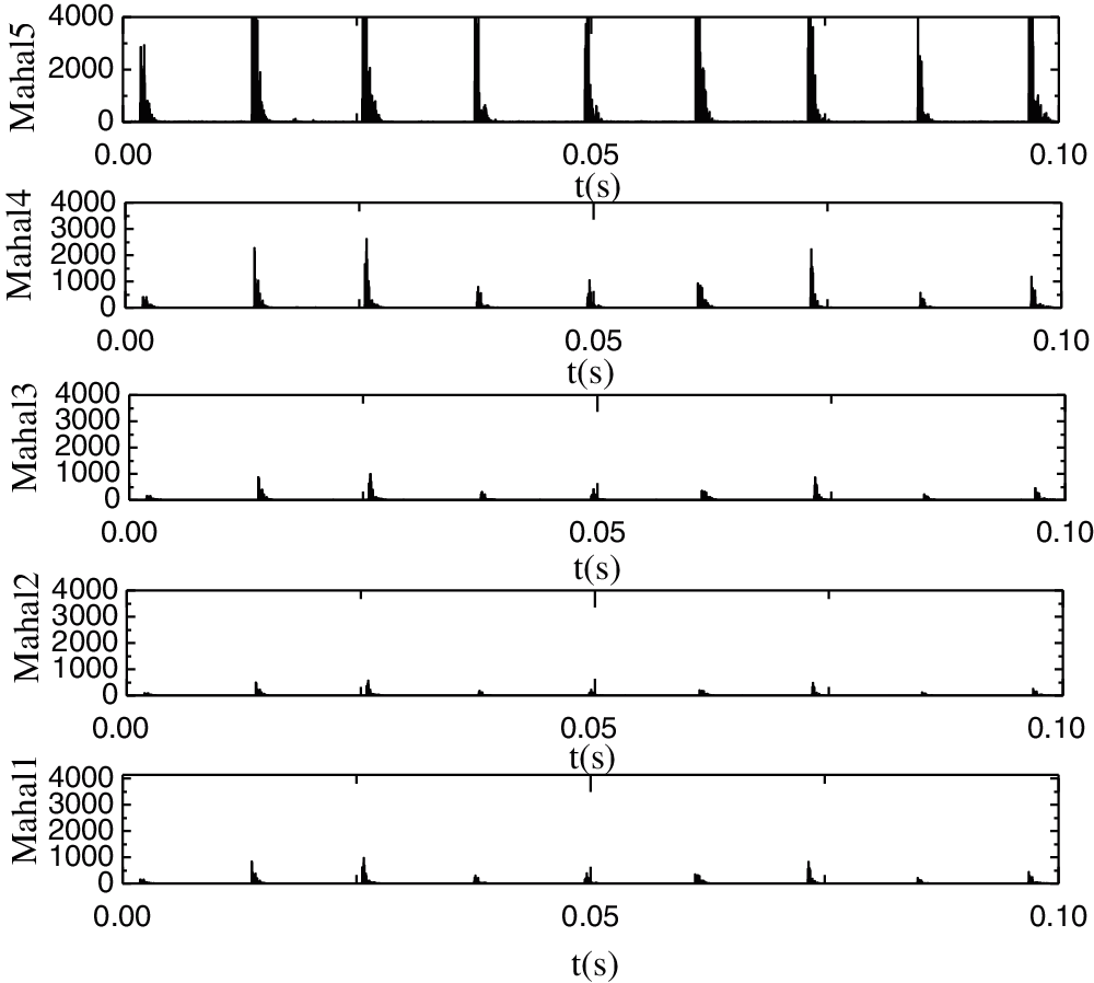
Figure 8: MD between the first five IMFs and the original signals
Fig.8 shows the MD between the first five IMFs and the original signals. As shown in Fig. 8, the peak value of Mahal2 is the lowest, while the peak values of the first five IMFs are such that Mahal2 > Mahal3 > Mahal1 > Mahal4 > Mahal5. For precision, the average MD is calculated for all the points of the first five IMFs. These are denoted by avg1, avg2, avg3, avg4 and avg5, as shown in Tab. 3. As illustrated in Tab. 3, the average values are such that avg2 > avg3 > avg1 > avg4 > avg5. Like in Fig. 8, Mahal2, Mahal3 and Mahal1 are considered the real components, while the rest are taken to be false low frequency and excluded.
The proposed improved wavelet threshold method is applied to components c1–c3. The sym5 wavelet base undergoes five-layer decomposition in order to deconstruct the five layers of the wavelet. The denoised signal is shown in Figs. 9–11.
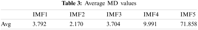
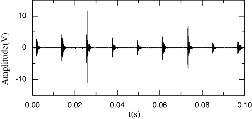
Figure 9: Denoised signal for c2
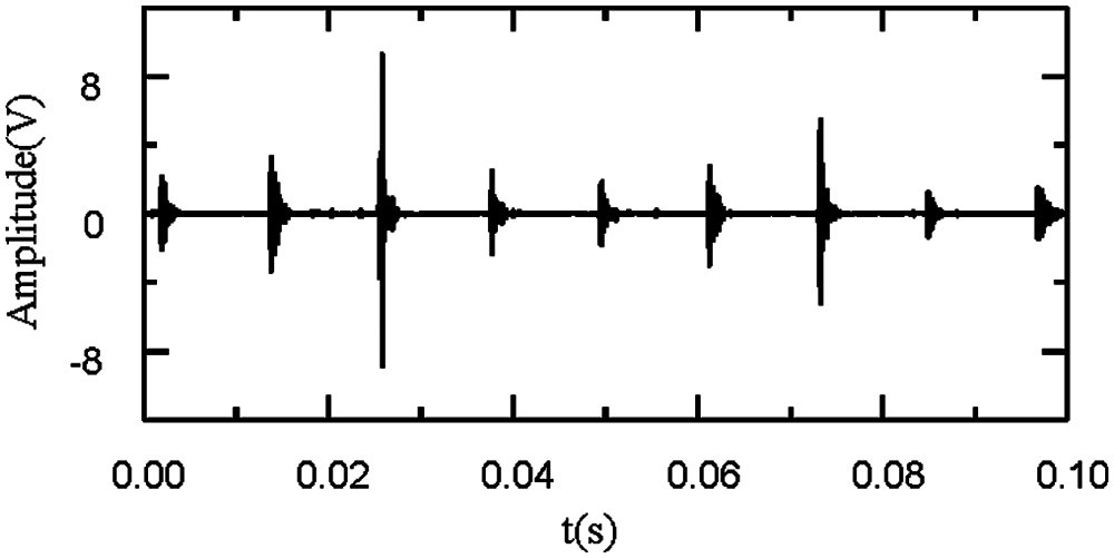
Figure 10: Denoised signal for c3
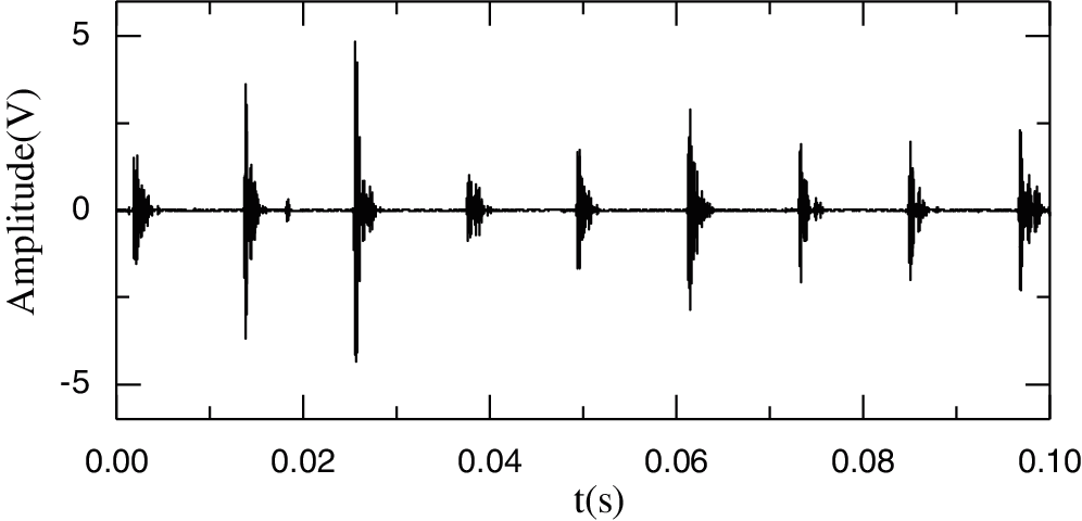
Figure 11: Denoised signal for c1
In order to determine the frequency of the bearing fault, Teager energy spectrum analysis is used to denoise components c1–c3. As shown in Fig. 12, the frequency 83.92 Hz is equal to f0 84.00 Hz as approximated in Eq. (13), which indicates that the outer rface of the bearing is broken. The amplitudes of the failure frequency in Figs. 13 and 14 are smaller than that in Fig. 12, because the MDs are greater than that in Fig. 12.
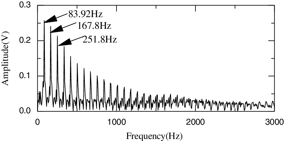
Figure 12: Teager energy spectrum for c2
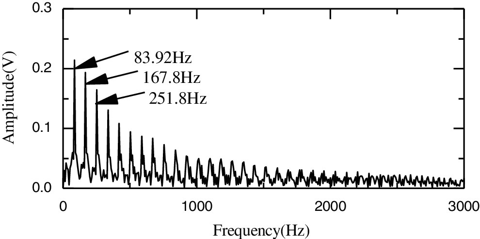
Figure 13: Teager energy spectrum for c3
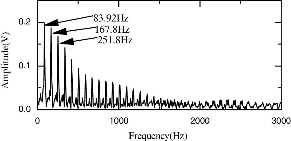
Figure 14: Teager energy spectrum for c1
In order to verify the proposed E2MD-IWT method, the Teager energy spectrum analysis method is compared in terms of signal processing. Fig. 15 presents the Teager energy spectrum analysis result for the original signal.
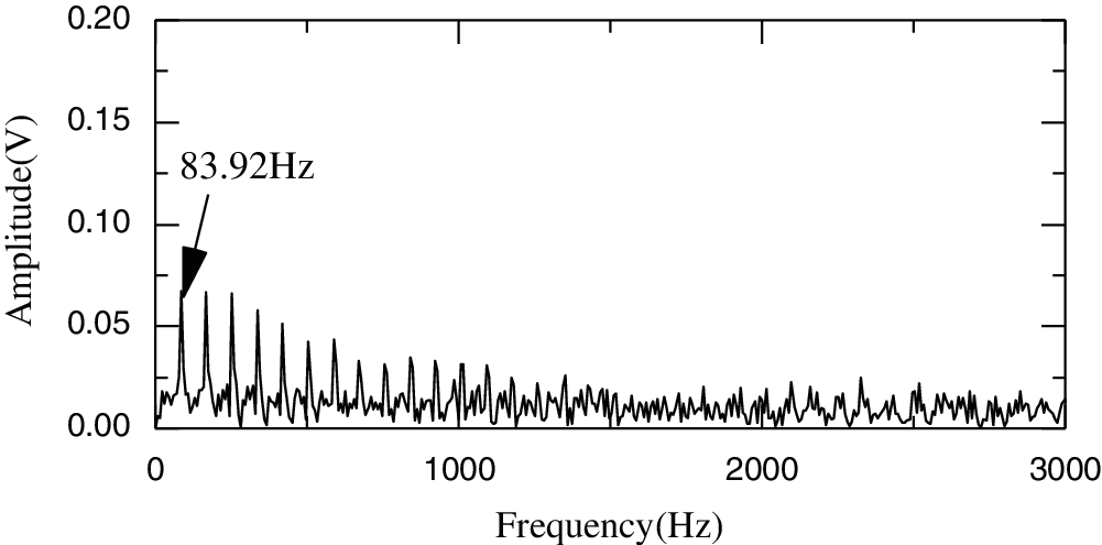
Figure 15: Teager energy spectrum analysis for the original signal
As illustrated in Fig. 15, the failure frequency 83.92 Hz also exits, but its amplitude is smaller in Figs. 12–14. As a result, there are fewer frequency multiplications than in Figs. 12–14 and weaker denoising. Therefore, the proposed E2MD-IWT method in this study is more effective and can diagnose the fault types of rolling bearings. Hence, the proposed E2MD-IWT method can effectively enhance the fault diagnosis of rolling bearings.
This study sought to develop a fusion fault diagnosis method (i.e., empirical mode decomposition (EMD)-Mahalanobis distance (MD) (E2MD) and improved wavelet threshold (IWT) (E2MD-IWT)) for vibrational signals and acoustic emission (AE) signals, for the purpose of enhancing the diagnostic accuracy of rolling bearings. The E2MD-IWT method integrates the strengths of the EMD method, the MD approach, the IWT method and the Teager energy method. When diagnosing faults with the proposed E2WD-IWT method, EMD is used to process the original AE signals of the rolling bearing so as to generate a set of components (intrinsic modes functions, IMFs). Then, the MDs of said IMFs are calculated using the MD method by selecting the smallest MD between the original AE signal and its IMF components. Meanwhile, those IMF components that have the largest MD are selected using the IWT method. The Teager energy spectrum analysis approach is applied to extract the natural frequencies of the acquired denoised fault signals. The performance of the fault diagnosis using the proposed E2MD-IWT can be summarized as follows:
(1) The improved wavelet threshold denoises better than the traditional hard wavelet threshold and soft wavelet threshold;
(2) The developed E2MD-IWT method can more precisely extract fault features and diagnose rolling bearing fault signals than direct Teager energy spectrum analysis as applied to the original AE signals;
(3) The proposed E2MD-IWT method enhances the fault diagnosis of rolling bearings with regard to denoising and feature extraction.
In future work, more parameter identification methods should be investigated for a range of signal types, such as AE signals and vibration signals, in order to support its application in engineering and further improve health status monitoring for rolling bearing in complex machinery, like aeroengines.
Funding Statement: This paper is supported by the National Natural Science Foundation of China (Grant No. 51875465) and the Civil Aircraft Scientific Research Project. The authors would like to thank them.
Conflicts of Interest: The authors declare that there are no conflicts of interest regarding the publication of this paper.
1. Fei, C. W., Choy, Y. S., Tang, W. Z., Bai, G. C. (2018). Multi-feature entropy distance approach with vibration and AE signals for process feature extraction and diagnosis of rolling bearing faults. Structural Health Monitoring, 17(2), 156–168. [Google Scholar]
2. Fei, C. W., Bai, G. C., Tang, W. Z., Ma, S. (2014). Quantitative diagnosis of rotor vibration fault using process power spectrum entropy and support vector machine method. Shock and Vibration, 2014, 957531. DOI 10.1155/2014/957531. [Google Scholar] [CrossRef]
3. Sun, D., Wang, S. D., Fei, C. W., Zhao, H., Zhang, G. C. et al. (2019). Experimental investigation on rotordynamic characteristics and rotor system stability of a novel negative dislocated seal. Shock and Vibration, 2019(8), 1–11. DOI 10.1155/2019/1780390. [Google Scholar] [CrossRef]
4. Tian, J., Wang, S. G., Zhou, J., Bai, J. Z., Ai, Y. T. et al. (2021). Fault diagnosis of inter-shaft bearing using variational mode decomposition with TAGA optimization. Shock and Vibration, 2021, 8828317. DOI 10.1155/2021/8828317. [Google Scholar] [CrossRef]
5. Tian, J., Liu, L. L., Zhang, F. L., Ai, Y. T., Wang, Z. et al. (2020). Multi-domain entropy-random forest method for the fusion diagnosis of Inter-shaft bearing faults with AE signals. Entropy, 22(1), 57. DOI 10.3390/e22010057. [Google Scholar] [CrossRef]
6. Tian, J., Ai, Y. T., Fei, C. W., Zhang, F. L., Choy, Y. S. (2019). Dynamic modeling and simulation of inter-shaft bearings with localized defects excited by time-varying displacement. Journal of Vibration and Control, 25(8), 1436–1446. DOI 10.1177/1077546318824927. [Google Scholar] [CrossRef]
7. Tian, J., Ai, Y. T., Fei, C. W., Zhao, M., Zhang, F. L. et al. (2018). Fault diagnosis of inter-shaft bearings using fusion information energy distance method. Shock and Vibration, 2018, 7546128. DOI 10.1155/2018/7546128. [Google Scholar] [CrossRef]
8. Huang, N. E., Shen, Z., Long, S. R., Wu, M. C., Shih, H. H. et al. (1998). The empirical mode decomposition and the Hilbert Spectrum for nonlinear and non-stationary time series analysis. Proceeding of Royal Society London A, 454(1971), 903–995. DOI 10.1098/rspa.1998.0193. [Google Scholar] [CrossRef]
9. Wang, L., Wang, C., Cai, Z. (1999). The diagnosis method for the rolling bearings tiny fault based on wavelet. Chinese Journal of Applied Mechanics, 16(2), 95–99. DOI CNKI:SUN:YYLX.0.1999-02-015. [Google Scholar]
10. Tang, Y., Sun, Q. (2002). Study on vibration signal singularity analysis by wavelet for rolling element bearing defect detection. Journal of Vibration, 15(1), 111–113. DOI 10.1002/mop.10502. [Google Scholar] [CrossRef]
11. Peng, Z. K., He, Y. Y., Lu, Q., Lu, W. X., Chu, F. L. (2003). Using wavelet method to analyze fault features of rub rotor in generator. Proceedings of the Chinese Society of Electrical Engineering, 23(5), 75–79. DOI 10.3321/j.issn:0258-8013.2003.05.017. [Google Scholar] [CrossRef]
12. Yang, S. X., Hu, J. S., Wu, Z. T., Yan, G. B. (2003). The comparison of vibration signals time-frequency analysis between EMD-based HT and WT method in rotating machinery. Proceedings of the Chinese Society of Electrical Engineering, 23(6), 102–107. DOI 10.3321/j.issn:0258-8013.2003.06.020. [Google Scholar] [CrossRef]
13. Fan, C., Zhang, L., Wang, Z., Ji, S. (2016). Research of fault diagnosis of rolling bearings based on EMD and power spectrum analysis method. Journal of Mechanical Strength, 28(4), 628–631. DOI 10.3321/j.issn:1001-9669.2006.04.033. [Google Scholar] [CrossRef]
14. Lu, C., Fei, C. W., Feng, Y. W., Zhao, Y. J., Dong, X. W. (2021). Probabilistic analyses of structural dynamic response with modified Kriging-based moving extremum framework. Engineering Failure Analysis, 125, 105398. DOI 10.1016/j.engfailanal.2021.105398. [Google Scholar] [CrossRef]
15. Yang, Q., An, D. (2013). EMD and wavelet transform based fault diagnosis or wind turbine gear box. Advances in Mechanical Engineering, 5(11), 212836. DOI 10.1155/2013/212836. [Google Scholar] [CrossRef]
16. Kedadouche, M., Thomas, M., Tahan, A. (2016). A comparative study between empirical wavelet transforms and empirical mode decomposition methods: Application to bearing defect diagnosis. Mechanical Systems and Signal Processing, 81(15), 88–107. DOI 10.1016/j.ymssp.2016.02.049. [Google Scholar] [CrossRef]
17. Kagan, A., Li, B. (2008). An identity for the Fisher Information and mahalanobis distance. Journal of Statist Plann Inference, 138(12), 3950–3959. DOI 10.1016/j.jspi.2008.02.017. [Google Scholar] [CrossRef]
18. Moti, L. T. M. Q. I., Sahar, B. Q. (2010). Mahalanobis distance under nonnormality. A Journal of Theoretical and Applied Statistics, 43(3), 275–280. DOI 10.1080/02331880903043223. [Google Scholar] [CrossRef]
19. Krishna, A. V. N., Narayana, A. H., Vani, K. M. (2016). Window method based cubic spline curve public key cryptography. International Journal of Electronics and Information Engineering, 4(2), 94–102. [Google Scholar]
20. Keshtegar, B., Bagheri, M., Fei, C. W., Lu, C., Taylan, O. et al. (2021). Multi-extremum modified response basis model for nonlinear response prediction of dynamic turbine blisk. Engineering with Computers, 35(6), 487. DOI 10.1007/s00366-020-01273-8. [Google Scholar] [CrossRef]
21. Han, L., Chen, C., Guo, T. Y., Lu, C., Fei, C. W. et al. (2021). Probability-based service safety life prediction approach of raw and treated turbine blades regarding combined cycle fatigue. Aerospace Science and Technology, 110(7), 106513. DOI 10.1016/j.ast.2021.106513. [Google Scholar] [CrossRef]
22. Fei, C. W., Liu, H. T., Rhea, P. L., Choy, Y. S., Han, L. (2021). Hierarchical model updating strategy of complex assembled structures with uncorrelated dynamic modes. Chinese Journal of Aeronautics, 95(11), 700. DOI 10.1016/j.cja.2021.03.023. [Google Scholar] [CrossRef]
23. Donoho, D. L. (1995). De-noising by soft-thresholding. IEEE Transactions on Information Theory, 41(3), 613–627. DOI 10.1109/18.382009. [Google Scholar] [CrossRef]
24. Barri, A., Dooms, A., Schelkens, P. (2012). The near shift-invariance of the dual-tree complex wavelet transform revisited. Journal of Mathematical Analysis and Applications, 389(2), 1303–1314. DOI 10.1016/j.jmaa.2012.01.010. [Google Scholar] [CrossRef]
25. Wang, C. L., Zhang, C. L., Zhang, P. T. (2012). Denoising algorithm based on wavelet adaptive threshold. Physics Procedia, 24(A), 678–685. DOI 10.1016/j.phpro.2012.02.100. [Google Scholar] [CrossRef]
26. Maragos, P., Kaiser, J. F., Quatieri, T. F. (1993). On amplitude and frequency demodulation using energy operators. IEEE Transaction on Signal Processing, 41(4), 1532–1550. DOI 10.1109/78.212729. [Google Scholar] [CrossRef]
27. Maragos, P., Kaiser, J. F., Quatieri, T. F. (1993). Energy separation in signal modulations with application to speech analysis. IEEE Transaction on Signal Processing, 41(10), 3024–3051. DOI 10.1109/78.277799. [Google Scholar] [CrossRef]
28. Ma, J., Wu, J. D., Wang, X. D. (2018). Incipient fault feature extraction of rolling bearings based on the MVMD and teager energy operator. ISA Transactions, 80(8), 297–311. DOI 10.1016/j.isatra.2018.05.017. [Google Scholar] [CrossRef]
29. Fei, C. W., Liu, H. T., Li, S. L., Li, H., An, L. Q. et al. (2021). Dynamic parametric modeling-based model updating strategy of aeroengine casings. Chinese Journal of Aeronautics, 24(7), 2137. DOI 10.1016/j.cja.2020.10.036. [Google Scholar] [CrossRef]
30. Kang, H., Cho, J. W., Park, J. Y., Jang, J. S., Kim, J. H. et al. (2016). A new linear cutting machine for assessing the rock-cutting performance of a pick cutter. International Journal of Rock Mechanics and Mining Sciences, 88, 129–136. DOI 10.1016/j.ijrmms.2016.07.021. [Google Scholar] [CrossRef]
31. Lu, C., Fei, C. W., Li, H., Liu, H. T., An, L. Q. (2020). Moving extremum surrogate modeling strategy for dynamic reliability estimation of turbine blisk with multi-physics fields. Aerospace Science and Technology, 106(2), 106112. DOI 10.1016/j.ast.2020.106112. [Google Scholar] [CrossRef]
 | This work is licensed under a Creative Commons Attribution 4.0 International License, which permits unrestricted use, distribution, and reproduction in any medium, provided the original work is properly cited. |