Traffic Flow Statistics Method Based on Deep Learning and Multi-Feature Fusion

Mu, Liang; Zhao, Hong; Li, Yan; Liu, Xiaotong; Qiu, Junzheng; Sun, Chuanlong

doi:10.32604/cmes.2021.017276

College of Mechanical and Electrical Engineering, Qingdao University, Qingdao, 266071, China
*Corresponding Author: Hong Zhao. Email: qdlizh@163.com
Received: 28 April 2021; Accepted: 11 August 2021

Abstract: Traffic flow statistics have become a particularly important part of intelligent transportation. To solve the problems of low real-time robustness and accuracy in traffic flow statistics. In the DeepSort tracking algorithm, the Kalman filter (KF), which is only suitable for linear problems, is replaced by the extended Kalman filter (EKF), which can effectively solve nonlinear problems and integrate the Histogram of Oriented Gradient (HOG) of the target. The multi-target tracking framework was constructed with YOLO V5 target detection algorithm. An efficient and long-running Traffic Flow Statistical framework (TFSF) is established based on the tracking framework. Virtual lines are set up to record the movement direction of vehicles to more accurate and detailed statistics of traffic flow. In order to verify the robustness and accuracy of the traffic flow statistical framework, the traffic flow in different scenes of actual road conditions was collected for verification. The experimental validation shows that the accuracy of the traffic statistics framework reaches more than 93%, and the running speed under the detection data set in this paper is 32.7FPS, which can meet the real-time requirements and has a particular significance for the development of intelligent transportation.

Keywords: Deep learning; multi-target tracking; kalman filter; histogram of oriented gradient; traffic flow statistics

With the continuous popularization of automobiles, traffic congestion, emission pollution, and traffic accidents are becoming more and more prominent in traffic, and people's demand for intelligent transportation [1,2] is also increasing. The traffic flow and conditions of the actual road provide precious information for traffic management, The results of traffic flow statistics need to be further analyzed, and it is necessary to distinguish between different vehicle types and running directions. At present, the traditional traffic flow statistics methods include geomagnetic coils, microwave and infrared detectors, and other counting devices. However, these devices have certain limitations in both installation cost and counting accuracy. In recent years, many scholars have studied and analyzed the traffic flow statistical framework based on computer vision [3]. This method can effectively make up for the problems of high cost, low precision, and inconvenient maintenance of traditional methods. In addition, other functions can be added to the framework, such as the detection of traffic accidents and violations, and the collection of speed, etc. With the continuous development of computer technology, it has become possible to integrate many functions into a video monitor, which provides the impetus for the rapid development of intelligent transportation.

TFSF is divided into detection, tracking, and statistics modules. Target detection [4,5] module is the first step on the traffic flow information, get the location of the object and classification, provide the basis for later tracking module, accurate target detection can greatly improve the performance of tracking module. Therefore, the latest YOLO V5 detection algorithm is adopted [6]. By reference, it is known that the algorithm has higher detection accuracy and speed.

Target detection based on deep learning [7,8] is mainly divided into two types: two-stage and one-stage. The two-stage generates several candidate boxes on the feature map and then classifies and regresses the targets in the candidate boxes through convolution; One stage is to conduct classification regression directly on the feature graph and the YOLO series algorithm [9] in this paper belongs to this category. Girshick et al. [10,11] successively proposed Region Convolutional Neural Network (R-CNN) and Fast Region Convolutional Neural Network (FAST R-CNN). R-CNN network model has a complex structure and slow training speed, FAST R-CNN is put forward on the basis of its shortcomings to simplify the network model and improve the speed of network detection and training; Liu et al. [12] proposed a Single Shot Multibox Detector (SSD), which greatly improved the detection speed by uniformly extracting the specified area.

At present, the mainstream Tracking frameworks are all based on tracking-by-detection, that is, Tracking based on target Detection. Zeng et al. [13] proposed a method that takes the detection results of the HOG classifier as image evidence in view of the relationship between multiple targets. Mekonnen et al. [14] proposed a method to evaluate the tracking method on the common dataset, and the results showed that the SORT algorithm performed an excellent effect in the paper. The tracking framework adopted in this paper is DeepSort [15], which is highly regarded in the algorithm industry, SORT algorithm ignores the shortcoming of surface features of detected objects, and DeepSort uses more reliable measures instead of correlation measures on its basis. Given the complex traffic scene and the tendency of the target to appear nonlinear motion, this paper uses the EKF [16] to replace the KF [17] in the original DeepSort algorithm to solve the problems such as low tracking accuracy and insufficient robustness of the original algorithm in the case of the nonlinear target. Serious vehicle mutual occlusion phenomenon exists in traffic and cascading, and IOU matching of the original DeepSort algorithm cannot handle this problem well. In this paper, HOG [18] features are added to conduct apparent modeling of detected vehicles. It can effectively solve the problem of target loss when tracking.

TFSF is built based on the position of the target and the direction of the movement track, the target detection algorithm using deep learning makes better use of the target features, the adoption of this method can be more accurate and detailed statistics of traffic flow, in addition, the algorithm eliminates the interference of useless information and can run efficiently for a long time to meet the real-time requirements of intelligent transportation. The framework is highly exploitable in the later stage and can integrate many functions. This framework can provide a theoretical basis for the development of intelligent transportation systems.

In this part, the self-made Traffic Statistics Test Dataset (TSTD) is made public for the convenience of scholars. This data set is used to test the TFSF built in this paper, which can be downloaded from the following link: https://pan.baidu.com/s/1LgqTLy0yPla7jVfEbWLe8A, the code is 7lgt.

The experimental scenes in this paper are one-way and two-way lanes, as shown in Fig. 1, which are the main scenes of urban roads, and the research on this scene is universal to a certain extent. Data collection is mainly completed by the combination of the self-made dataset and network dataset. Camera Canon EOSM50 is used in the self-made dataset, and the installation position and angle are the same as the traffic control department camera. The dataset contains a variety of complex, realistic scenes, which can be divided into daytime, rainy day, and night. The dataset is used to verify the generalization ability and robustness of TFSF.

Vehicle Detection Dataset (VDD) is mainly to get more in line with the actual situation of training, improve the accuracy of target detection, so the collection in city road scene, a total of 4500 RGB images, each image has a corresponding mark, the content of the annotation includes the type of the target and the bounding box coordinates, to 4000 copies of these as a training set, the rest of 500 as a validation set. According to the survey, there are mainly three types of vehicles in the urban area, namely, cars, vans, and buses. This can be downloaded from the following link: https://pan.baidu.com/s/1lK_D_mdneE17q7pTzCeouQ; the code is ac85.

Fig. 2 shows the three types and six randomly selected pictures from each category.

The vehicle detection involved in this paper is an application of a target detection algorithm. At present, vehicle detection mainly uses traditional machine learning and deep learning methods. With the rapid development of computer technology, target detection methods based on deep learning have made great progress and are far superior to traditional algorithms in precision, speed, and application.

In deep learning to YOLO as the representative of the better performance of regression-based detection methods, where the latest YOLO V5 algorithm compared to previous generations of YOLO algorithm in flexibility and speed has been dramatically improved, this can meet the field of traffic flow statistics requirements for real-time, but in the accuracy is slightly weaker than YOLO V4 [19]. There are four types of YOLO V5 target detection networks: YOLO V5s, YOLO V5m, YOLO V5l, and YOLO V5x. Fig. 3 shows the network structure of YOLO V5s. The number of residual component dependent and convolution kernels increases gradually. With the increase of network depth, the capability of feature extraction and feature fusion of the model increases gradually, but the speed of training and testing also slows down. According to literature reference, the YOLO V5s network is the network with the smallest depth and the smallest width of the feature graph in the YOLO V5 series. The following three kinds of the network are deepened and broadened on this basis, YOLO V5s network combines good detection accuracy and extremely high speed, so the YOLO V5s network model is used for target detection, and its network structure is shown in the figure below:

YOLO V5 model is mainly divided into four parts, Input, Backbone, Neck, Prediction. The Input is divided into three parts: Mosaic data enhancement, adaptive anchor frame calculation, and adaptive image scaling; Backbone is divided into two structures, Focus structure is mainly to slice the image operation, CSP structure is mainly from the perspective of network structure design to solve the reasoning from the calculation of a large number of problems; Neck is FPN+PAN structure to strengthen network feature fusion; Prediction uses the GIOU_LOSS function, which is used to estimate the recognition loss of the detection box.

The main task of target tracking is to connect the detection target between two frames, number the target, obtain the target trajectory, and provide a data basis for TFSF. Among many target tracking algorithms, the DeepSort algorithm has high robustness and real-time performance, DeepSort algorithm is a classic representative of tracking-by-detection. This algorithm adds depth features and adds rules for box matching through the appearance model. This method can alleviate the occlusion problem to some extent and reduce the number of ID switching. It is most suitable for multi-target tracking tasks in complex traffic scenarios. The DeepSort algorithm is mainly composed of feature extraction, feature matching and position prediction modules. In this paper, the HOG of vehicles are considered to be fused into the algorithm, and the apparent modeling of vehicles has been solved to improve the accuracy of target tracking by solving the problems of target loss caused by vehicles in scene light changes, overlapping occlusion and turning. In addition, the location prediction module of the tracking algorithm has an important impact on the performance of the algorithm. The vehicle trajectory in the traffic scenario is non-linear, and the KF in the original algorithm is suitable for linear systems, and the prediction accuracy is not high for non-linear systems, Switching to the EKF for non-linear systems with high computational speed.

The traffic scene is complex and changeable [20], the mutual shielding between vehicles is serious, and the turning of the target and partial departure from the video area will quickly lead to the failure of the tracking task, and it becomes more difficult to accurately track the target in the peak period of vehicle travel.

HOG is a feature descriptor used in computer vision and image processing for target detection. The feature is composed by calculating a histogram of the gradient direction of a statistical image region, with the gradients mainly distributed in the edge regions. The feature provides a good description of the appearance and shape of a local target. Three images of three randomly selected vehicle types can be computed and visualized for HOG using the Skimage and Opencv packages in python, Fig. 4 shows HOG feature maps of the three categories of vehicles extracted.

The original DeepSort algorithm will match the unmatched Detections and Tracks only IOU after cascading matching, which is not enough to solve the matching problem of the same target between frames. In order to solve this problem, the HOG is fused in the algorithm to match the targets between different frames. The experiment proves that the average cost of extracting the HOG of the detection box is only 1ms, and the calculation is simple and almost does not consume computing power during the matching. Fig. 5 is the flow chart of the improved tracking algorithm:

All initial frames are first detected and the ID number is initialized, KF is used to predict the state parameters of the next frame, and Hungarian matching is performed according to CNN, HOG, and IOU of the prediction box and the detection box of the next frame, preset the appropriate threshold, judge characteristic relationship between distance and the size of the set threshold, As long as one of the three matches, It will enter the update stage of KF. If the Tracks are not successfully matched for T times, Tracks will be considered to have left the video and will be deleted, Detections that are not successfully matched will be given a new ID number. After all the Detections and Tracks are processed, they will enter the matching and updating link of the next frame.

KF is a kind of linear equation of state, through the input and output observation data, estimate the optimal system state. For nonlinear systems, the prediction effect of KF is poor, and KF in the DeepSort algorithm is replaced by EKF. The EKF linearizes the nonlinear system, and it mainly uses the first-order Taylor series to construct an approximately linear function by obtaining the slope of the nonlinear function at the Mean and then carries out KF on the approximate function. Therefore, this algorithm is suboptimal filtering. Because of the approximate function adopted by EKF, there is bound to be some error, but for traffic statistics which requires high real-time performance, the simplicity and speed of calculation become very necessary.

where k is discrete-time, and the state of the system at time k is expressed as X(k)∈Rn; Z(k)∈Rn is the observed value of the corresponding state; G(k) is the noise-driven matrix; W(k) is process noise; V(k) is the observation noise.

The system state equation obtained by the first-order Taylor expansion of the nonlinear function is as follows:

where, Φ is the state transition matrix, and φ is the non-random external action term added to the state equation.

where H is the observation matrix, and y is the non-random external interaction term added to the observation equation.

The first-order linearization equation is used to solve the state transition matrix and observation matrix:

In view of the traffic environment in this paper, EKF algorithm is applied to the vehicle trajectory prediction in this scene to test the accurate rate of EKF algorithm in the nonlinear system. The average accuracy of trajectory prediction of this algorithm is calculated to judge the quality of the algorithm, and the formula is as follows:

In the formula, Ave_pre represents the average accuracy of the EKF algorithm to predict the trajectory, which is used to evaluate the algorithm. Num is the total number of track points; dis is the calculation formula of the distance between two coordinate points; Max_error is the maximum allowable error of trajectory prediction in this section.

Fig. 6 shows the EKF simulation experiment of the movement trajectory of the turning vehicle. After calculating the formula, the average prediction accuracy of the EKF algorithm reaches more than 99%, so the accuracy of the algorithm meets the application requirements.

The TFSF built in this paper is suitable for several common scenes in the traffic field, as shown in Fig. 1. Due to the complexity of the traffic scene and the uncertainty of the direction of vehicle movement, the most useful and simplest information can be used to judge traffic statistics. In this way, the real-time performance of intelligent transportation can be satisfied, and the interference of useless information can be reduced.

When an ID appears for the first time, record the center point position (x,y)first, then when the ID passes through the set detection line will again record the center point (x,y)end, according to the center points of the two records, a vector direction can be calculated to determine the movement direction of the ID, Recorded_ID is the ID that has been counted, first read whether the ID is in Recorded_ID. If not, it will be counted according to the category of the tracking detection box and the direction of travel. If it has been counted then the operation will not be carried out; In the continuous traffic statistics, the IDs in the Recorded_ID will become more and more. In the later stage, TFSF will have a huge amount of computation and consume computational power. Therefore, when an ID drives out of the video area, the ID will be deleted from the Recorded_ID to ensure the speed and real-time performance of the algorithm.

The overall methodology flow chart is shown in the figure. The method in this paper transfers each frame of video or camera to the algorithm to carry out the process of detection, tracking, and counting until the counting task is completed. Fig. 8 shows flowchart of overall methodology.

The framework was built using Python3.7 and PyTorch1.7.0, Cuda10.1, Cudnn7.4.1, hardware configuration CPU is i7–10700k CPU@3.00 GHz, a single NVIDIA GeForce RTX2080Ti with 12G video memory, 4352 CUDA cores, 32G of running memory, and Ubuntu as the operating system. Also, for the threshold settings, the most effective threshold configuration was obtained through experimental testing: the confidence level was set to 0.4, the IOU matching threshold is set to 0.5, and the HOG matching threshold was set to 0.5.

Fig. 9 shows the change of the three Loss during the training process of the YOLO V5s model based on the data set constructed in this paper, from which it can be seen that the values of the three Loss tend to stabilize around 800 iterations. At this point, the optimal weights can be obtained.

TP (True Positives), divided into positive samples, and divided right; TN (True Negatives), divided into negative samples, and separated correctly; FP (False Positives), divided into positive samples, and divided wrong; FN (False Negatives), divided into negative samples, and divided wrong.

For a specific classification, take a value every 0.05 from 0.5 to 0.95 as the IOU threshold of the prediction box, calculate the recall rate and accuracy under all the thresholds, and draw the P-R curve as the abscissa and ordinate. The area under the curve is the AP value of the current classification. The mAP value is the average of the AP values for all categories. The calculation method is as follows:

In the formula, I represent the number of the current classification, n represents the total number of categories, and precision(recall) represents the value of accuracy under the current recall rate.

AP refers to the combination of Precision and Recall because Precision represents the prediction ability that the target hit can pass the threshold in all prediction results, while Recall represents the ability to cover the real target in the test set. The combination of the two can better evaluate our model. mAP is the mean of the average accuracy of each category, which is also the mean of AP of each category. FPS is how many frames per second the target network can process. FPS is simply the image refresh rate.

In order to ensure the effectiveness of the detection algorithm, the trained model was tested on the verification set, and the parameters of the network model in terms of speed and accuracy were obtained. Using different deep learning algorithms, the current state-of-the-art Faster-RCNN, SSD-512 [21] (VGG16), Centernet, and YOLO V4 were selected, using the same training set, test set, and training parameters, and the comparison results of the four algorithms are shown in Tab. 1.

The numbers after mAP and mAP50 represent the parameters to set the IOU threshold in the NMS process, IOU is used to filter redundant boxes in the NMS process, detection boxes whose overlap of detection boxes is greater than the IOU threshold will be filtered, leaving the detection box with the highest confidence. After the comparative analysis of these algorithms on the detection results, it can be seen that Faster-RCNN has better detection accuracy, but the speed is too low to be suitable for the traffic field, which requires high real-time performance. The detection accuracy of SSD-512 (VGG16) and YOLO V4 is slightly higher than that of YOLO V5s, but the FPS of YOLO V5s is much higher than that of the previous two, and this paper also needs to add a tracking algorithm and a counting framework on top of the detection algorithm, which will consume some more computing power. The use of SSD-512 (VGG16) and YOLO V4 detection algorithms may not meet the real-time requirements of traffic statistics, Centernet has a high FPS but the lowest index compared with other algorithms. In conclusion, YOLO V5s is the optimal detection algorithm for this scenario after comparative analysis.

In this section, the performance metrics of the DeepSort algorithm before and after the improvement are evaluated. According to the official evaluation method of the MOT Challenge competition, the most recognized metrics at present are MOTA and MOTP, which evaluate the robustness of the tracking algorithm, and FPS, which evaluates the real-time performance of the algorithm [22].

MOTP reflects the error-index of determining the target position, which is intuitively represented by the misalignment of the comment box and the prediction frame, and mainly evaluates the accuracy of the algorithm, and the formula is as follows:

In the above formula, t is the t frame of the video; mt is the number of real targets that have not been matched to the predicted target by the tracker after the target matching is completed; fpt is the number of targets predicted by the remaining trackers that have not matched to the real target after the target matching is completed; mmet is the total number of target ID jumps that occur; gt is the number of real targets in the image.

MOTA is an intuitive representation of the accuracy of the algorithm matching and tracking to the same target, reflecting the accuracy index of the tracking algorithm. This method combines three error sources to illustrate the accuracy of the algorithm, and the formula is as follows:

In the formula, dti represents at frame t, the position offset error distance between the hypothetical target and the real target for the i-th pair of successfully matched trackers.\; Ct represents the logarithm of the successful match between the target assumed by the tracker and the real target in the image at the time of frame t.

FPS is the time taken by the algorithm to process each frame of image, which reflects the processing speed of the algorithm, and the formula is as follows:

Experiments were conducted to verify the performance of the improved tracking algorithm in this paper. To ensure the actual effectiveness of the algorithm evaluation results, the tracking framework built in this paper was used to take the official MOT16 of the MOT Challenge competition as the data set for the evaluation of the tracking algorithm. The evaluation results are shown in Tab. 2:

According to the comparison in the table, both the HOG feature fusion and the EKF algorithm can improve the performance of the DeepSort algorithm, but at the same time, it will increase the computational amount of the algorithm, so the real-time performance of the algorithm is reduced, the real-time decline range is within the acceptable range. Considering the robustness and real-time performance of the algorithm, H.E-DeepSort was selected as the TFSF tracking framework. DeepSort and H.E-DeepSort were used to conduct experiments in a self-made test set. Part of the renderings are as follows:

As seen from the effect diagram, when the target is turning or obscured, it is easy to lose track. In the process of target tracking, frequent loss of the target will cause repeated counting of the traffic statistics framework, resulting in a decrease in counting accuracy and consumption of computing power. After integrating HOG and adopting EKF, the problem of tracking target loss can be solved effectively, and the matching accuracy of the target can be improved.

The traffic counting framework, added to the previous detection and tracking algorithm, is divided into the three most common vehicle types for traffic counting. This section investigates the accuracy of the original DeepSort algorithm and H.E-DeepSort in terms of traffic statistics. It puts them to the test in this paper's test set, using OpenCV to build a virtual counter in the top left corner of the video. The partial results of the traffic statistics framework are shown Fig. 10.

The TFSF built on the basis of the H.E-DeepSort tracking framework is used for the six test videos of this paper, in which there are three different scenes, sunny day, rainy day, and night. The test effect of TFSF is shown in Fig. 11.

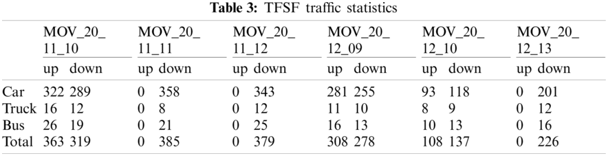
Using manual counting to get the accurate traffic flow of the test video, after several experiments to verify that the algorithm in this paper can still guarantee good accuracy and robustness, it can completely replace the inefficient work of manual counting. The accurate traffic flow results obtained after manual counting are as follows.

Error is used to evaluate the Error rate of TFSF, that is Error between the real traffic and the framework statistical traffic. Its calculation formula is as follows:

where i represents the type of vehicle detected, j represents the direction of movement of the vehicle, test_numi,j denotes the traffic statistics results of i vehicle j movement direction in the test video of the framework built in this paper, and real_numi,j denotes the real traffic results of i vehicle j movement direction.

From the comparative analysis in Tabs. 3–5, it can be seen that the traffic count error rate of the framework for Car is significantly lower than the other two, where the main reason is the large sample size, the number of labels in training set for Car is 9836, while the number of labels for Truck and Bus is 313 and 452, respectively, and the network model can be adequately trained. In addition, the scenes represented by the videos MOV_20_12_10 and MOV_20_12_10 are scenes of rainy day and night, respectively. The error rate of this scene is significantly higher than that of the scenes of a sunny day. The error rate of the scene of a rainy day is 12.2%, while that of the night is 18.7%. Therefore, the following research is mainly aimed at this particular scene, and various methods are adopted to improve the accuracy of this framework in the particular scene.

The average accuracy was used to evaluate the overall accuracy of TFSF. After calculation, the average accuracy is 93.6.

The framework is based on the traffic scene, accuracy is not the only evaluation standard, the framework of the speed of the framework is an important parameter, tested, the building of traffic statistics framework 32.7 FPS, fully meet the requirements of the real-time, after tests verify that the frame of video under various scenarios also has good robustness, can maintain a certain accuracy.

Compared with the existing traffic statistics system [23], the framework built in this paper uses better detection and tracking performance and distinguishes the direction of traffic flow and the type of vehicles. The test results show that the framework has high robustness under different scenarios.

This paper builds a traffic statistics framework based on detection and tracking, which is suitable for most traffic scenes. In order to consider the accuracy and speed of the framework detection, the YOLO V5s network structure was adopted. At the same time, the DeepSort tracking algorithm is improved to improve the performance of the algorithm. The framework can be divided into different vehicle types and movement directions to more detailed statistics of traffic flow and facilitate the integration of more functions, with an overall accuracy of more than 93%.

In the future research direction, the problem of decreased accuracy of traffic statistics caused by scene changes should be further solved. It is believed that the framework can provide some meaningful information for traffic decision-makers to improve the current traffic problems.

Funding Statement: This work is supported by the Qingdao People's Livelihood Science and Technology Plan (Grant 19–6–1-88-nsh).

Conflicts of Interest: The authors declare that they have no conflicts of interest to report regarding the present study.

References

1. Duan, M., (2018). Management system project design of urban intelligent transportation. Journal of Interdisciplinary Mathematics, 21(5), 1175–1179. DOI 10.1080/09720502.2018.1494585. [Google Scholar] [CrossRef]

2. Zhu, F. H., Lv, Y. S., Chen, Y. Y., Wang, X., Xiong, G. et al. (2020). Parallel transportation systems: Toward IoT-enabled smart urban traffic control and management. IEEE Transactions on Intelligent Transportation Systems, 21(10), 4063–4071. DOI 10.1109/TITS.6979. [Google Scholar] [CrossRef]

3. Aloimonos, Y., Rosenfeld, A. (1991). Computer vision. Science, 253(5025), 1249–54. DOI 10.1126/science.1891713. [Google Scholar] [CrossRef]

4. Lu, L. P., Li, H. S., Ding, Z., Guo, Q. M. (2020). An improved target detection method based on multiscale features fusion. Microwave and Optical Technology Letters, 62(9), 3051–3059. DOI 10.1002/mop.32409. [Google Scholar] [CrossRef]

5. Yi, X., Wang, B. J. (2017). Fast infrared and Dim target detection algorithm based on multi-feature. Acta Photonica Sinica, 46(6), 610002. DOI 10.3788/gzxb20174606.0610002. [Google Scholar] [CrossRef]

6. Li, S. W., Gu, X. Y., Xu, X. R., Xu, D. W., Zhang, T. J. et al. (2021). Detection of concealed cracks from ground penetrating radar images based on deep learning algorithm. Construction and Building Materials, 2021, 273–121949. DOI 10.1016/j.conbuildmat.2020.121949. [Google Scholar] [CrossRef]

7. Kakuda, K., Enomoto, T., Miura, S. (2019). Nonlinear activation functions in CNN based on fluid dynamics and Its applications. Computer Modeling in Engineering & Sciences, 118(1), 1–14. DOI 10.31614/cmes.2019.04676. [Google Scholar] [CrossRef]

8. Deng, X., Shao, H. J., Shi, L., Wang, X., Xie, T. L. (2020). A classification-detection approach of COVID-19 based on chest X-ray and CT by using keras pre-trained deep learning models. Computer Modeling in Engineering & Sciences, 125(2), 579–596. DOI 10.32604/cmes.2020.011920. [Google Scholar] [CrossRef]

9. Ren, P. M., Wang, L., Fang, W., Song, S. L., Djahel, S. (2020). A novel squeeze YOLO-based real-time people counting approach. International Journal of Bio-Inspired Computation, 16(2), 94–101. DOI 10.1504/IJBIC.2020.109674. [Google Scholar] [CrossRef]

10. Girshick, R., Donahue, J., Darrell, T., Malik, J. (2014). Rich feature hierarchies for accurate object detection and semantic segmentation. 2014 IEEE Conference on Computer Vision and Pattern Recognition (CVPRpp. 580–587. Columbus. DOI 10.1109/CVPR.2014.81. [Google Scholar] [CrossRef]

11. Girshick, R. (2015). Fast R-CNN. 2015 IEEE International Conference on Computer Vision (ICCVpp. 1440–1448. Santiago. DOI 10.1109/ICCV.2015.169. [Google Scholar] [CrossRef]

12. Liu, W., Anguelov, D., Erhan, D., Szegedy, C., Reed, S. et al. (2016). SSD: Single shot multiBox detector. European Conference on Computer Vision, pp. 21–37. Springer, Cham. DOI 10.1007/978-3-319-46448-0. [Google Scholar] [CrossRef]

13. Zeng, Q. L., Wen, G. J., Li, D. D. (2016). Multi-target tracking by detection. Proceedings of 2016 International Conference on Audio, Language and Image Processing (ICALIPpp. 370–374. USA. [Google Scholar]

14. Mekonnen, A. A., Lerasle, F. (2019). Comparative evaluations of selected tracking-by-detection approaches. IEEE Transactions on Circuits and Systems for Video Technology, 29(4), 996–1010. DOI 10.1109/TCSVT.76. [Google Scholar] [CrossRef]

15. Wojke, N., Bewley, A., Paulus, D. (2017). Simple online and realtime tracking with a deep association metric. 2017 24th IEEE International Conference on Image Processing (ICIPpp. 3645–3649. Beijing, China. [Google Scholar]

16. Li, Q., Li, R. Y., Ji, K. F., Dai, W. (2015). KF and its application. 2015 8th International Conference on Intelligent Networks and Intelligent Systems (ICINISpp. 74–77. Tianjin, China. [Google Scholar]

17. Gui, H. C., de Ruiter, A. H. J. (2018). Quaternion invariant extended KFing for spacecraft attitude estimation. Journal of Guidance Control and Dynamics, 41(4), 863–878. DOI 10.2514/1.G003177. [Google Scholar] [CrossRef]

18. Guo, S. J., Liu, F., Yuan, X. H., Zou, C. R., Chen, L. (2021). HSPOG: An optimized target recognition method based on histogram of spatial pyramid oriented gradients. Tsinghua Science and Technology, 26(4), 475–483. DOI 10.1109/TST.5971803. [Google Scholar] [CrossRef]

19. Wu, L., Ma, J., Zhao, Y. H., Liu, H. (2021). Apple detection in complex scene using the improved YOLOv4 model. Agronomy-Basel, 11(3), 176. DOI 10.3390/agronomy11030476. [Google Scholar] [CrossRef]

20. Wang, W. (2003). Scheme design technique of urban traffic management planning. Journal of Triffic and Transportation Engineering, 3(2), 57–60. DOI 10.3321/j.issn:1671-1637.2003.02.013. [Google Scholar] [CrossRef]

21. Li, T. F., Zou, Y., Bai, P. F., Li, S. X., Wang, H. W. et al. (2021). Detecting cerebral microbleeds via deep learning with features enhancement by reusing ground truth. Computer Methods and Programs in Biomedicine, 204, 106051. DOI 10.1016/j.cmpb.2021.106051. [Google Scholar] [CrossRef]

22. Chen, L., Ai, H. Z., Chen, R., Zhuang, Z. J. (2019). Aggregate tracklet appearance features for multi-object tracking. IEEE Signal Processing Letters, 26(11), 1613–1617. DOI 10.1109/LSP.97. [Google Scholar] [CrossRef]

23. Chen, Q. Q., Huang, N., Zhou, J. M., Tan, Z. (2018). An SSD algorithm based on vehicle counting method. 2018 37th Chinese Control Conference (CCC), pp. 7673–7677. Wuhan, China. DOI 10.23919/ChiCC.2018.8483037. [Google Scholar] [CrossRef]