Computer Modeling in Engineering & Sciences

DOI: 10.32604/cmes.2021.017321

ARTICLE

A GPU-Based Parallel Algorithm for 2D Large Deformation Contact Problems Using the Finite Particle Method

Wei Wang1,2, Yanfeng Zheng1,3, Jingzhe Tang1, Chao Yang1 and Yaozhi Luo*,1,*

1College of Civil Engineering and Architecture, Zhejiang University, Hangzhou, 310058, China
2Center for Balance Architecture, Zhejiang University, Hangzhou, 310028, China
3Architectural Design and Research Institute of Zhejiang University Co., Ltd., Hangzhou, 310028, China
*Corresponding Author: Yaozhi Luo. Email: luoyz@zju.edu.cn
Received: 01 May 2021; Accepted: 26 July 2021

1  Introduction

The numerical simulation of large deformation contact problems plays an important role in engineering fields. These problems generally involve geometric nonlinearity, material nonlinearity, and contact nonlinearity. Several numerical methods are available for these problems, among which the finite element method (FEM) is one of the most widely used methods. Computational contact mechanics using the FEM has been developed by many scholars since the 1970s and can be found in the literature [1,2]. Recently, some elaborated contact algorithms in the FEM context, such as the mortar method [3] and the surface smoothing method [4], have been developed, mainly to improve the accuracy of contact constraints; the computational efficiency of these algorithms, however, has drawn less attention. In fact, contact algorithms generally account for a considerable proportion of the overall computational cost [5]. Specifically, according to Wriggers [1], the time complexities of contact search algorithms are generally of the order from O(N) to O(Nlog⁡N), where N denotes the number of contact nodes, which is unacceptable when millions of elements come into contact. In addition, the strong nonlinearities involved in large deformation contact problems may cause difficulties when using implicit techniques [4], while the time step sizes for these contact problems are usually very small when using explicit techniques [5], resulting in time-consuming calculation processes. Other methods, such as the discrete element method (DEM), are available for solving contact problems, but the DEM is more suitable for modeling contact in discrete particulate systems [6,7] and contact between rocks [8,9]. Therefore, a more efficient and stable method is strongly needed in large deformation contact problems.

The finite particle method (FPM) [10], derived from vector mechanics [11–13], is another feasible method for solving large deformation contact problems. In the FPM, a physical body is discretized into a number of particles and elements in space, and the motion path of each particle in time is modeled by a sequence of time steps, as illustrated in Fig. 1. The particles in the FPM are assumed to carry structural variables such as mass, velocity, and displacement. Within each time step, Newton's second law is adopted to formulate the motion of particles, and explicit time integration schemes are used to solve the equations of motion. In recent years, numerical methods based on vector mechanics have been successfully applied to various types of structural analyses, such as the analysis of shell structures [14], multiple body kinematic movements involving large displacements and rotations [15,16], progressive collapse simulations of structures [17], shape analysis of tensile structures [18], train-bridge interaction simulation [19], and fluid-solid interaction simulation [20].

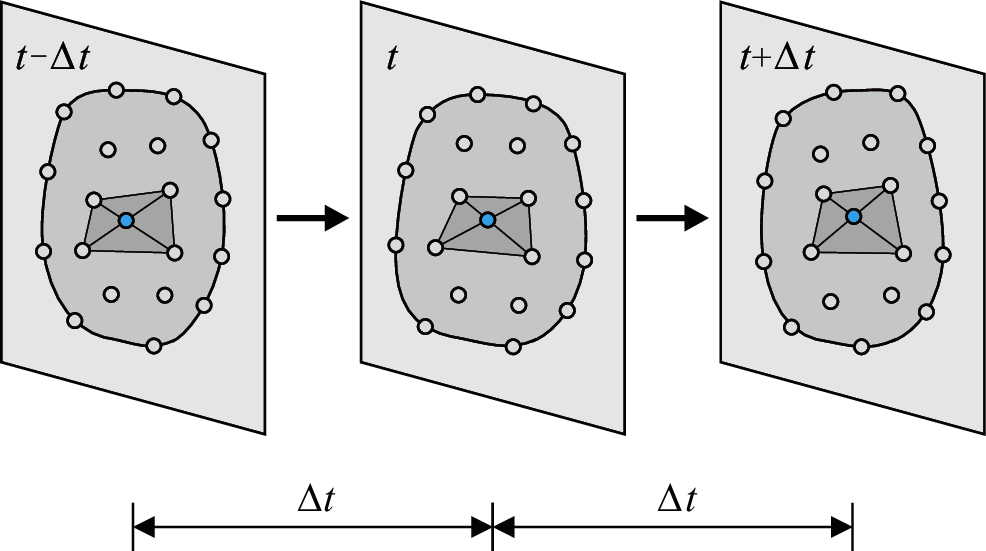
Figure 1: Discrete model of the FPM in space and time (only elements connected to the highlighted particle are depicted for brevity)

When dealing with large deformation problems, the FPM is effective in separating the pure deformation of elements from their total motion by using the fictitious reverse motion technique [10], which makes it suitable for solving large deformation contact problems. In addition, contact algorithms based on the explicit FEM, such as the one proposed by Hallquist et al. [21], can easily be adopted by the FPM due to the similar mechanisms of these two methods. However, contact calculation via the serially computed FPM is still time-consuming, mainly due to the small time step size for ensuring conditional stability of the method and the time-consuming contact search process. This problem can be effectively alleviated by using parallel acceleration for the FPM. In fact, no global stiffness matrix is assembled in the FPM, and the main solution procedures of the FPM are decoupled in nature; thus, the FPM is intrinsically suitable for parallel implementation with a high degree of parallelism.

Many parallel architectures are based on central processing unit (CPU) technology, e.g., open multiprocessing (OpenMP) [22,23] for multiple CPUs and message passing interface (MPI) for multiple computer hosts. However, the hardware costs of CPU-based parallel architectures are very high, and the quantitative restriction of CPU cores in personal computers makes concurrently processing a large number of procedures a difficult task. Recently, thanks to the development of graphics processing units (GPUs) with unified architectures and the introduction of specialized programming models, such as Compute Unified Device Architecture (CUDA) designed by NVIDIA, general-purpose computing on GPU (GPGPU) has become an increasingly adopted computing technique in engineering simulations [24–26]. While a CPU is designed to excel at executing a single thread as fast as possible, a GPU is designed to excel at executing thousands of threads in parallel [27]. As a result, GPUs provide higher instruction throughput and memory bandwidth at a lower cost than CPUs [28]. Therefore, the GPU architecture is more appropriate for parallel implementation of the FPM.

In this paper, a two-dimensional GPU-based parallel contact algorithm using the FPM is proposed and implemented based on the GPU-accelerated software developed in our previous study [24]. The algorithm takes full advantage of the parallel architecture of GPUs, and the main computational procedures of the algorithm, including evaluating elemental internal forces, searching contact pairs, detecting contact states, calculating contact forces, and solving the equations of motion, are executed in parallel on a GPU. There are four contributions of the current work compared to our previous study [24]: (1) two new quadrilateral elements FPM-Q4 and FPM-Q4R are developed for 2D large deformation problems; (2) a contact algorithm for 2D large deformation problems is proposed and incorporated into FPM; (3) The proposed contact algorithm is parallelized based on GPU; (4) the parallel contact algorithm is verified and its performance is fully tested.

This paper is structured as follows. The fundamentals of the parallelized FPM for planar solids are briefly introduced in Section 2. The parallel contact algorithm is discussed in Section 3, including the contact detection process and calculation of the contact forces. The GPU implementation of the proposed algorithm is presented in Section 4. Two verification examples and two performance tests are presented in Section 5 to demonstrate the accuracy and efficiency of the proposed contact algorithm. Finally, conclusions are given in Section 6.

2  Fundamentals of the Parallelized FPM for Planar Solids

The fundamentals of the FPM for planar solids are briefly described in this section, including the equations of motion of particles and the internal forces of quadrilateral elements. Readers are referred to the literature [12] for more details. The parallel algorithm for planar solids is presented in Section 2.3.

2.1 Equations of Motion of Particles

A planar solid, as shown in Fig. 2a, can be discretized into 20 particles and 12 quadrilateral elements. For an arbitrary particle α, the equation of motion can be formulated based on Newton's second law:

mαd¨α=Fαext−Fαint−Fαdmp+Fαc(1)

where mα is the mass of particle α, d¨α represents the acceleration vector, Fαext denotes the external forces applied to particle α, Fαint represents the internal forces of particle α passed from the elements connected to it (see Section 2.2), Fαc denotes the contact forces (derived in Section 3.2), and Fαdmp represents the mass-proportional damping force, which is given by

Fαdmp=ξmαd˙α(2)

where ξ is the damping coefficient and d˙α denotes the velocity vector of particle α. The particle forces are illustrated in Fig. 2b.

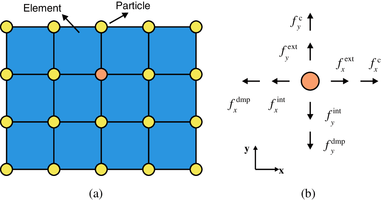
Figure 2: Discretization of a planar solid: (a) Particles and elements; (b) Particle forces

The central difference method is adopted to solve Eq. (1) because of its low computational cost and sufficient accuracy. According to the literature [29], the central difference method has the highest accuracy and maximum stability limit for any second-order accurate explicit method. Other explicit time integration algorithms such as generalized-α algorithm [30] can also be utilized in the FPM, but more computational time will be taken when using those algorithms. Thus, the central difference method is adopted in this paper to solve the equations of motion of particles. Given the particle displacements at times t−Δt and t, where Δt is the time step size, the particle displacement at time t+Δt can be explicitly expressed as follows:

t+Δtdα=c1Δt21mα(tFαext−tFαint+tFαc)+2c1tdα−c2t−Δtdα(3)

where c1=(1+ξΔt/2)−1 and c2=c1(1−ξΔt/2).

2.2 Internal Forces of Quadrilateral Elements

The internal forces of quadrilateral elements are derived in this section. First, the pure deformation is approximated by using fictitious reverse motion, and a local coordinate system (LCS) is introduced based on the pure deformation vector. Subsequently, the strain and stress increments are computed in the LCS, and the internal forces are derived using the principle of virtual work.

2.2.1 Pure Deformation

As shown in Fig. 3a, a quadrilateral element moves from time ta to tb, where tb=ta+Δt. The corresponding configurations are denoted as Ωa and Ωb, respectively, and the position vectors of each particle are represented as Xia and Xib(i=1,2,3,4), respectively. The incremental displacement vectors of the particles from time ta to tb are denoted as

Δdi=Xib−Xia,(i=1,2,3,4)(4)

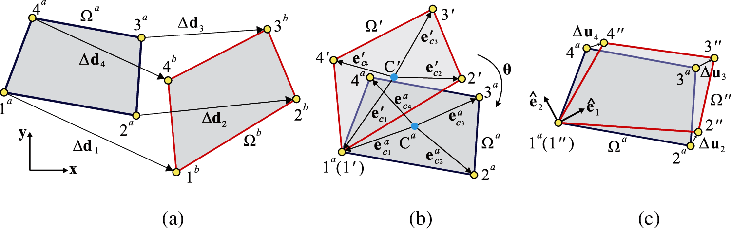
Figure 3: Fictitious reverse motion for calculating pure deformation: (a) Configurations Ωa and Ωb; (b) Fictitious configuration Ω′; (c) Fictitious configuration Ω′′ and the local coordinate system

To separate the rigid-body motion from the total displacement, a fictitious reverse motion technique based on vector mechanics [12] is adopted, and the procedures are described as follows:

Step 1: Fictitious reverse translation. In the following, particle 1 is chosen as a reference particle. The configuration Ωb is translated to a fictitious configuration Ω′, as shown in Fig. 3b, by a vector of −Δd1, and the corresponding position vector Xi′ is expressed as

Xi′=Xib−Δd1,(i=1,2,3,4)(5)

Step 2: Fictitious reverse rotation. The configuration Ω′ is rotated to another fictitious configuration Ω′′, as shown in Fig. 3c, where the rotation axis is orthogonal to the plane containing the elements, and the rotation angle is obtained by

θ=14∑i=14⁡asineci′×eciaeci′×ecia,(i=1,2,3,4)(6)

where ecia and eci′ are the unit vectors pointing from the centroid of the element to particle i based on configurations Ωa and Ω′, respectively. The position vector of the particles in configuration Ω′′ is obtained by

Xi′′=X1′+R1(Xi′−X1′),(i=1,2,3,4)(7)

where R1 is the matrix representing the rotation from Ω′ to Ω′′, which is calculated using Rodrigues’ rotation formula [31]:

R1=[cos⁡θ−sin⁡θsin⁡θcos⁡θ](8)

Step 3: Pure deformation approximation. Since the rigid motion is separated from the total displacement through the fictitious reverse motion, the pure deformation matrix of the element is approximated as

ΔU=[Δu1Δu2Δu3Δu4]T(9)

with

Δui=Xi′′−Xia,(i=1,2,3,4)(10)

Step 4: Definition of the LCS. An LCS with axes e^1, e^2, and e3, as shown in Fig. 3c, is introduced to reduce the total number of independent variables and simplify the process of internal force calculation; here, the unit vector e3 is orthogonal to the plane, e^1=[e^1x,e^1y] is parallel to Δui with the greatest magnitude (e.g., Δu3 in Fig. 3c), and e^2=[e^2x,e^2y]=e3×e^1. The corresponding pure deformation matrix in the LCS, denoted as ΔU^, is obtained by

ΔU^=R2ΔU(11)

where R2 is the transformation matrix from the global coordinate system (GCS) to the LCS:

R2=[e^1xe^1ye^2xe^2y](12)

2.2.2 Strain and Stress Increments

After obtaining the pure deformation, the concepts of shape function and isoparametric transformation developed in the conventional FEM are introduced to the FPM to describe the strain and stress distributions within each quadrilateral element. The strain increment vector at each integration point in the LCS is given as

Δε^i=B^iΔU^,(i=1,2,…,Nint)(13)

where Nint is the number of integration points and B^i denotes the strain-displacement matrix at the ith integration point in the LCS. The details of isoparametric transformation for quadrilateral elements are omitted here for brevity but can be found in the literature [32].

The stress increment vector at each integration point in the LCS can be evaluated as

Δσ^i=DeΔε^i,or Δσ^i=DepΔε^i(i=1,2,…,Nint)(14)

where De and Dep denote the elastic and elastoplastic constitutive matrices, respectively. For plastic materials, the combined isotropic-kinematic hardening is utilized in the FPM based on the J2 flow theory [33]. The yield function is

f(σ,α,κ)=‖ξ‖−κ≤0,ξ=s−α

where σ is a Cauchy stress tensor, s is a deviatoric stress tensor, α is a deviatoric back stress tensor, ξ is called the effective stress, and κ is the plastic internal variable. The radial return algorithm for J2 theory is adopted to determine the actual form of Dep in Eq. (14), which can be found in the literature [34].

2.2.3 Internal Forces

The principle of virtual work is adopted to derive the internal forces of elements. For each element, the variation of the external work, δUext, done by the elemental internal force F^e is

δUext=(δΔU^)TF^e(15)

and the variation of the internal work, δUint, done by the element stress σ^ is

δUint=∫V⁡(δΔε^)Tσ^dV=(δΔU^)T∫V⁡B^Tσ^dV(16)

Considering that δUext=δUint, the elemental internal force in the LCS can be evaluated as

F^e=∫V⁡B^Tσ^dV(17)

Note that the internal forces of elements in the LCS should be transformed back to the GCS by

Fe=R2−1R1−1F^e(18)

The equivalent internal force of particle α is a sum of the internal forces of the elements connected to it, i.e.,

Fαint=∑i=1n⁡Fie(19)

where n denotes the number of elements connected to particle α.

2.2.4 Integration Schemes

Two integration schemes of elemental internal forces are adopted in this paper. The first one is the selective integration technique (also called the B bar method) proposed by Hughes [35], which provides good accuracy for both compressible and nearly incompressible media by using a one­point integration for volumetric stresses and a two­point quadrature in each direction for the deviatoric stresses. The corresponding elements of the B bar method are called FPM-Q4 and used in Section 5.1. The other integration scheme is the uniform reduced integration with hourglass control developed by Flanagan et al. [36]. The corresponding elements with this reduced integration technique are called FPM-Q4R and used in Section 5.2.

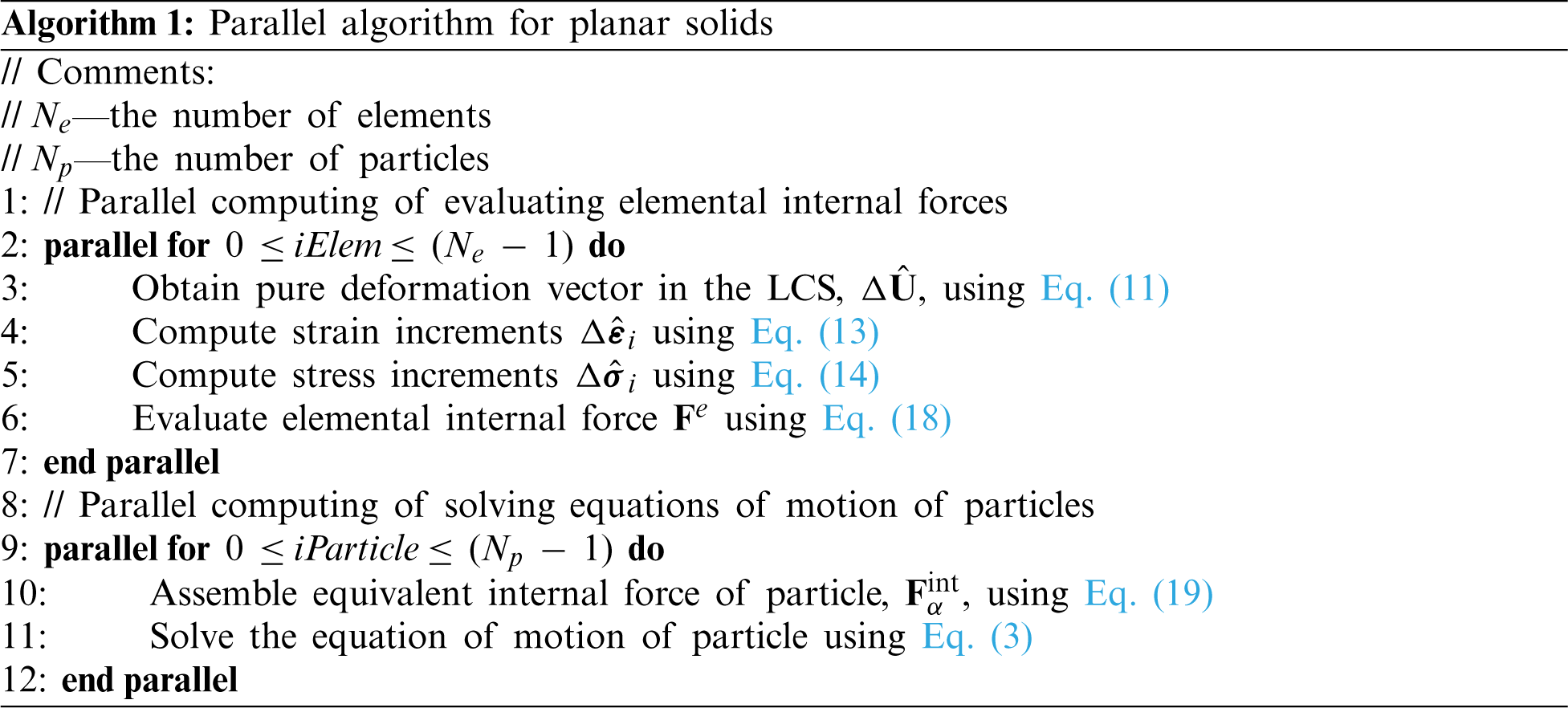
2.3 Parallel Algorithm for Planar Solids

The parallel algorithm for planar solids is presented in Algorithm 1. Note that the keyword pair “parallel for … end parallel” indicates that the codes within it are executed in parallel on GPU threads. The equation of motion of each particle is solved individually, and the evaluations of the elemental internal forces are self-reliant between elements; thus, the FPM can be accelerated by GPGPU techniques with a high degree of parallelism. The corresponding GPU implementation for planar solids is given in Section 4.

3  Parallel Contact Algorithm Based on the FPM

3.1 Contact Detection

The contact between two deformable bodies is considered. The contact surface on one body is selected as the master and the contact surface on the other body as the slave, as shown in Fig. 4, and this master-slave pair is called a contact surface pair. The node-to-segment (NTS) [21] technique is adopted for discretizing contact surfaces into contact particles and contact segments, as shown in Fig. 4. After discretizing contact bodies, the particles on the master surface are defined as master particles while the particles on the slave surfaces as slave particles. Note that proper selection of the master and slave surfaces is significant for NTS contact discretization. According to the literature [4], the selection of master and slave surfaces should satisfy that the slave nodes cannot penetrate into the master surface, while the master nodes are free to penetrate into the slave surface. Thus, the contact surface of the stiffer body should be the master surface. More details about choosing the master and slave surfaces can be found in the literature [4].

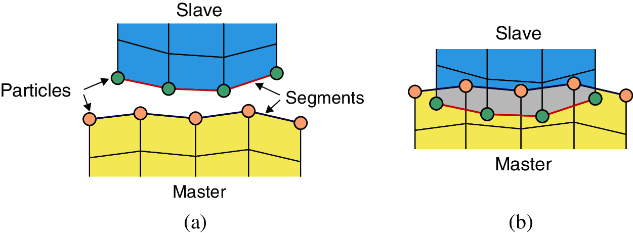
Figure 4: Discretization of contact surfaces: (a) Separation state; (b) Penetration state

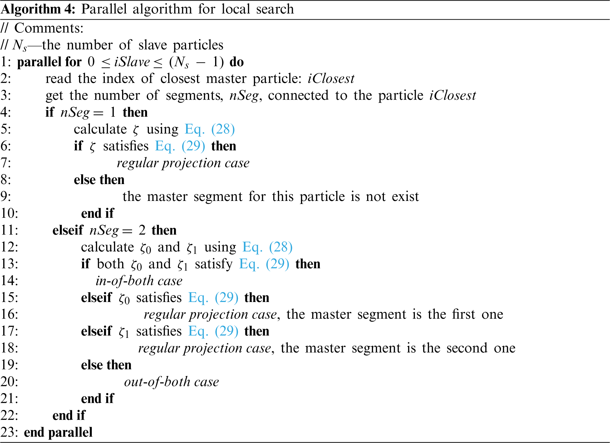
The contact search algorithms of contact surfaces are typically decomposed into two distinct phases: global search and local search. The purpose of global search is to first collect master segment candidates for each slave particle, and the aim of local search is to choose the exact master segment for each slave particle and detect the contact state. Note that global search can be performed every n time steps to reduce the computational time, while local search needs to be performed at every time step. To make this contact search algorithm more suitable for parallel computing, a linked-list data structure represented by two arrays [37] is used.

3.1.1 Data Structure

For a two-body contact problem, the potential range of a contact surface pair in space is represented by a bounding box, as illustrated in Fig. 5. The coordinates of the bottom-left and top-right corners of the bounding box are denoted as (xmin,ymin) and (xmax,ymax), respectively. The bounding box is divided into several square cells of the same size, and the size of each cell is determined by

Lc=λL¯(20)

where L¯ is the average length of all contact segments, λ is a cell size scale factor with a default value of 1.0. The number of cells in each direction is obtained by

Nx=floor(xmax−xminLc)+1(21)

Ny=floor(ymax−yminLc)+1(22)

where floor(⋅) is an operator used to round a number downwards to the nearest integer. The total number of cells is calculated by

Nc=NxNy(23)

Subsequently, each particle of the contact surface pair can be mapped into a cell, and the cell index is calculated by

ic=ix+iyNx(24)

where ix=floor((x−xmin)/Lc) and iy=floor((y−ymin)/Lc) are indices of the cell along the x and y directions, respectively, and (x,y) is the coordinate of the particle.

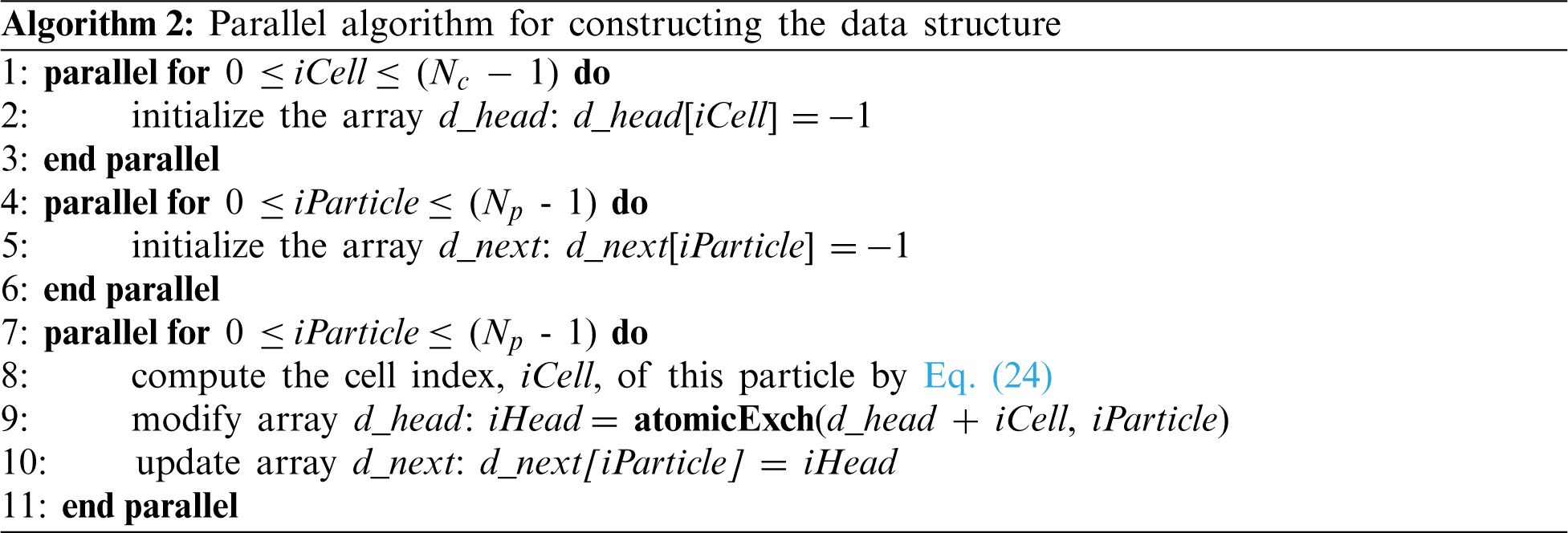
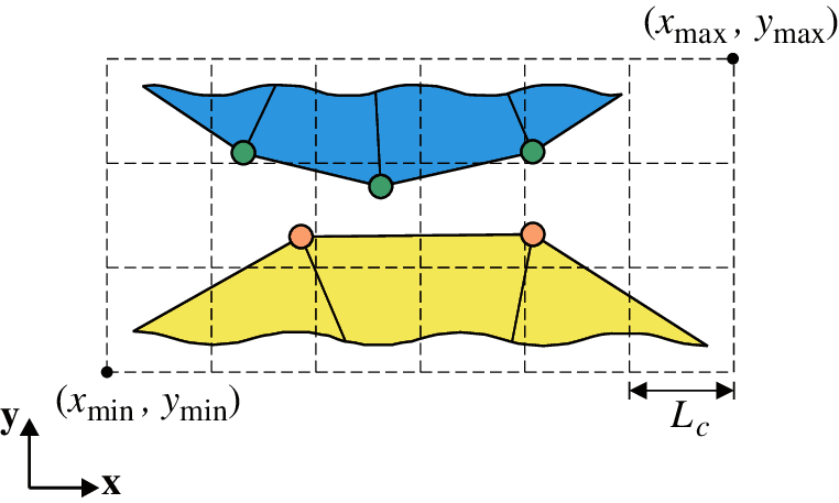
Figure 5: Space decomposition of the bounding box of a contact surface pair

A linked-list data structure [37] is adopted to store the particles in each cell. This data structure is beneficial to the parallel global search process and suitable for the coalescence access of GPU memory. A bounding box that is divided into 16 cells is taken as an example, as shown in Fig. 6, with 20 contact particles located within these cells. Two arrays are used to construct the linked list, as illustrated in Fig. 7a. The array d_head is used to store the first contact particle index in each cell, and the array d_next is used to link the remaining particle indices in the same cell [38]. Note that each element in array d_next indicates the index of the next particle until −1 is encountered. For example, particles 10, 8, and 7 are located in the 6th cell (ix= 2, iy= 1); therefore, particle 10 is stored in the 6th element of array d_head, while particles 8 and 7 are stored in the 10th and 8th elements of array d_next, respectively, and the 7th element of array d_next is set to −1 to indicate the end of the linked list. The lengths of these two arrays are Nc and Np, respectively, where Np denotes the number of contact particles.

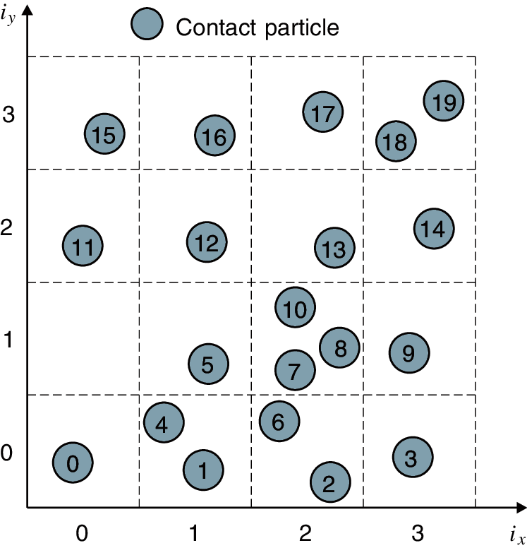
Figure 6: Mapping of contact particles into cells

The main steps for constructing the data structure for a contact surface pair are described in Algorithm 2. The elements of arrays d_head and d_next are initialized to −1. The indices of particles located in the same cell are stored in the linked list one by one. Note that the function b = atomicExch(addr, a) is an atomic function in the CUDA toolkit to replace the value at the address addr with value a and then return the old value b, which performs a read-modify-write atomic operation in a thread and guarantees no interference with other threads [27]. For multiple surface pairs, the contact particles of all pairs can be stored in a single linked-list data structure, as shown in Fig. 7b. This data structure ensures the efficiency of parallel contact search for contact problems with multiple surface pairs, which is validated in Section 5.2.

Figure 7: Linked-list data structure: (a) One surface pair; (b) Multiple surface pairs

3.1.2 Parallel Global Search

The global search consists of two steps: (1) find the closest master particle for each slave particle and (2) choose the segments connected to this master particle as master segment candidates. The closest master particle can be identified by looping for all master particles, which is time-consuming. To improve the efficiency, only particles located in the nine (3 × 3) neighboring cells are detected in this study [39]. The loop of the particles in each cell takes advantage of the well-organized data structure built above. Note that this approach will miss some segment candidates if the cell size is too small. As shown in Fig. 8, if the two particles of a segment are located outside of the nine cells, this segment cannot be detected. Therefore, the cell size should satisfy the following condition:

Lc≥Lmax/3(25)

where Lmax is the maximum length of all master contact segments. The parallel global search procedures for each slave particle are summarized in Algorithm 3.

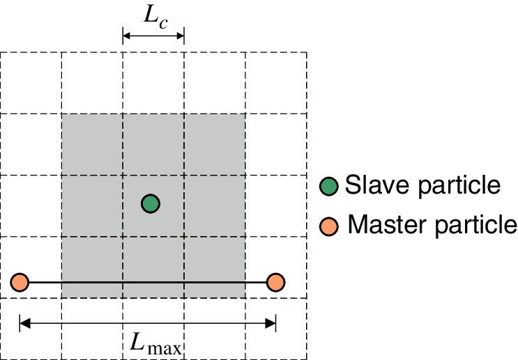
Figure 8: Minimum cell size length requirement

3.1.3 Parallel Local Search

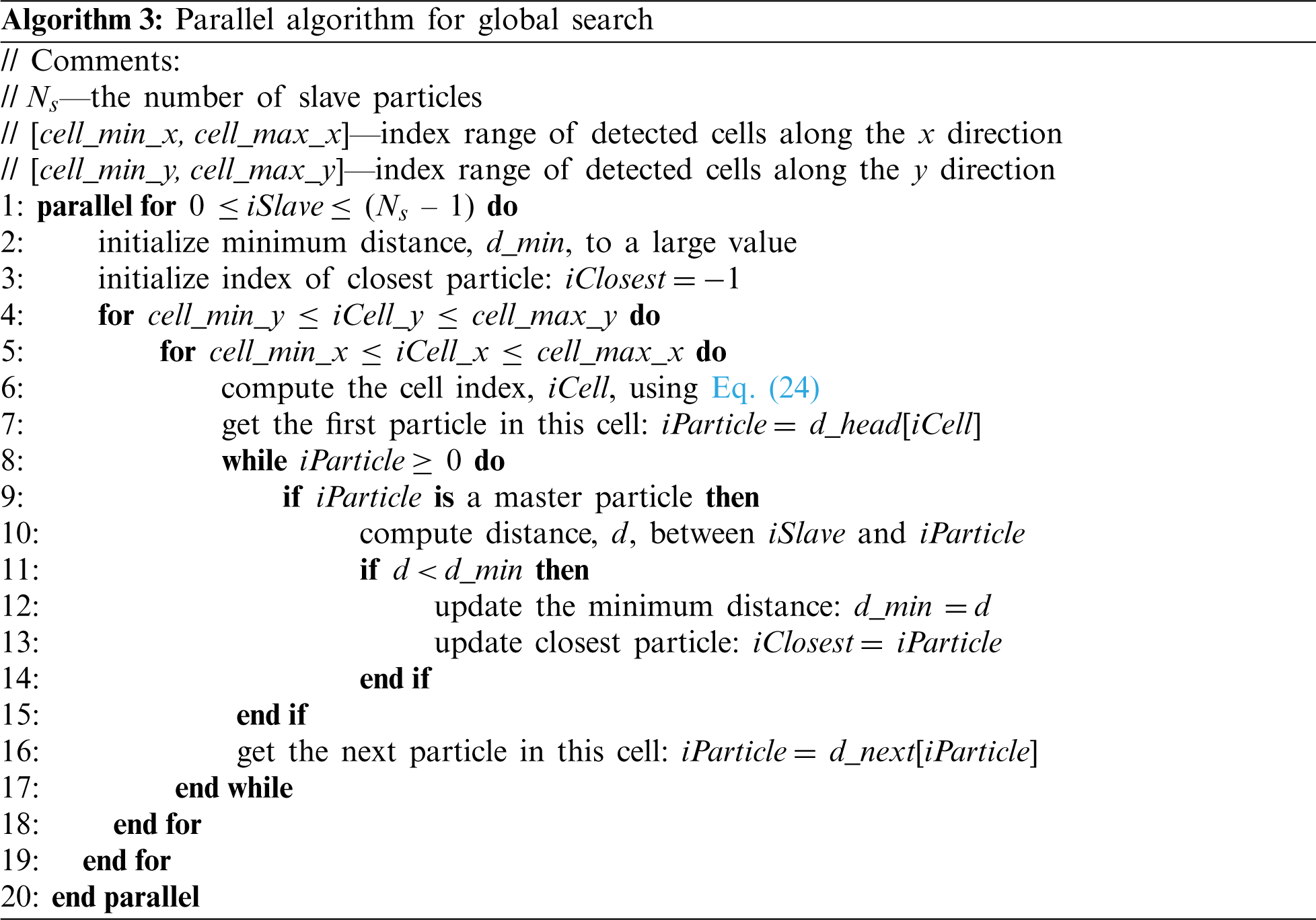
To choose the exact master segment, projections of the slave particle onto each segment candidate should be performed first. Fig. 9 illustrates the projection of a slave particle S onto a master segment candidate CM. Particle C is the closest master particle to particle S. The position vectors of these three particles are denoted by XS, XC, and XM, respectively.

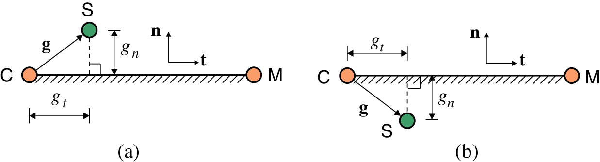
Figure 9: Projection of slave particle onto a master segment candidate: (a) Open gap (gn>0); (b) Closed gap (gn≤0)

An LCS with unit vectors t, n and e3 is introduced. The tangent vector t is parallel to the master segment

t=m‖m‖(26)

where m=XM−XC is the master segment vector, the vector e3 is orthogonal to the plane containing contact bodies, and the normal vector n=e3×t. The gap normal and tangential projections, gn and gt, are determined by

gn=g⋅n,gt=g⋅t(27)

where g=XS−XC is the gap vector. In addition, a normalized gap tangential projection, ζ, is introduced by

ζ=gt‖m‖(28)

and the range of ζ is

−ζtol≤ζ≤1+ζtol(29)

where ζtol is a tolerance that can be set to 1/50 [40].

Generally, three projection cases exist, as illustrated in Fig. 10, i.e., a regular case and two special cases: the “in-of-both” case and “out-of-both” case. For the regular case shown in Fig. 10a, gn is calculated by Eq. (27). For the other two special cases shown in Figs. 10b and 10c, the contact between the slave particle and its master segments is simplified to the contact between the slave particle and its closest master particle. Note that more accurate treatments for these two special cases can be found in the literature [40].

Figure 10: Projection cases: (a) Regular case; (b) “In-of-both” case; (c) “Out-of-both” case

Once the master segment has been identified, the gap status (open or closed) can be determined by checking the sign of gn, as shown in Fig. 9. An open gap indicates that the contact surfaces are separated with no need to enforce contact constraints, while a closed gap indicates that the contact forces should be calculated and exerted on the contact particles, which is discussed in Section 3.2. The parallel local search procedures for each slave particle are summarized in Algorithm 4.

3.2 Contact Forces

The penalty method is adopted to calculate the contact forces of particles due to its simplicity and ease of implementation. The calculations of the normal contact force and tangential contact force (i.e., friction force) using the penalty method are discussed in Sections 3.2.1 and 3.2.2, respectively. Note that the contact forces are calculated in parallel for each slave particle, and then the reaction forces are applied in parallel to the corresponding master particles.

3.2.1 Normal Contact Force

The magnitude of the normal contact force calculated by the penalty method is proportional to the amount of penetration, as shown in Fig. 11. For a contact pair composed of slave particle S and master segment CM, assuming that its projection case is regular (see Fig. 10a), the normal contact force is determined by

Fn=ϵn|gn|⋅n(30)

where ϵn is the normal penalty parameter of the master segment CM, gn is the normal gap, and n is the normal unit vector of CM. The penalty parameter is obtained using the following equation proposed by Hallquist et al. [5,21]:

ϵn=snKA2V(31)

where K is the bulk modulus of segment CM, A is the area of the segment, V is the volume of the element that contains segment CM, sn is a scale factor to adjust the normal penalty parameter. Note that appropriate penalty parameters are important for contact force calculation, because too large penalty parameter leads to non-convergent results, while too small penalty parameter results in unrealistic large penetration. In this paper, the scale factor sn is initially set to default value of 1.0 and then adjusted via a trial-and-error process until a satisfying result is obtained.

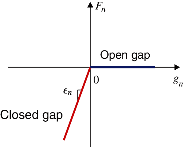
Figure 11: The relation between the normal contact force and normal gap

For the other two special projection cases, as shown in Figs. 10b and 10c, ϵn in Eq. (30) is set to the average value of the penalty parameters of segments CM1 and CM2. This approach is used to consider the contact stiffness contributions of both segments and reduce the variation of contact stiffness when the slave particle slides from one master segment to the other.

3.2.2 Friction Force

The most commonly used friction model is the classic Coulomb friction model [41]. However, the friction force of the Coulomb model is discontinuous at zero velocity, which may lead to oscillation results. A smoothed friction model [5] is adopted in this study. The friction force calculation is an adaptation of the radial return algorithm for elastic-perfectly plastic materials and can be described as follows:

Let tFn represent the normal contact force of slave particle S at time t calculated by Eq. (30), μ denote the coefficient of friction, and t−ΔtFs represent the friction force at time t−Δt. Then, the friction force at time t is calculated by the following steps:

1.    Compute the magnitude of the maximum static friction force:

tFs,max=μ‖tFn‖(32)

(2)   Calculate the trial friction force:

tFs∗=t−ΔtFs−ϵt(tdr−t−Δtdr)(33)

where t−Δtdr and tdr denote the relative displacements between slave particle S and master segment CM at times t−Δt and t, respectively; ϵt is the tangential penalty parameter of master segment CM, which is determined by:

ϵt=stKA2V(34)

where st is a scale factor with a defau value of 1.0 and is used to adjust this penalty parameter.

(3)   If the trial force does not exceed the maximum friction force, the friction is identified as static, and the friction force at time t is equal to thitrial force; otherwise, the friction is identified as kinetic, and the magnitude of the friction force at time t should equal tFs,max.

tFs={tFs∗if‖tFs∗‖≤tFs,maxtFs,maxtFs∗‖tFs∗‖if‖tFs∗‖>tFs,max(35)

Note that the friction force is considered only in the regular projection case (see Fig. 10a).

Once the normal and tangential contact forces of slave particle S have been obtained, the resultant contact force, as shown in Eq. (1), is cculated by

FSc=Fn+Fs(36)

As shown in Fig. 12a, the reaction contact forces applied to the particles of the master segment CM in the regular case can be calculated by

FCc=−(1−ζ)FSc,FMc=−ζFSc(37)

In the other two special projection cases, the reaction force applied to the closest master particle C has the same magnitude but opposite direction compared to FSc, as shown in Figs. 12b and 12c.

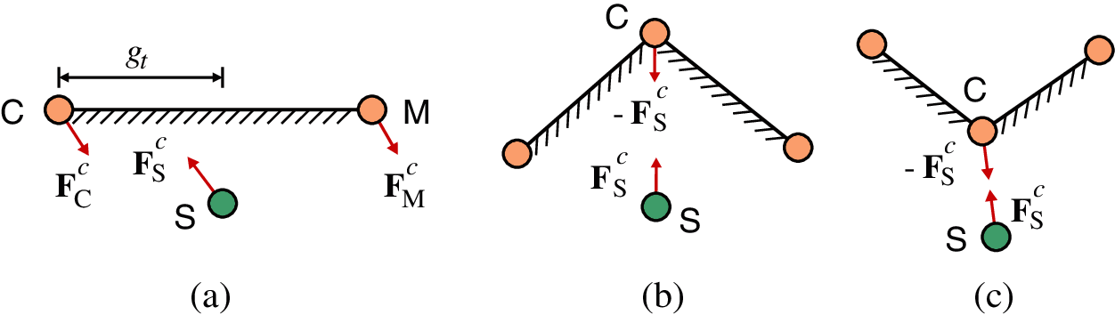
Figure 12: Reaction contact force of master particles: (a) Regular case; (b) “In-of-both” case; (c) “Out-of-both” case

4  GPU Implementation

The proposed contact algorithm based on the FPM is suitable for parallel implementation, as described in Sections 2 and 3. The GPU architecture is more appropriate than the CPU architecture for the parallel implementation of the FPM, as mentioned in Section 1. The parallel contact algorithm is implemented in the GPU-accelerated software developed in our previous study [24]. The algorithm is executed on NVIDIA GPUs powered by CUDA. The CUDA programming model is briefly introduced in Section 4.1, and the GPU implementation of the algorithm is presented in Section 4.2.

4.1 CUDA Programming Model

A generic CUDA application mainly consists of two parts: host code, running serially on a CPU, and device code, running in parallel on a GPU, as illustrated in Fig. 13. The host code is responsible for organizing host and device memories and managing the transfer of data between them. The device code consists of several device functions, named kernels, that are executed on GPU threads. The threads are organized into n-dimensional blocks, which are then organized into an n-dimensional grid (where n can be 1, 2, or 3), as depicted in Fig. 13. For a more detailed description of the CUDA programming model, the reader is referred to the literature [27].

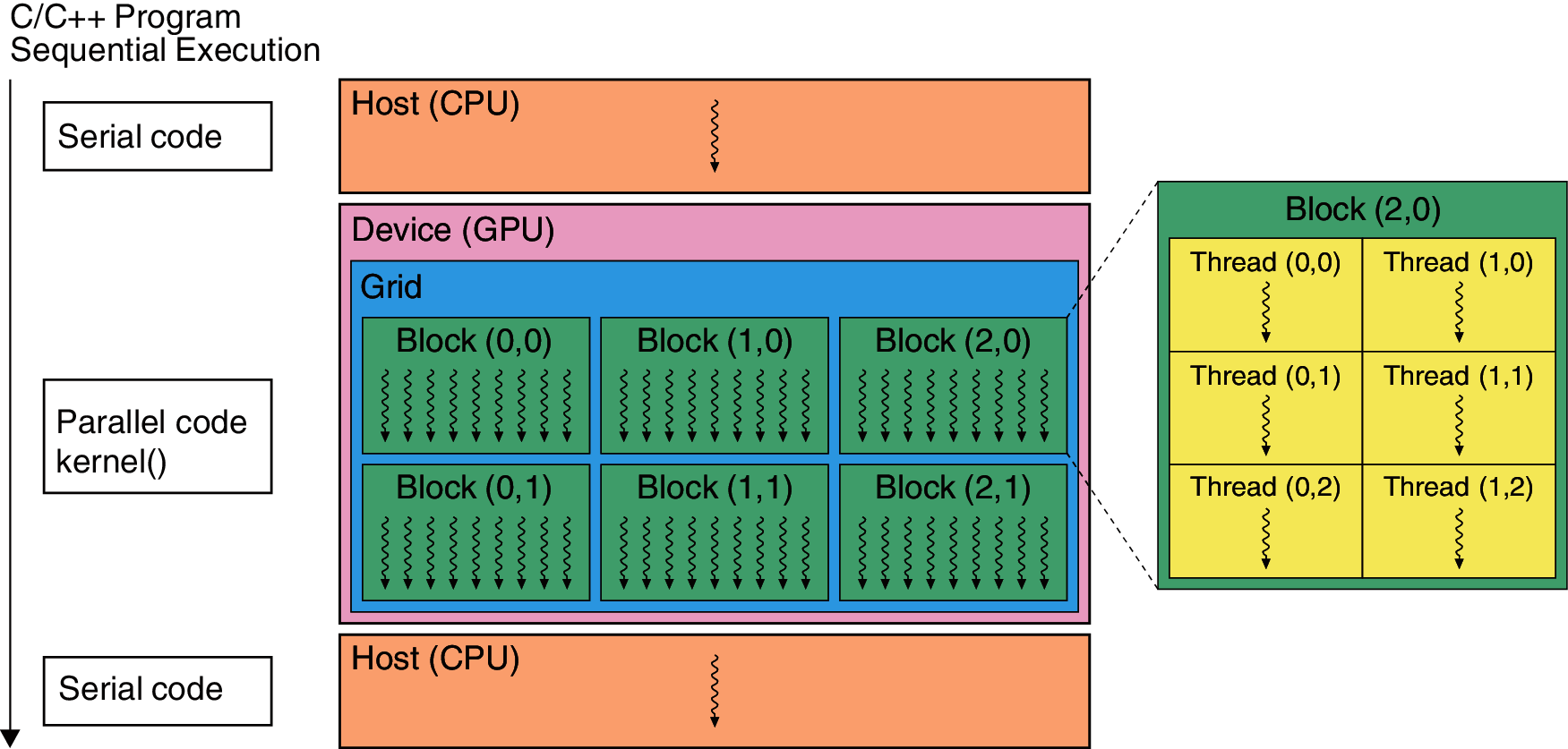
Figure 13: Schematic illustration of the CUDA programming model

4.2 GPU Implementation of the Algorithm

The flowchart of the parallel contact algorithm implemented in the FPM software is presented in Fig. 14. After preprocessing, the model data and variables are organized in the host memory and transferred to the device memory. A sequence of time steps is then performed for the analysis. Within each time step, the computational procedures are executed in a series of CUDA kernels managed by three FPM solvers: element solver, contact solver, and particle solver. Typically, the solution procedures consist of four main steps:

(1)   Element solver: evaluate the elemental internal forces in parallel for each element, as described in Section 2.2.

(2)   Contact solver:

(3)   Particle solver: solve the equation of motion in parallel for each particle using Eq. (3).

(4)   Time step controller: if the current time step is the last one, stop the calculation; otherwise, go to Step (1) and start the iteration for the next time step.

As described in our previous study [24], memory management is important to achieve satisfactory performance of the FPM solvers. Among all memory spaces available in CUDA, global device memory is the most widely used for all FPM solvers because it has the largest storage capacity. The global memory can be accessed by all threads using aligned memory transactions. The optimization of global memory throughput can be achieved if the memory access patterns are suitable for coalescence [25], which requires adjacent threads to access successive memory addresses. To achieve this coalescence of memory accesses, an adaptation of the structure-of-arrays (SoA) storage pattern [42] is adopted to manage all data buffers in global memory. In addition to memory management, the thread block size impacts the kernel performance. Based on performance tests for most of the kernels implemented in this study, 128 threads per block results in the best efficiency; thus, for convenience, the thread block size is set to a constant value of 128 for all kernels.

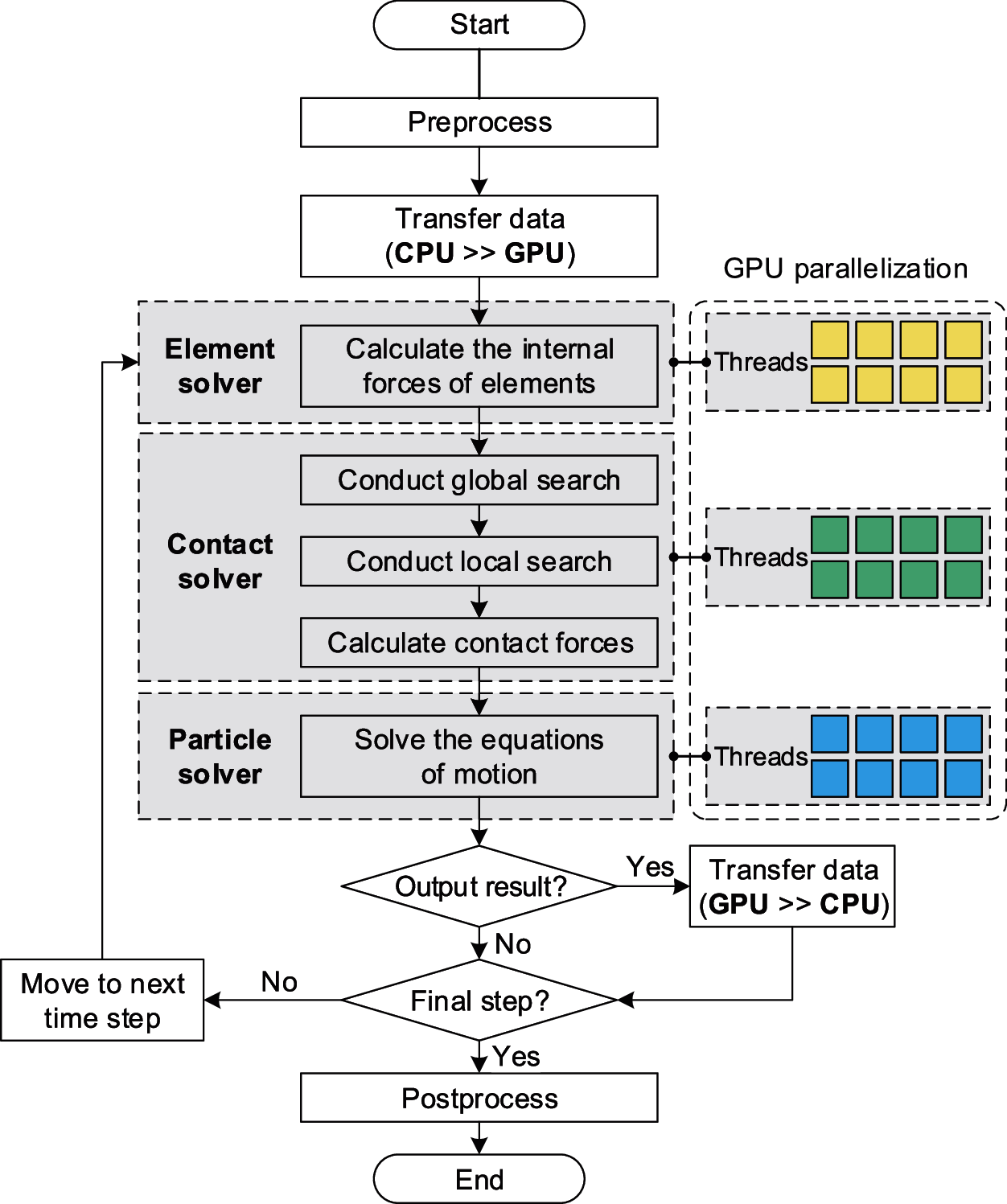
Figure 14: Flowchart of the GPU-based parallel contact algorithm

5  Numerical Examples

The effectiveness of the proposed contact algorithm is verified by two examples as presented in Section 5.1. Subsequently, the performance of the algorithm is tested in Section 5.2. All examples are computed under the assumption of a plane strain condition with a unit thickness of 1.0.

5.1 Verification

In this section, two verification examples are presented to demonstrate the accuracy of the proposed contact algorithm. These two examples focus on the frictional contact between two deformable bodies undergoing large sliding and large deformation. The first example involves elastic behavior, while the second example involves elastoplastic behavior. Fictitious mass damping is used in the verification examples to obtain static solutions. The quadrilateral element FPM-Q4, as described in Section 2.2.4, is used for the analyses in this section.

5.1.1 Contact in Elastic Problem

This numerical example is the so-called frictional ironing problem, which was previously studied in the literature [4,43]. The example comprises the sliding of a deformable block along an elastic slab, as illustrated in Fig. 15. The slab is fixed at its bottom surface, whereas the block is subjected to an imposed displacement at its upper surface. There are two load steps. From 0 to 1 s, a downward displacement uy= −10 mm is applied to the block, while from 1 to 2 s, the block slides horizontally along the slab with a displacement ux= 250 mm. The material parameters are given in Fig. 15, and the mass damping coefficient is set to ξ = 1.0× 105. The friction coefficient between the contact surfaces is μ=0.3. The block and slab are discretized into 136 and 3,840 quadrilateral elements, respectively. The scale factors for the normal and tangential penalty parameters are set to sn= 20.0 and st= 0.7, respectively.

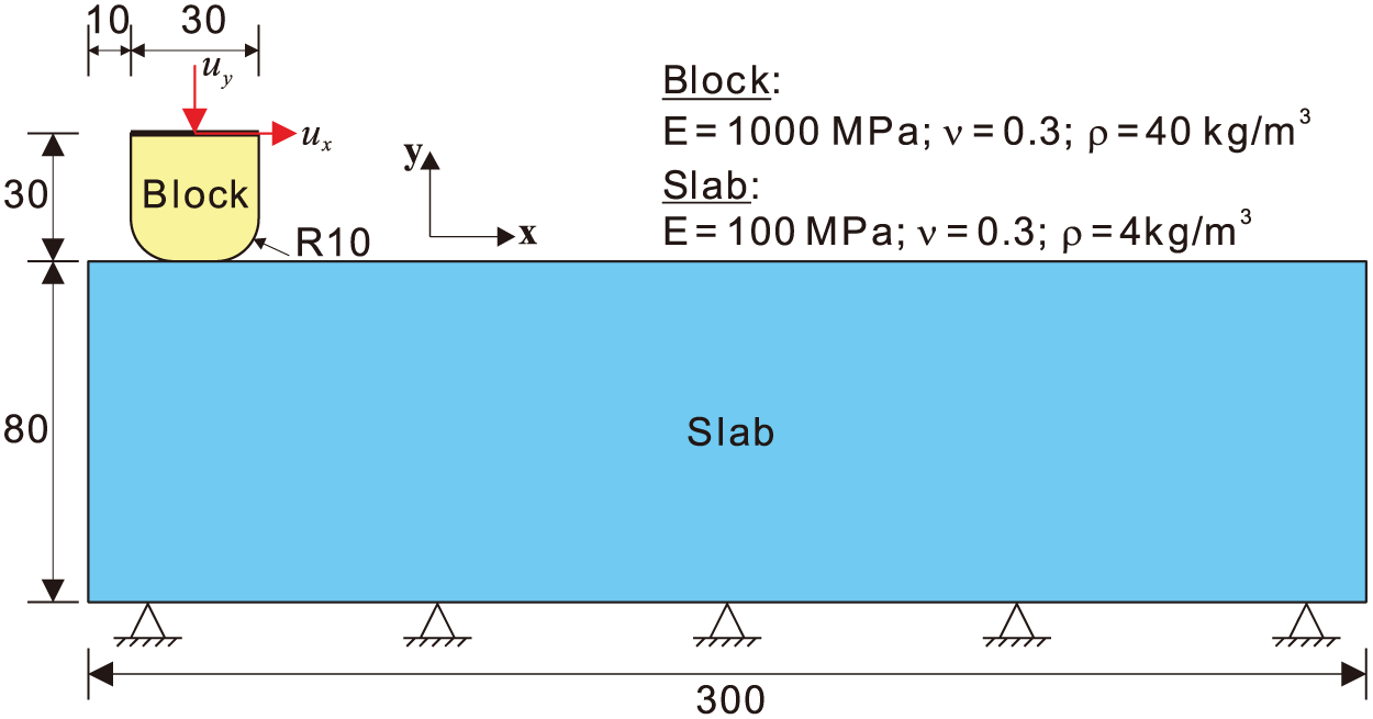
Figure 15: Geometry and material properties of the ironing problem (unit of length: mm)

The deformed configurations with a shear stress distribution are presented in Fig. 16 for three typical instants. In addition, the evolution of the total contact force components between the contacting bodies is presented in Fig. 17. From 0 to 1 s, as the vertical displacement of the block increases, the normal contact force gradually increases. The deformed configuration of the slab is not symmetrical; thus, the horizontal force component is not equal to zero. Starting from 1 s, the block begins to slide on the slab. The normal contact force increases slightly and remains constant afterwards. The horizontal force increases sharply after 1 s due to the contribution of the friction force and remains constant afterwards. Both contact force components drop slightly when the block reaches the right end of the slab. The results calculated by the FPM agree well with those obtained by Neto et al. using the surface smoothing method [4]. Thus, this example demonstrates the effectiveness of the proposed contact algorithm in elastic problems.

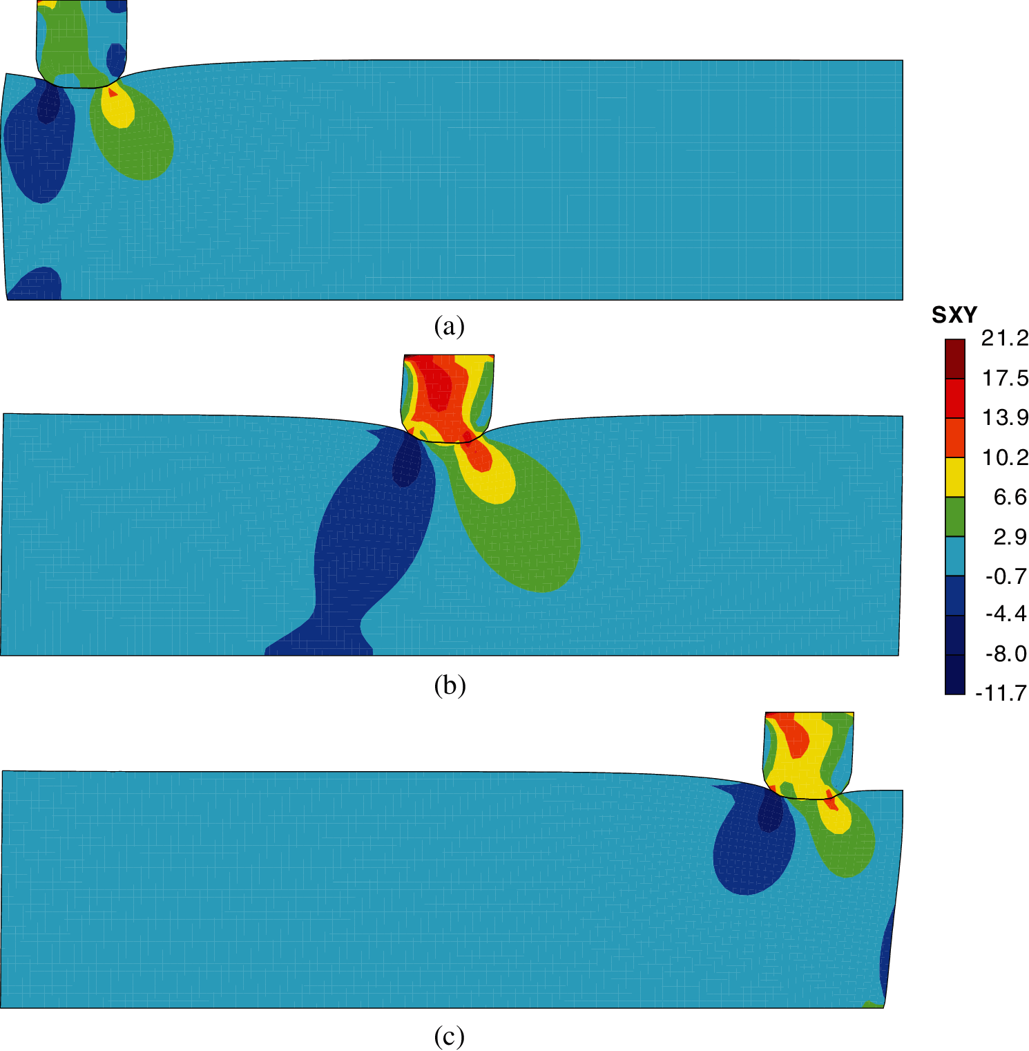
Figure 16: Contour plots of shear stress (unit: MPa) at three instants: (a) 1.0 s; (b) 1.5 s; (c) 2.0 s

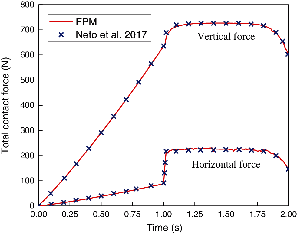
Figure 17: Contact forces obtained by the FPM and surface smoothing method [4]

5.1.2 Contact in Elastoplastic Problem

The second example was proposed by Yang et al. [44] and comprises contact between two curved beams, as shown in Fig. 18. The lower beam is fixed at its bottom surface, while the upper beam is subjected to a horizontal displacement ux= 31.5 mm at its upper surface. Both beams are modeled using an elastoplastic material with isotropic hardening. The elastic material properties are given by Young's modulus E= 689.56 MPa and Poisson's ratio ν = 0.32, while the plastic properties are given by the yield stress σ0= 31 MPa and the plastic modulus h = 261.2 MPa. The density of the material is ρ= 50 kg/m3, and the mass damping coefficient is set to ξ = 1.0 × 104. Each beam is discretized into 240 quadrilateral elements. Both frictionless and frictional cases are investigated, and two different values of the friction coefficient are considered: μ = 0.3 and μ = 0.6. The scale factors for the normal and tangential penalty parameters are set to sn= 10.0 and st = 1.0, respectively.

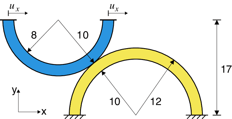
Figure 18: Geometry of the contact problem between two curved beams (unit of length: mm)

Deformed configurations of the beams for 15 mm of prescribed displacement on the upper beam are depicted in Fig. 19 for both frictionless and frictional cases, with the arrows illustrating the nodal contact forces subjected by the lower beam. The contact forces in the frictionless case are normal to the contact surface, while the contact forces in the other two frictional cases comprise tangential components. A higher friction coefficient leads to a higher friction force.

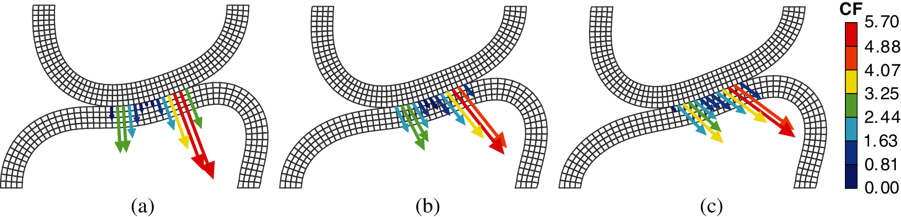
Figure 19: Deformed configurations of the beams and nodal contact forces (unit: N) of the lower beam: (a) μ = 0.0; (b) μ = 0.3; (c) μ = 0.6

The evolution of the total contact force components for the upper beam is presented in Fig. 20. Both the horizontal and vertical contact forces calculated by the FPM agree well with the results obtained by Neto et al. using the surface smoothing method [45]. Given higher values of friction coefficient, the amplitude of contact forces increases, the inflection points of the curves occur later, and contact forces decrease faster. These phenomena are related to the deformation mode of the lower beam due to the friction force.

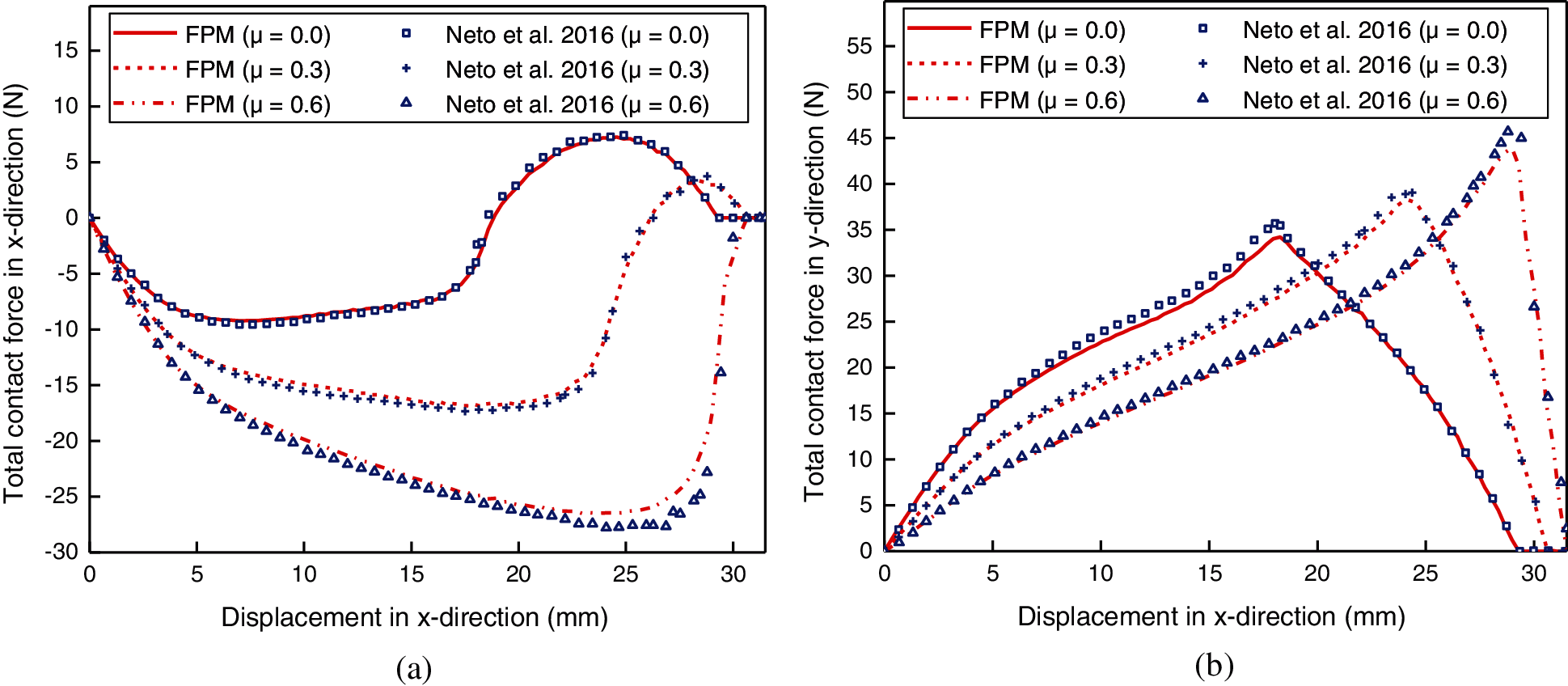
Figure 20: Contact forces obtained by the FPM and surface smoothing method [45]): (a) x-direction; (b) y-direction

The deformed configuration of the beams with contour plots of equivalent plastic strain is presented in Fig. 21, which is similar to the results in the literature [45,46]. The plastic regions mainly appear in the lower beam due to its larger diameter. Besides, the equivalent plastic strain in the region near the contact area is lower given higher values of friction coefficient. This can be explained by the different deformation shapes of the lower beam, as shown in Fig. 19.

Figure 21: Contour plots of equivalent plastic strain: (a) μ = 0.0; (b) μ = 0.3; (c) μ = 0.6

In conclusion, the proposed contact algorithm is also effective in analyzing elastoplastic problems.

5.2 Performance Test

The performance of the proposed method is tested in this section. The performances of parallel element and particle solvers are studied first via a benchmark problem without contact calculation in Section 5.2.1. Then the performance of the parallel contact solver is investigated via a large-scale contact problem in Section 5.2.2. The performances of the parallel FPM solvers are compared with the performances of Abaqus/Explicit solvers and our serial FPM solvers. Note that the kernel codes in the serial FPM solvers are almost identical to the codes in the parallel solvers, but they run serially on a CPU. The efficiency of the parallel implementation is quantified by introducing speedup ratio S, which is defined as

S=TSTP(38)

where TS is the computational time of a serial algorithm, and TP is the computational time of a parallel algorithm.

The quadrilateral element FPM-Q4R in the FPM as described in Section 2.2.4 is used in the performance test, while the 4-node quadrilateral element with reduced integration CPE4R in Abaqus/Explicit is used for comparison. The performance test is carried out on a PC equipped with an Intel® CoreTM i7-4790 K quad-core 4.00 GHz CPU, an NVIDIA Titan V GPU with 5120 CUDA cores and 12 GB HBM2 memory, and a Windows 10 (64-bit platform) operating system.

5.2.1 Test on Parallel Element and Particle Solvers

As shown in Fig. 22, a cantilever beam is fixed at one edge and subjected to a tip load. The load (P = 100 N) is applied at time t = 0 and then kept constant during the whole simulation. The beam is 100 mm long and 20 mm height. It is made of an elastic material characterized by Young's modulus E = 2000 MPa, Poisson's ratio ν = 0.3, and density ρ = 3 × 103 kg/m3. A dynamic analysis of the beam is carried out for 8 ms of simulation. The deformed configuration of the cantilever beam at time t = 8 ms obtained by FPM is presented in Fig. 23. The evolution of the vertical displacement of the cantilever tip obtained by FPM agrees well with that obtained by Abaqus, as shown in Fig. 24.

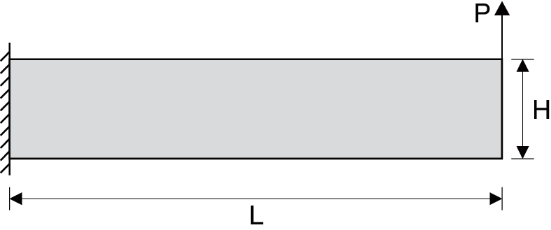
Figure 22: Geometry of cantilever beam

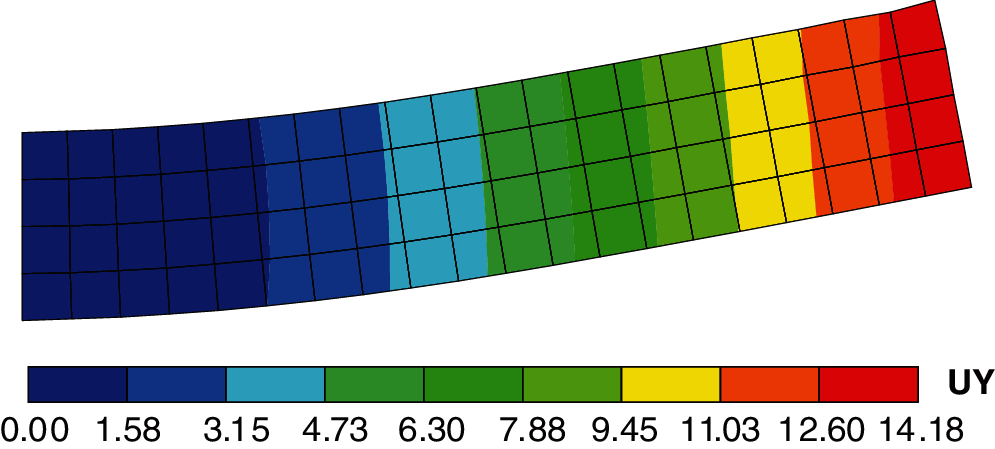
Figure 23: Vertical displacement contour of cantilever beam (unit of length: mm)

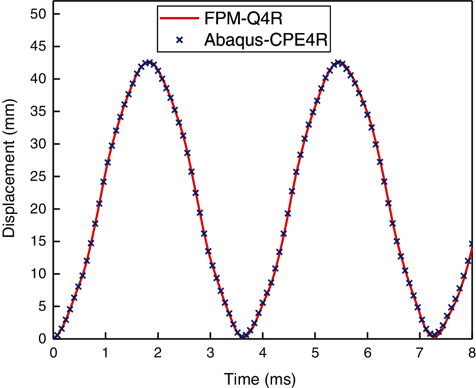
Figure 24: Vertical displacement of the tip node of the cantilever beam

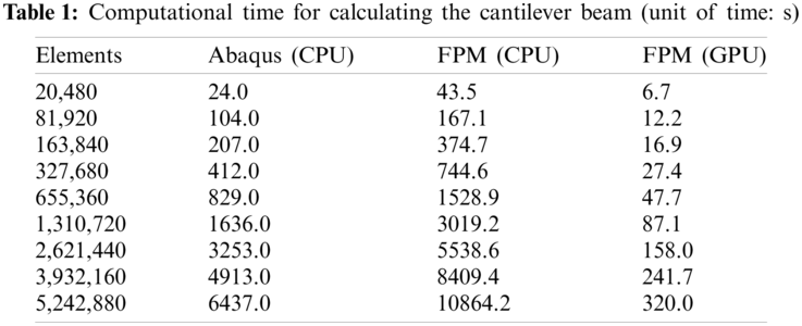
To compare the performances of parallel FPM solvers relative to serial FPM solvers and the Abaqus/Explicit solver, different meshes of the cantilever are tested. Each mesh is performed with a simulation of 0.1 ms with a fixed time step size of 1.0 × 10−5 ms, resulting in 10,000 time increments in total. The computational times taken by Abaqus and FPM are listed in Tab. 1 and compared in Fig. 25. As the number of elements increases, the computational time required by parallel FPM solvers grows at a much lower rate than that of serial FPM solvers and Abaqus solvers. The speedup of parallel FPM solvers relative to serial FPM solvers reaches 35.0 when the number of elements approaches 3,000,000, and the speedup relative to Abaqus reaches 21.7 when the number of elements approaches 4,000,000. The maximum GPU utilization of the parallel element and particle solvers is obtained when the speedup reaches its saturation point, which means that all GPU threads cannot be concurrently processed due to the limitation of GPU memories and cores, and the time consumed by synchronization of threads and other processes leads to the slight decrease of the speedup ratio. If a more advanced GPU with larger memories and more CUDA cores is used, the speedup can be further improved.

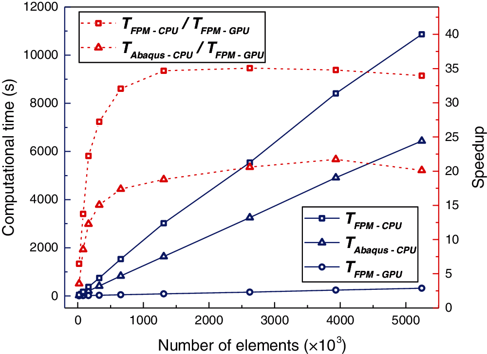
Figure 25: Comparison of computational time for calculating the cantilever beam

5.2.2 Test on Parallel Contact Solver

A two-dimensional simplification of the dynamic impact problem proposed by [38] is considered in this test, as shown in Fig. 26. A half-tube is moving toward a multilayer sheet with a prescribed displacement uy. The sheet is divided into n layers with the same thickness tl, and the gap between two adjacent layers is denoted by gl. The nodes on both the leftmost and rightmost sides of the sheet are fixed only along the vertical direction.

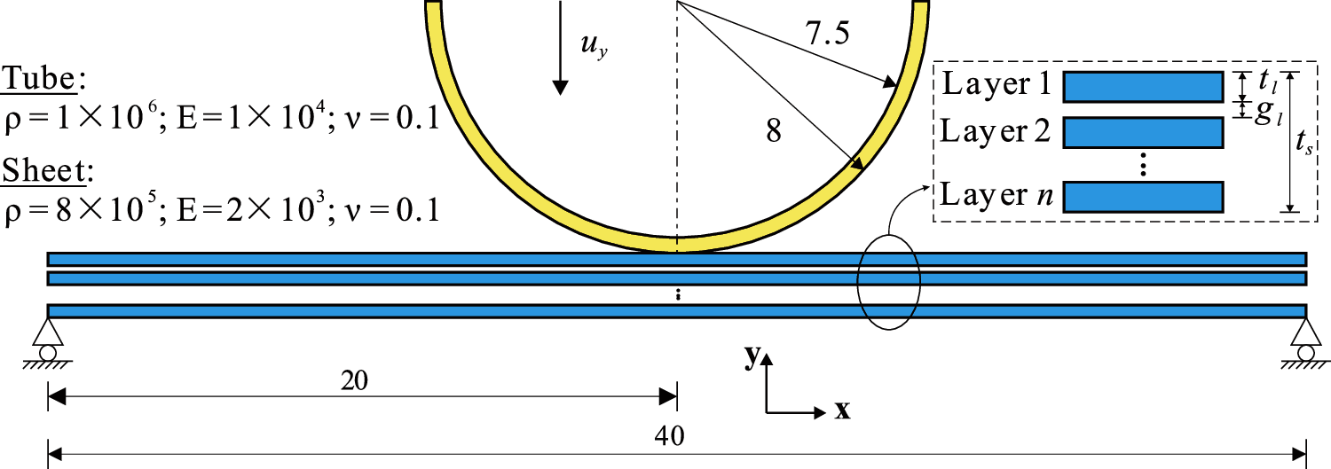
Figure 26: Contact between a half-tube and a multilayer sheet: Geometry and material properties (unit of length: mm; unit of density: kg/m3; unit of modulus: MPa)

A three-layer sheet is taken as an example to demonstrate the results, where tl= 0.4 mm and gl= 0.02 mm. The scale factor for the normal penalty parameter is set to sn= 1.0. The deformed shapes at three instants obtained by FPM are shown in Fig. 27, and they are very similar to the results obtained by Abaqus/Explicit, which are omitted here for brevity.

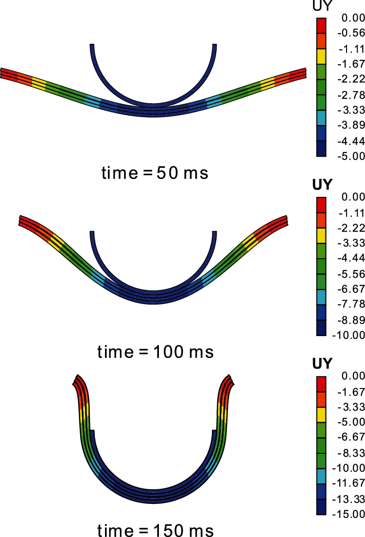
Figure 27: Vertical displacement contour at three instants (unit of length: mm)

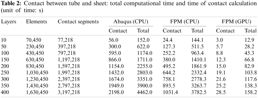
To test the performance and efficiency of the proposed contact algorithm, sheets with different numbers of layers are tested. The layer thickness is set to tl= 0.01 mm and the gap is set to gl= 0.001 mm. The tube is discretized with a fixed mesh size of 0.02 mm, and each layer of the sheet is discretized with a fixed mesh size of 0.01 mm. Each case is performed with a simulation time of 1.0 ms with a fixed time step size of 1.0 × 10−4 ms, resulting in 10,000 time increments in total.

The times of both total calculation and contact calculation taken by Abaqus/Explicit and both serial and parallel FPM solvers are listed in Tab. 2. Note that the time of contact calculation taken by Abaqus/Explicit cannot be extracted directly, and it is approximated by subtracting the time of calculation without contact from the time of calculation with contact.

The computational time of contact calculation and the corresponding speedups are shown in Fig. 28. As the number of contact segments increases, the speedup of the parallel FPM contact solver relative to the serial one increases accordingly and reaches 36.1 when the number of contact segments exceeds 3,000,000, and the speedup relative to the Abaqus contact solver reaches 77.4 when the number of contact segments exceeds 2,000,000. It can be concluded that the serial FPM contact solver is more efficient than the Abaqus contact solver due to the proposed contact algorithm that consists of efficient global search and local search processes. The efficiency of the parallel FPM contact solver is further dramatically improved due to its high degree of parallelism.

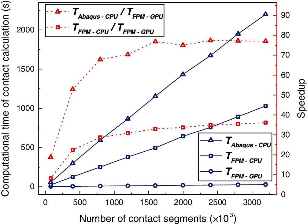
Figure 28: Contact between tube and sheet: computational time of contact calculation

The total computational time and the corresponding speedups are shown in Fig. 29. The speedup of the parallel FPM solvers relative to the serial ones reaches 23.9, and that relative to Abaqus reaches 28.5. Figs. 28 and 29 also indicate that when the number of contact segments exceeds 3,000,000, the GPU cores are fully used. Note that the maximum speedup depends heavily on the GPU hardware, and higher speedup can be achieved by using more advanced GPUs.

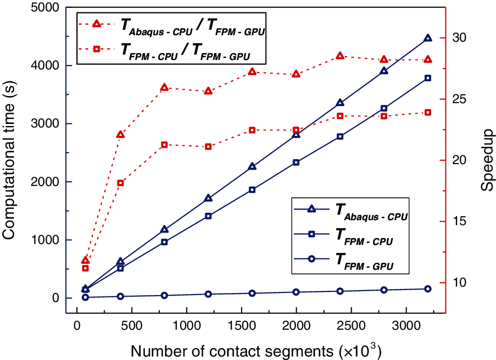
Figure 29: Contact between tube and sheet: total computational time

The percentages of contact calculation time in total calculation time are compared in Fig. 30. As the number of contact segments increases, the three curves remain nearly constant. Contact calculation accounts for approximately 50% of the total computational time in Abaqus, while the percentages in serial and parallel FPMs are only 27% and 18%, respectively. This indicates that the proposed GPU-based parallel contact algorithm can remarkably decrease the time consumption of contact calculation compared to the CPU-based serial contact algorithm.

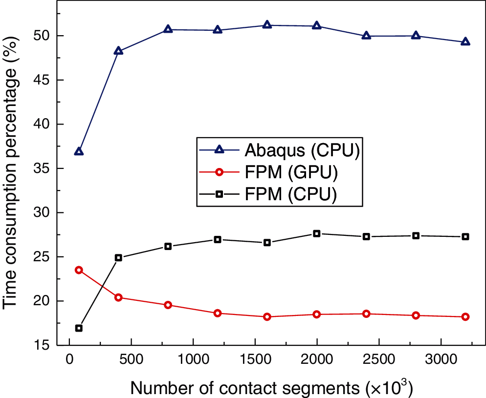
Figure 30: Contact between tube and sheet: time consumption percentages of contact calculation

The time consumption percentages of both serial and parallel FPM solvers are given in Fig. 31. In both serial and parallel cases, the element solvers are the most time-consuming solvers, while the particle solvers account for the smallest proportion. The serial contact solver accounts for a larger proportion than the parallel contact solver, demonstrating the effectiveness of the proposed parallel contact algorithm.

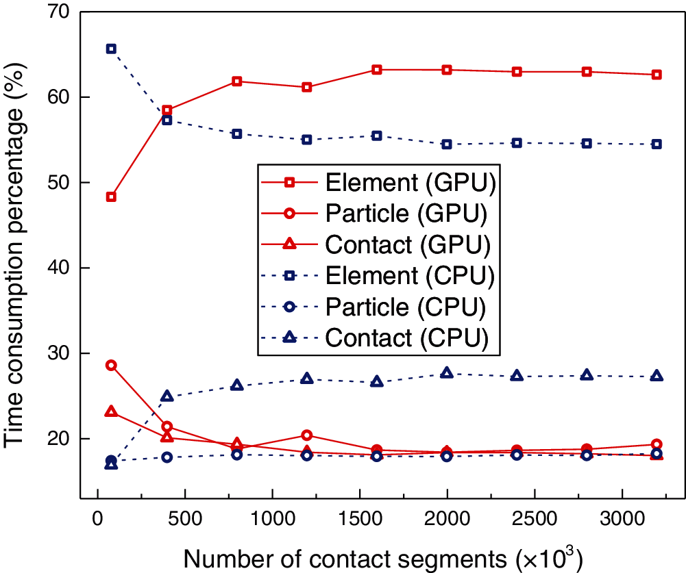
Figure 31: Contact between tube and sheet: time consumption percentages of serial and parallel FPM solvers

6  Conclusions

This paper presents a 2D GPU-based parallel contact algorithm using the FPM. A data structure suitable for parallel contact detection is introduced, and parallel global search and local search procedures are proposed. The main computational procedures, including elemental internal forces calculation, contact calculation, and solution of equations of motion, are executed in parallel on a GPU. Two verification examples and two performance tests are demonstrated, and the following conclusions can be made:

•   Two typical verification examples involving large deformation frictional contacts and both elastic and elastoplastic behaviors are presented, and the results obtained by FPM agree well with those in the literature, indicating the accuracy of the FPM quadrilateral elements and the proposed contact algorithm.

•   The performances of parallel element and particle solvers are studied first via a benchmark problem without contact calculation, and a maximum speedup of approximately 21.7 is achieved relative to Abaqus/Explicit when the number of elements approaches 4,000,000, and a maximum speedup of approximately 35.0 is achieved relative to serial FPM solvers when the number of elements approaches 3,000,000. Thus, the efficiency of the parallel element and particle solvers is proven.

•   A large-scale contact problem is investigated. The speedup of the parallel FPM contact solver relative to the serial FPM contact solver reaches 36.1 when the number of contact segments exceeds 3,000,000, and that relative to the Abaqus contact solver reaches 77.4 when the number of segments exceeds 2,000,000. Thus, the efficiency of the parallel FPM contact solver has been proven. With respect to the total computational time, the speedup of parallel FPM solvers relative to serial FPM solvers reaches 23.9, and that relative to Abaqus reaches 28.5, demonstrating the efficiency of the parallel FPM solvers for solving large-scale contact problems.

•   The percentages of contact calculation time in the total calculation time are 18% in parallel FPM, 27% in serial FPM and 50% in Abaqus/Explicit, which indicates the effectiveness of the proposed GPU-based parallel contact algorithm in reducing the time consumption proportion of contact calculation in the total calculation.

Funding Statement: This work was supported by the National Key Research and Development Program of China [Grant No. 2016YFC0800200]; the National Natural Science Foundation of China [Grant Nos. 51778568, 51908492, and 52008366]; and Zhejiang Provincial Natural Science Foundation of China [Grant Nos. LQ21E080019 and LY21E080022]. This work was also supported by the Key Laboratory of Space Structures of Zhejiang Province (Zhejiang University) and the Center for Balance Architecture of Zhejiang University.

Conflicts of Interest: The authors declare that they have no conflicts of interest to report regarding the present study.

This work is licensed under a Creative Commons Attribution 4.0 International License, which permits unrestricted use, distribution, and reproduction in any medium, provided the original work is properly cited.