Computer Modeling in Engineering & Sciences

DOI: 10.32604/cmes.2021.014960

ARTICLE

Multi-Objective High-Fidelity Optimization Using NSGA-III and MO-RPSOLC

N. Ganesh1, Uvaraja Ragavendran2, Kanak Kalita3,*, Paras Jain4 and Xiao-Zhi Gao5

1Department of Computer Science and Engineering, Vel Tech Multi Tech Dr. Rangarajan Dr. Sakunthala Engineering College, Chennai, 600062, India
2Department of Electronics and Telecommunication Engineering, MPSTME SVKM'S Narsee Monjee Institute of Management Studies, Shirpur, 425405, India
3Department of Mechanical Engineering, Vel Tech Rangarajan Dr. Sagunthala R&D Institute of Science and Technology, Avadi, 600062, India
4School of Computing Science and Engineering, VIT Bhopal University, Sehore, 466114, India
5School of Computing, University of Eastern Finland, Kuopio, 70211, Finland
*Corresponding Author: Kanak Kalita. Email: kanakkalita02@gmail.com
Received: 12 November 2020; Accepted: 03 June 2021

1  Introduction

Composite structures, owing to their superior properties like excellent strength to weight ratios and superb stiffness to weight ratios are steadily replacing steel and other metallic structures in structural engineering. As such, these composite structures often operate in various static and dynamic loading conditions [1]. Often these composite structures carry vibrating machinery/equipment on them. To avoid resonance, it becomes necessary that these structures are designed in such a way that the vibrating equipment operates well outside the first few prominent natural frequencies of the structure.

Simulating the static or dynamic behaviour of laminated composites using numerical methods like finite element analysis (FEA) has achieved a lot of attention. Such high-fidelity numerical methods can be coupled with optimization methods to predict the optimal parameter combinations. For a given design or a specific application, often the geometric parameters of composite plates are unalterable. In such cases, altering the stacking sequence of laminated plates to optimize its performance is the most convenient approach. However, owing to the wide design space, i.e., ply angle range of ±90∘ for each lamina, it is physically impossible to experimentally obtain the optimal combination of ply angles, especially when the number of plies is high. For example, for a symmetric laminated composite plate having 4 layers, i.e., 2 design variables, the total number of possible ply angle combinations is 1812 (considering discrete ply angles with 1∘ increment). Thus, it is clear that the complexity of the search space and its dimension will increase substantially if the number of layers in the composite plate is increased. Adali et al. [2] used a mathematical programming approach to predict the optimal fundamental frequencies in symmetric laminates. Narita [3] used a Ritz-based layerwise optimization approach, which was able to achieve appreciable results with low computational costs. However, as pointed out by Apalak et al. [4], such mathematical methods are often sensitive to gradients and sometimes may get trapped in local optima. Diaconu et al. [5] in a study on thick laminated plates obtained the optimal lamination parameters and corresponding ply angles without encountering any multi-modality.

To address the shortcomings of gradient-based optimizers, many researchers have relied on metaheuristic optimization techniques. Le Riche and Haftka were among the pioneering researchers to use a genetic algorithm (GA) in laminate optimization. They carried out buckling load maximization [6], thickness minimization [7], stacking optimization [8], etc. Apalak et al. [4] carried out stacking sequence optimization to maximize fundamental frequency using an artificial bee colony (ABC) and GA. Hemmatian et al. [9] used an imperialist competitive algorithm (ICA) along with GA and ant colony optimization (ACO) to simultaneously optimize the weight and cost of a rectangular composite plate. They reported that ICA outperformed GA and ACO. Kalita et al. [10] used GA, PSO (particle swarm optimization) and Cuckoo search to simultaneously optimize fundamental frequency and separation between the first two frequencies. However, both Hemmatian et al. [9] and Kalita et al. [10] used a weighted-sum approach to multi-objective optimization. Correia et al. [11] considered stacking sequence as the design variables while maximizing frequency parameters and minimizing strain energy in composite plates with piezoelectric layers. Vo-Duy et al. [12] used non-dominated sorting genetic algorithm II (NSGA-II) in conjunction with a finite element analysis to minimize weight and maximize the frequency of composite plates. Ghasemi et al. [13] used a similar NSGA-II based strategy to minimize the cost of composite shells while increasing their buckling strength. An et al. [14] studied multi-objective optimal designs of hybrid laminates using genetic algorithms. Serhat et al. [15] carried out fundamental frequency, buckling load and effective stiffness maximization using lamination parameters. Serhat et al. [16] also carried out multi-objective optimization of stiffened composite fuselages.

The literature search reveals that though a lot of work on metaheuristic and FEA-based high-fidelity single-objective optimization has been carried out, similar high-fidelity optimization in a multi-objective perspective is rare. A novel particle swarm optimization called RPSOLC (repulsive particle swarm optimization with local search and chaotic perturbation), demonstrated by the author(s) as an effective single optimization tool in their previous works [10,17,18] has been further enhanced to carry out multi-objective Pareto optimization. By comparing with a powerful and recent multi-objective algorithm called the NSGA-III (non-dominated sorting genetic algorithm-III), the efficacy and utility of MO-RPSOSLC in designing laminated composites are demonstrated.

2  Methodology

The methodology used in the current research work is shown in Fig. 1. Laminated composite plate design considering multiple natural frequency criteria is considered as the design problem. The design problem is introduced in detail in Section 2.1. The ply orientations of the individual lamina are selected as the design variables. A finite element module is developed in Fortran language that can accurately determine the natural frequencies of the laminated plate. The finite element formulation is discussed in detail in Section 2.2. Next, two independent multi-objective optimization modules (NSGA-III and MO-RPSOLC) for carrying out Pareto optimization are developed in Fortran. These are discussed in detail in Sections 2.3 and 2.4, respectively. The FEM module is incorporated as the objective function in the NSGA-III and MO-RPPSOLC modules. Over several generations, the Pareto solutions are iteratively improved by the optimization techniques. The Pareto fronts by the NSGA-III and MO-RPSOLC are compared and the superior one is selected. Further, suitable compromise solutions relating to various test cases are selected by using a multi-criteria decision-making method called TOPSIS. The details of the TOPSIS are discussed in Section 2.5.

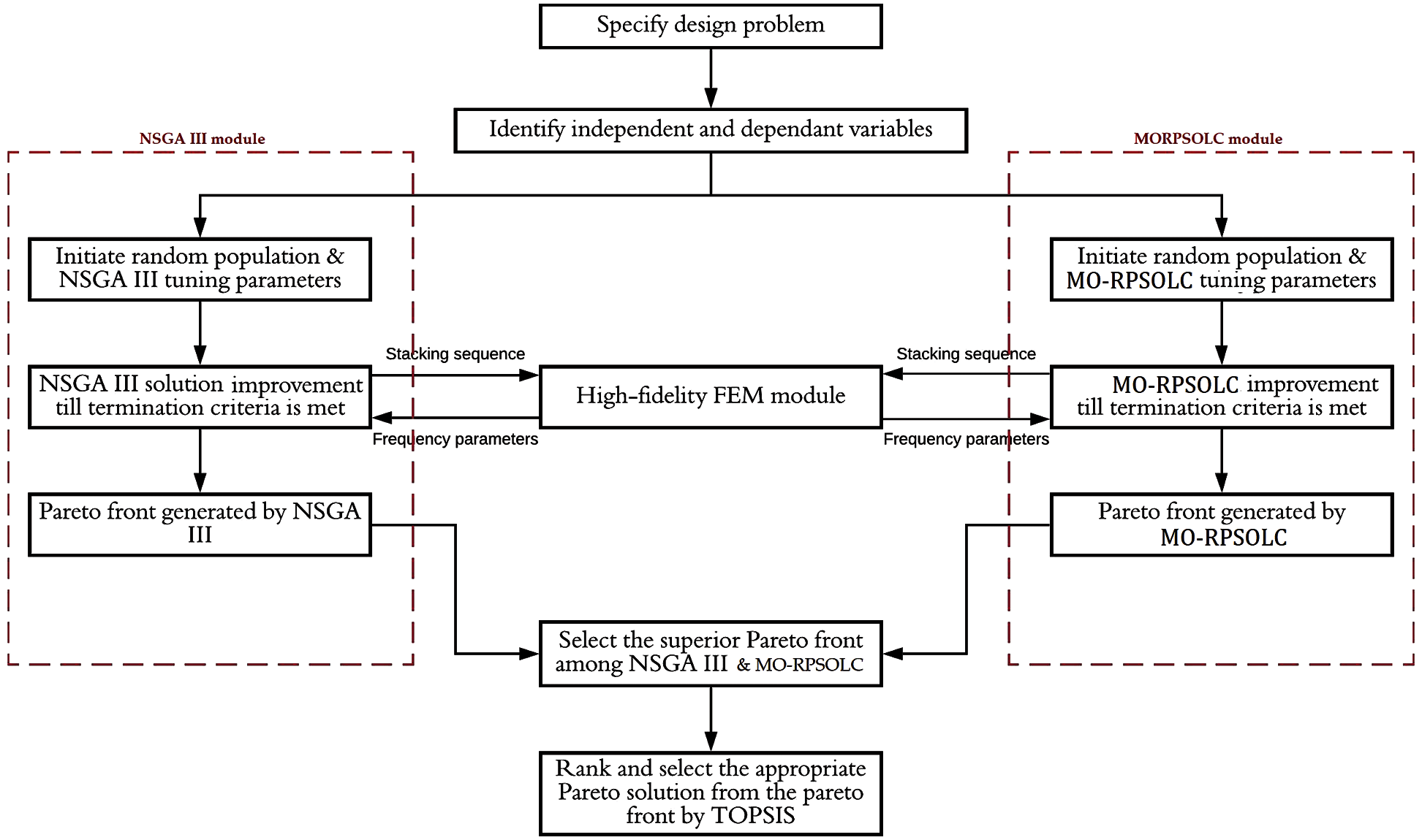
Figure 1: The methodology used in the current research work

2.1 Problem Statement

In this paper, laminated composite plates of the configuration as shown in Fig. 2 is used. An eight-ply square (ba=1) symmetric Graphite-epoxy [19] composite laminate having a thickness (h=0.01) and material properties as follows is considered:

E1=138 GPa,E2=8.96 GPa,G12=7.1 GPa,υ12=0.3.

The boundary condition at the edges of the plates may be clamped (C), simply supported (S) or free (F). Based on these conditions, 18 different boundary condition combinations are considered for the laminated plates.

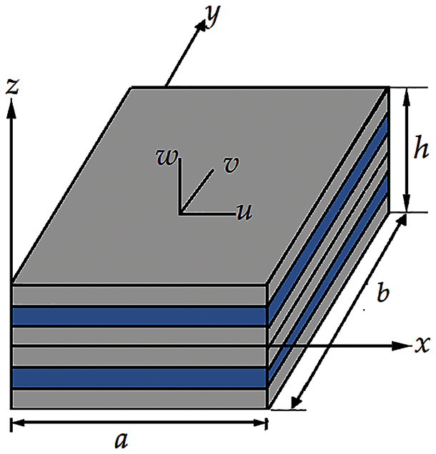
Figure 2: Typical laminated plate considered in the study

The fundamental frequency (λ1) and the difference between the first two natural modes (λ21) are to be maximized simultaneously. The stacking sequence (i.e., the ply angles denoted by θ) of the laminated composites are considered as the design variables to achieve this multi-objective optimization. Optimizing the stacking sequence of laminated composite plates to optimize its performance is a combinatorial optimization problem, which may be stated as,

Find θi=(θ1,θ2,θ3 and θ4)

which maximizes λ1=f(θi) and λ21=f(θi) (1)

subject to−90∘≤θi≤90

As such two powerful metaheuristic optimization algorithms—NSGA-III and MO-RPSOLC are used. Both these algorithms independently generate a set of non-dominated solution known as the Pareto front. Each solution within the Pareto front is a compromise multi-objective solution. Since the frequency parameters are quite sensitive to the stacking sequence, a high-fidelity finite element analysis is carried out which runs in conjunction with the optimization algorithms.

2.2 Finite Element Method Formulation

In this work, high-fidelity structural analysis of the laminated composite plates is carried out using a highly accurate finite element analysis (FEA) module. In past, this FEA module has been used by Kalita et al. [1] to accurately compute the Eigen frequencies in taper plates, laminated plates [20] and isotropic plate with holes [21].

The FEA module is based on a nine-node isoparametric plate bending element. The element contains four corner nodes, four mid-edge nodes and one centre node. The effect of shear deformation is an important consideration for laminated composites since they are weak in shear. This is included in the current FEA module by assuming the considerations of FSDT (First-order Shear Deformation Theory) which states that the normal to the midplane would remain straight after deformation but may or may not remain normal.

{ϕxϕy}={θx−∂w∂xθy−∂w∂y} (2)

where ϕx and ϕy represent the average shear rotation over the entire plate thickness and θx, while θy are denote total rotations in bending. u, v are the in-plane displacements whereas w is the transverse displacement.

u=∑r=19Nrur

v=∑r=19Nrvr

w=∑r=19Nrwr (3)

θx=∑r=19Nrθxr

θy=∑r=19Nrθyr

The nine-node isoparametric plate bending element maps the laminated plate by using the following equations:

x=∑r=19Nrxr

y=∑r=19Nryr (4)

where (x,y) is the location of any given point within the element, the rth nodal point’s location within the element is given by (xr,yr) and the assumed Lagrangian interpolation function is denoted as Nr.

For any composite laminate, the stress-strain relation can be expressed as,

{σ}=[D]{ε} (5)

{σ} is the generalized stress vector.

{σ}T=[NxNyNxyMxMyMxyQxQy] (6)

where the in-plane force resultants are represented as Nx,Ny,Nxy; bending moments in the x and y directions are indicated as Mx,My; the twisting moment resultant is indicated as Mxy. Qx,Qy are the transverse shear force resultants.

In terms of displacement fields, the strain vector is,

{ε}T=[∂u∂xdvdy∂u∂y+∂v∂x−∂θx∂x−∂θy∂y−∂θx∂y−∂θy∂x∂w∂x−θx∂w∂y−θy] (7)

[D]=[A11A12A16B11B12B1600A12A22A26B12B22B2600A16A26A66B16B26B6600B11B12B16D11D12D1600B12B22B26D12D22D2600B16B26B66D16D26D6600000000kc.A55kc.A54000000kc.A45kc.A44] (8)

where, Aij=∑k=1n(Qij)k(Zk+1−Zk) (9)

Bij=12∑k=1n(Qij)k(Zk+12−Zk2) (10)

Dij=13∑k=1n(Qij)k(Zk+13−Zk3) (11)

Aij,Bij and Dij represent the extensional stiffness, extensional-bending stiffness and bending stiffness coefficients respectively. The number of individual laminas forming the composite plate is indicated as n. The material coefficients of the kth layer are denoted as (Qij)k.

Q11k=E11−μ12μ21;Q22k=E21−μ12μ21;Q12k=Q21k=μ12E21−μ12μ21

Q44k=G23;Q55k=G13;Q66k=G12 (12)

μ21E1=μ12E2 (13)

where E1 and E2 are the longitudinal and transverse Young’s modulus, respectively. μ12 and G12,G13,G23 are the in-plane Poisson’s ratio and shear moduli, respectively.

The strain vector can be summarized as,

{ε}=∑r=19[∂Nr∂x00000∂Nr∂y000∂Nr∂y∂Nr∂x000000−∂Nr∂x00000−∂Nr∂y000−∂Nr∂y−∂Nr∂x00∂Nr∂x−Nr000∂Nr∂y0−Nr]{urvrwrθxrθyr} (14)

i.e., {ε}=∑r=19[B]r{δr}e (15)

or {ε}=[B]{δ} (16)

[K]e=∫−1+1∫−1+1[B]T[D][B]|J|dξdη (17)

where [B] is the strain matrix, {δ} is the nodal displacement vector and [K] is the stiffness matrix. |J| is the Jacobian matrix.

The lumped mass matrix is computed as,

[M]=ρh∫−1+1∫−1+1[[Nu]T[Nu]+[Nv]T[Nv]+[Nw]T[Nw]+h212[Nθx]T[Nθx]+h212[Nθy]T[Nθy]]×|J|dξdη (18)

where,

[Nu]=[[Nr][N0][N0][N0][N0]]

[Nv]=[[N0][Nr][N0][N0][N0]]

[Nw]=[[N0][N0][Nr][N0][N0]]

[Nθx]=[[N0][N0][N0][Nr][N0]]

[Nθy]=[[N0][N0][N0][N0][Nr]]

where [N0] is a null matrix of the order 1×9.

[Nu]T[Nu] and [Nv]T[Nv] are responsible for the in-plane movements of mass. [Nw]T[Nw] is related to inertia is the transverse movement of mass. h212[Nθx]T[Nθx] and h212[Nθy]T[Nθy] are responsible for rotary inertia.

[K0] and [M0] are the overall stiffness matrix and mass matrix respectively. The plates’ equation of motion is,

[K0]=ω2[M0] (19)

where ω is the frequency of the plate, calculated by solving Eq. (19) using the simultaneous iterative technique. In this article, all the frequency parameters are expressed in non-dimensional form as,

λ=ωa2ρh/D0,where,D0=E2h312(1−υ12υ21) (20)

Kalita et al. [1,21] in their previous works has shown that the current FEM formulation can determine the natural frequencies with less than 1% error as compared to higher-order shear deformation theory and analytical solutions for thin and moderately thick plates. A mesh size of 18 × 18 was found to be satisfactory in those studies. However, in the current work, to keep the computational time manageable, a reduced mesh of 4 × 4 is used as shown in a previous optimization study [18] by the author(s).

2.3 Optimization with NSGA-III

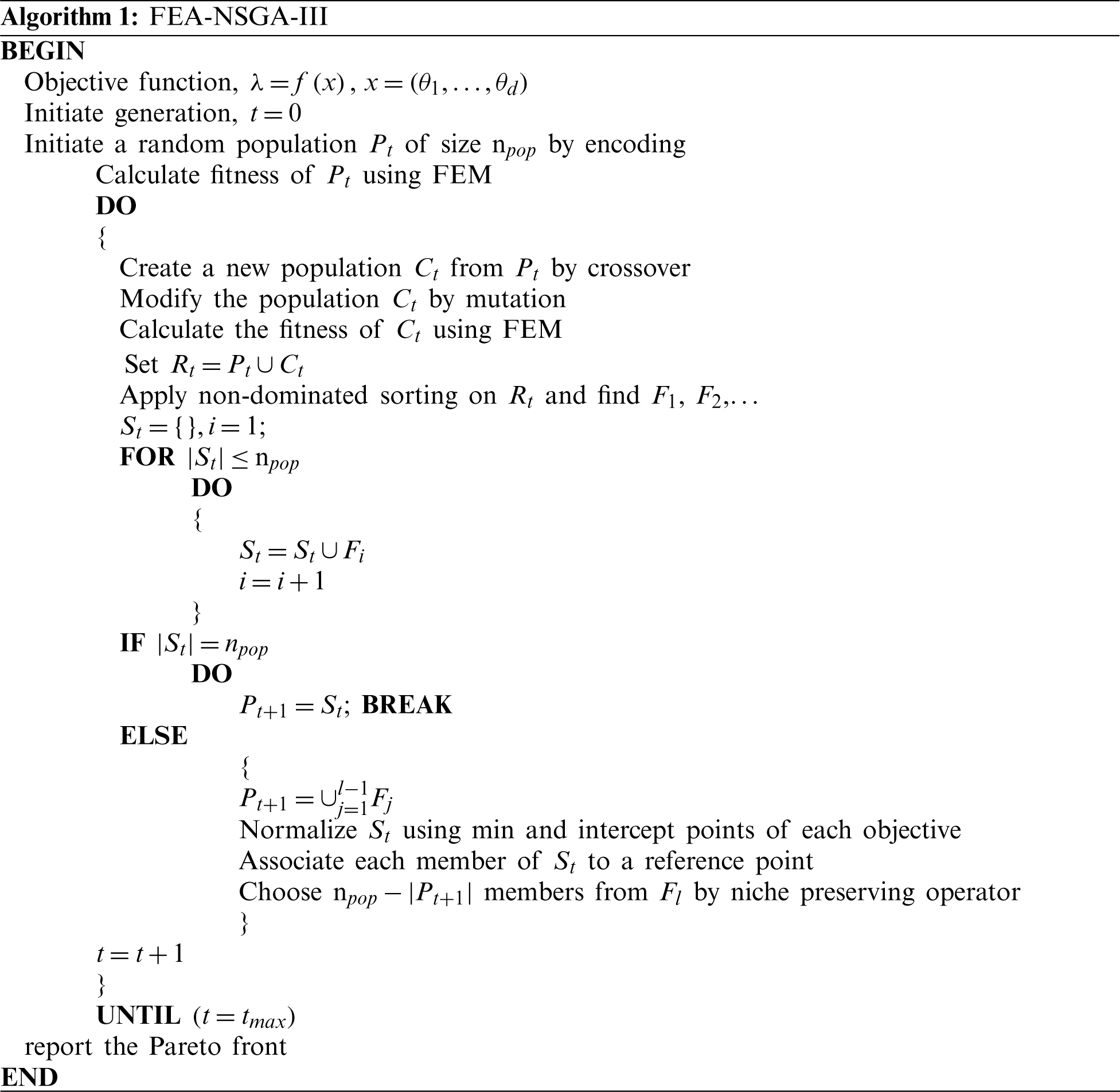
In this work, the non-dominated sorting genetic algorithm III (NSGA-III) [22,23] is used for carrying out Pareto optimization. The multi-objective optimization problem is stated in Eq. (1). The NSGA-III is based on Darwin’s theory of natural evolution. The algorithm starts by assuming a set (called population) of possible solutions (called individuals). Each individual has certain properties (called chromosomes) which can be combined with others, mutated and thus, improved. These improvements in the fitness of the individuals go on until a termination criterion is met. The FEA-NSGA-III used in the current research is realized by using the pseudo-code given in Algorithm 1.

2.4 Optimization with MO-RPSOLC

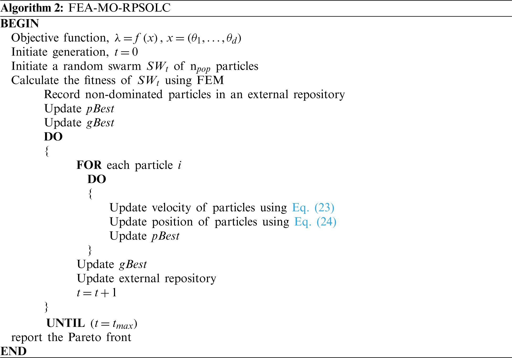
In this article, a novel memetic version of PSO (Particle Swarm Optimization) called RPSOLC (Repulsive Particle Swarm Optimization with Local Search and Chaotic Perturbation) is used for multi-objective optimization of laminated composites. In past, single-objective RPSOLC has been used by Kalita et al. [17] for optimizing the laminated composites. Kalita et al. [10] has also used RPSOLC to conduct weighted sum multi-objective optimization. However, this the first instance of its usage in the Pareto optimization scenario. The architecture used for selecting the Pareto optimal solutions in the current MO-RPSOLC (multi-objective RPSOLC) is similar to that used by Coello et al. [24]. The working of the RPSOLC algorithm is explained below:

Any typical PSO algorithm [25] starts by generating a set of random solutions (called particles) in the design space. In PSO terminology, this set of solutions is collectively called the swarm. Each particle within the swarm is aware of its personal best position called the pBest. The particles in the swarm are also aware of the overall best position (or solution) found so far called the gBest. All particles try to move towards the gBest position by using the following two rules to update their velocity and position.

vt+1=ω.vt+c1.r1.(pBest−xt)+c2.r2.(gBest−xt) (21)

xt+1=xt+vt+1 (22)

where vt and vt+1 are the velocity in the current and the next generation, respectively. Similarly, xt and xt+1 are the positions of the particle in the current and the next generation, respectively. r1 and r2 are two random number between 0 to 1. c1 and c2 are called the cognitive and social parameters. The effect of the velocity of the previous generation on the velocity of the current generation is controlled by the inertia weight ω.

Due to the traditional PSO’s tendency to get stuck in local optima, Urfalioglu [26] proposed the RPSO in which the particles update their velocity using the relation below:

vt+1=ω.vt+α.r1.(pBest−xt)+ω.β.r2.(pBest¯−xt)+ω.γ.r3.vtr (23)

where α,β,γ are constants. The term α.r1.(pBest−xt) leads any particle towards its self-best position. The term ω.β.r2.(pBest¯−xt) leads the particle away from a randomly chosen particle from the swarm. The term ω.γ.r3.vtr is responsible for the exploration of new search regions.

The traditional RPSO was further upgraded by incorporating the memetic attributes suggested by Santos et al. [27,28]. Each particle is endowed with the ability to conduct a local search by visiting its surroundings. The visit is independent of the gradient in any directions and thus, free from bias. If any particle is seen to be trapped in one position even after a pre-defined number of generations, a small random disturbance in its velocity (called the chaotic perturbation) is inserted.

xt+1=xt+vt+1.(1+rchaos) (24)

where rchaos is the chaotic perturbation. This helps the RPSOLC algorithm to avoid getting trapped in local optima pits. The pseudocode of the current FEA-MO-RPSOLC approach is shown in Algorithm 2.

2.5 Multi-Criteria Decision Making with TOPSIS

For an MCDM problem consisting of m alternatives and n criteria, let D=xij be a decision matrix, where xij∈R. The Pareto fronts obtained from NSGA-III and MO-RPSOLC are used as the decision matrix in this paper.

D=[x11x12⋯x1nx21x22⋯x2n⋮⋮⋱⋮xm1xm2⋯xmn] (25)

There are different objective and subjective weight allocation methods. In this paper, the standard deviation approach described in the preceding section is used. The weight vector may be expressed as,

wj=[w1…wn],where,∑j=1n(w1…wn)=1. (26)

A normalized decision matrix nij of each criterion is created using Eq. (27),

nij=xij∑i=1mxij2 (27)

Next, the weighted normalized matrix is created using Eq. (28),

Nij=wj∗nij for i∈[1,m] and j∈[1,n] (28)

The ideal positive (best) and ideal negative (worst) solutions are then estimated using Eqs. (29) and (30), respectively.

Aj+={max.Nij∣j∈Bmin.Nij∣j∈C (29)

Aj+={min.Nij∣j∈Bmax.Nij∣j∈C (30)

where B is a vector of benefit function and C is the vector of the cost function, for i∈⌈1,m⌉ and j∈⌈1,n⌉.

The separation measurement and relative closeness coefficient are then determined. In TOPSIS, the difference of each response from the ideal positive (best) solution is given by Eq. (31).

Si+=∑j=1n(Nij−Aj+)2 (31)

for i∈[1,m] and j∈[1,n]

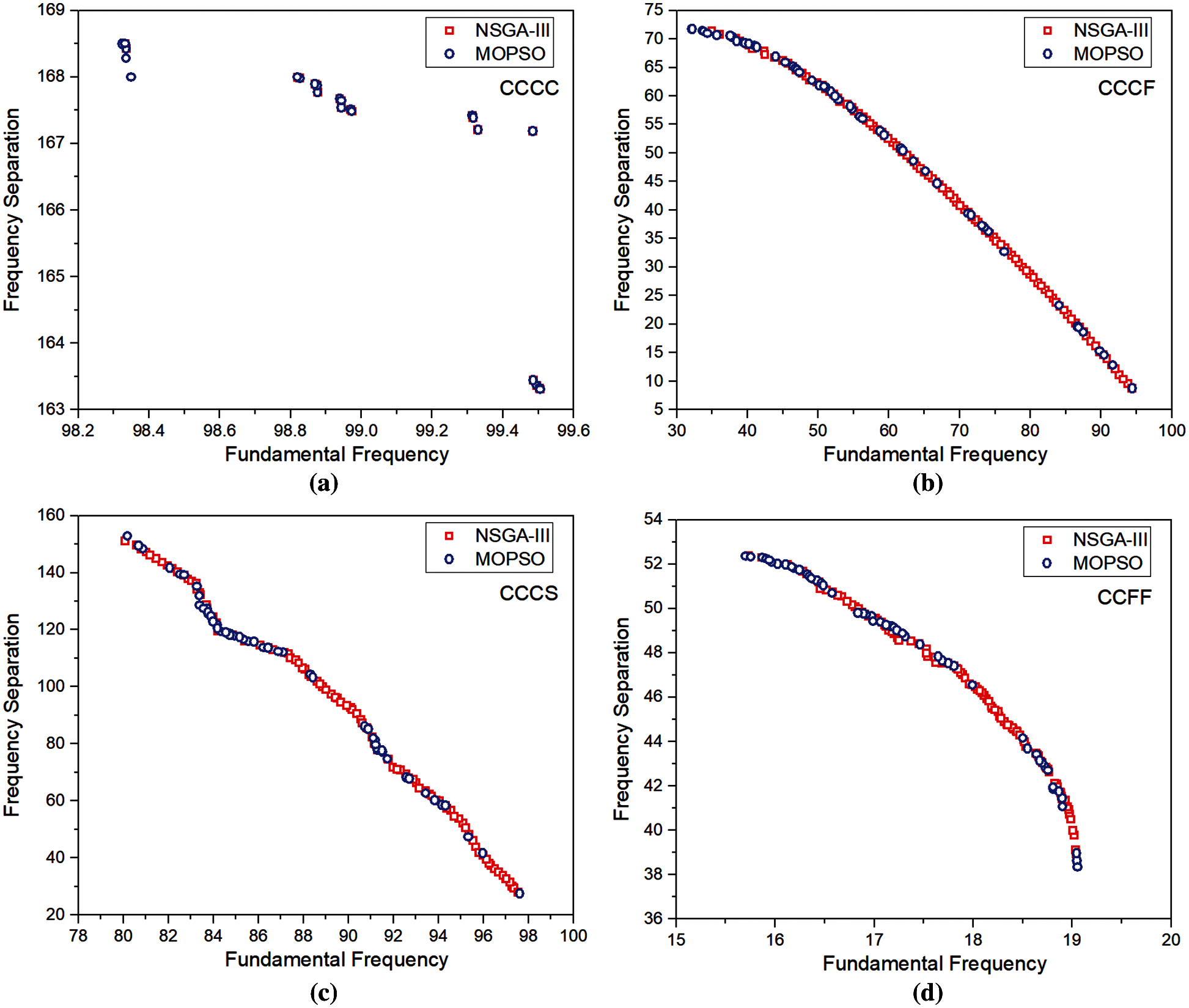
Figure 3: Pareto front by NSGA III and MO-RPSOLC for (a) CCCC (b) CCCF (c) CCCS (d) CCFF

Similarly, the difference between each response from the ideal negative (worst) solution is given by Eq. (32).

Si−=∑j=1n(Nij−Aj−)2 (32)

for i∈[1,m] and j∈[1,n]

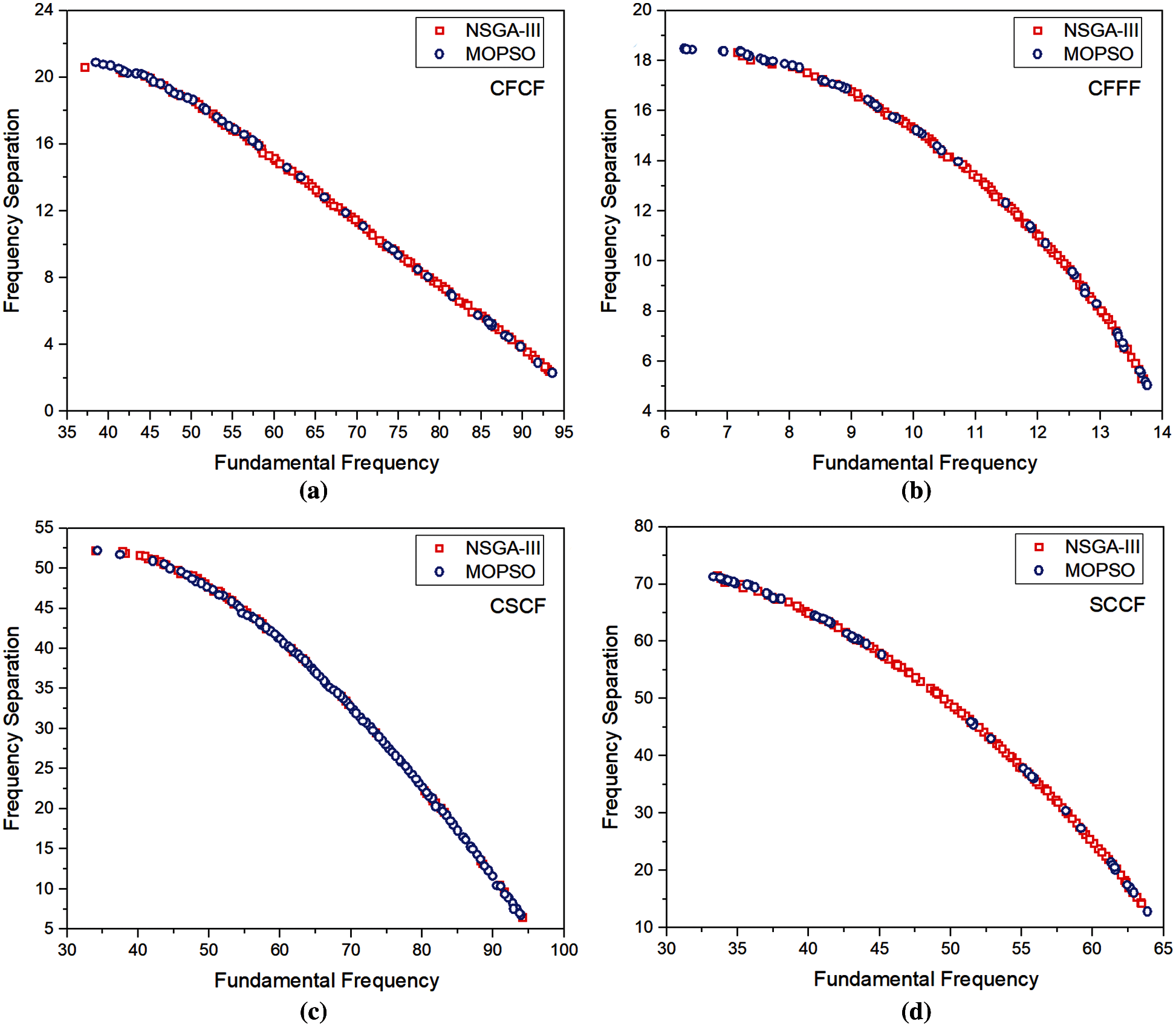
Figure 4: Pareto front by NSGA III and MO-RPSOLC for (a) CFCF (b) CFFF (c) CSCF (d) SCCF

The corresponding closeness coefficient (CCi) of the ith alternative is calculated using Eq. (33).

CCi=Si−Si++Si− (33)

where 0≤CCi≤1, i∈[1,m]

The final step is to rank the alternatives in decreasing order of closeness coefficient value.

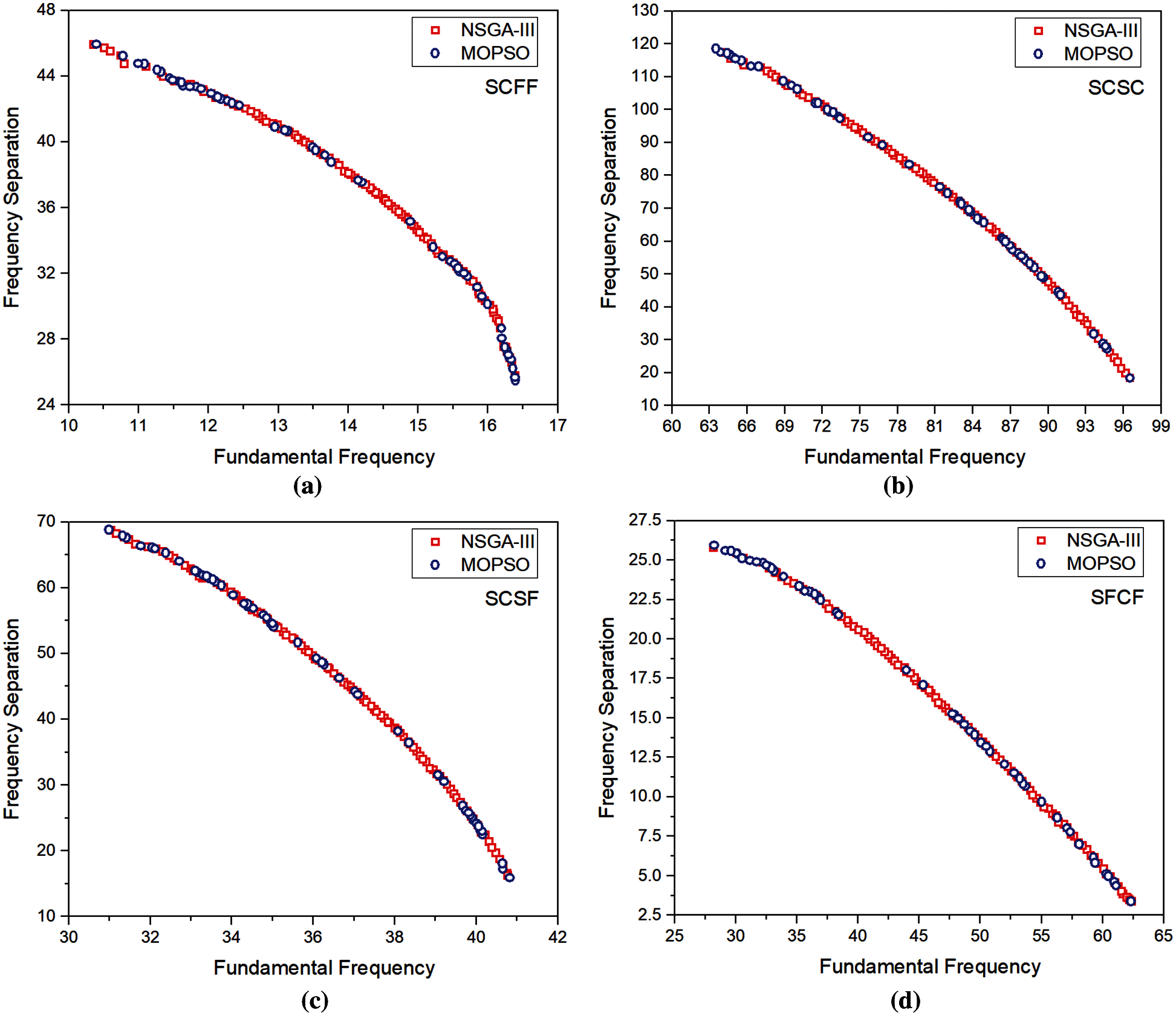
Figure 5: Pareto front by NSGA III and MO-RPSOLC for (a) SCFF (b) SCSC (c) SCSF (d) SFCF

3  Results and Discussion

Figs. 3–7 show the high-fidelity Pareto fronts generated by the NSGA-III and MO-RPSOLC algorithms for 18 different boundary conditions. It is seen that despite the geometric configuration and the material of the laminated composites being the same, in these 18 cases, the boundary condition plays a significant role in the shape of the Pareto fronts. For instance, in cases like CCCC, CCSS, SSSS, etc. the Pareto fronts are discontinuous whereas, in the case of boundary condition combinations like CCCF, CSCF, SCSC the Pareto fronts are smooth and continuous. The discontinuity in Pareto fronts has perhaps arisen due to the algorithm encountering the concave portion of the objectives. This has led to the presence of regions of the objective functions where they are dominated. The severe discontinuity in Pareto fronts in CCCC SSCC, SSFF and SSSS boundary conditions indicates that the presence of several distinct feasible regions with gaps where the solutions are dominated.

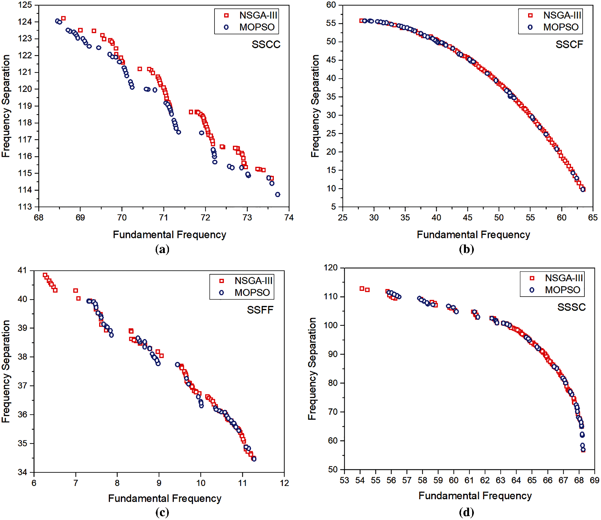
Figure 6: Pareto front by NSGA III and MO-RPSOLC for (a) SSCC (b) SSCF (c) SSFF (d) SSSC

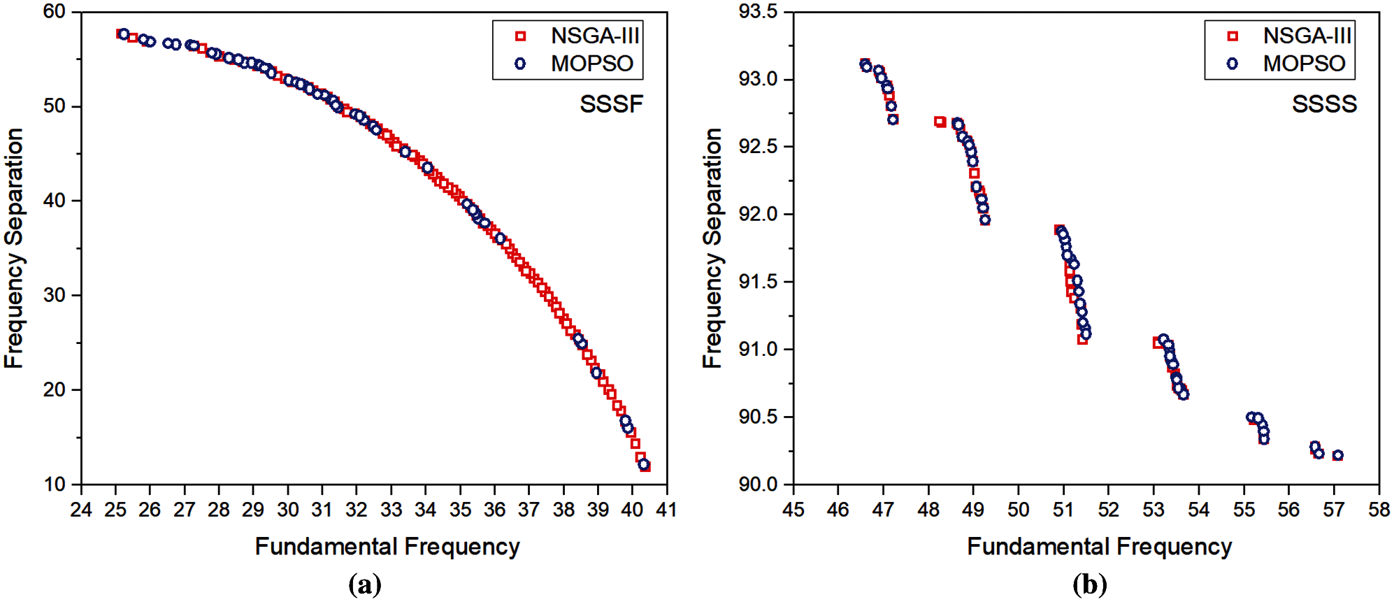
Figure 7: Pareto front by NSGA III and MO-RPSOLC for (a) SSSF (b) SSSS

The optimal stacking sequences corresponding to the limits of the Pareto fronts for different boundary condition cases are reported in Tab. 1. It is seen that in general, the limits of the Pareto fronts for both NSGA-III and MO-RPSOLC show negligible variation. However, it is interesting to observe that the optimal ply angles reported by NSGA-III and MO-RPSOLC mostly vary by either (approx.) 5° or in the orientation direction (±) of the fibre.

The performance of the NSGA-III and MO-RPSOLC in terms of the spread of the Pareto fronts for all the 18 combinations of boundary conditions is shown in Fig. 8. It is seen that in general, the NSGA-III has better uniformity in the Pareto solution spread as compared to the MO-RPSOLC. In most cases, the MO-RPSOLC solutions spread is seen to be skewed. This in contrast to the NSGA-III’s uniformity in the spread, indicates that perhaps the MO-RPSOLC has not explored the design space sufficiently. However, in all the cases the extremum points of the Pareto fronts for both the NSGA-III and MO-RPSOLC seems to be similar. It is also evident from Figs. 8a, 8c and 8e that as the constraints increase the average (of the Pareto front range) fundamental frequency increases. This is because the increase in constraints (i.e., restrictions on the degree of freedoms) causes an increase in the stiffness of the structure which, in turn, is responsible for the increased fundamental frequency. As seen from Figs. 8b, 8d and 8f, baring a few exceptions like CCCC, SSCC boundary condition combinations, as the constraints increase, the range of the frequency separation between the first two natural frequencies also increase. It is worth pointing out here that the average time taken for MO-RPSOLC simulations is approximately 2/3rd of the time taken by NSGA-III. On average, it took 265 min to carry out each NSGA-III simulation on a Dell Inspiron 15-3567 series windows system with Intel(R) CoreTM i7-7500U CPU @ 2.70 GHz, Clock Speed 2.9 Ghz, L2 Cache Size 512 and 8 GB ram.

TOPSIS is used to select the best solutions from the Pareto fronts based on three different test cases. In test case 1, only the ranked 1 solution by TOPSIS is considered; in test case 2, the top 3 ranked solutions are considered. Similarly, for test case 3, the top 10 ranked TOPSIS solutions from the combined Pareto fronts are considered. Additionally, to draw unbiased and comprehensive conclusions based on the TOPSIS analyses, the criteria weight w1 is varied from 0.01 to 0.99 with 0.01 increments for all the boundary conditions. Based on the considered test cases, the optimum predictions for each w1 is recorded.

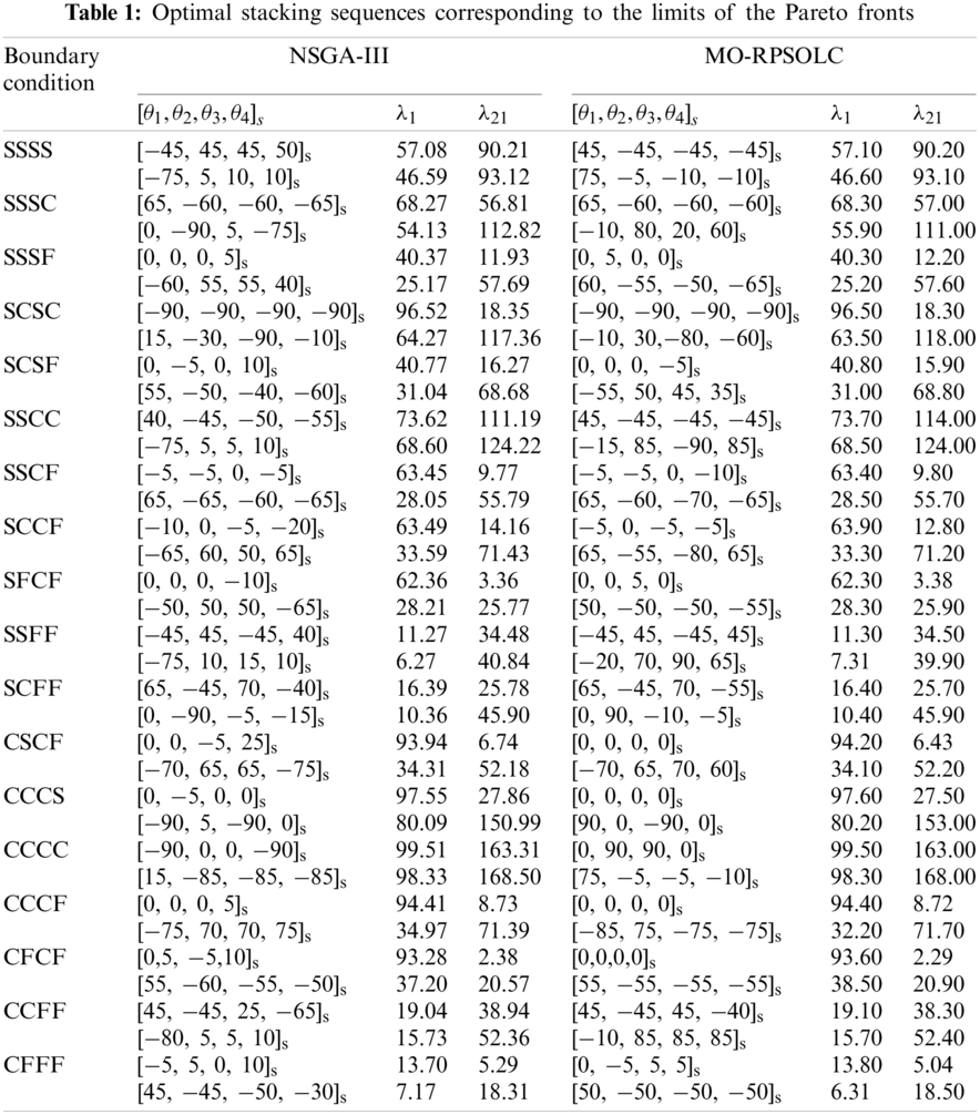
Figure 8: Spread of the Pareto fronts for all 18 boundary conditions

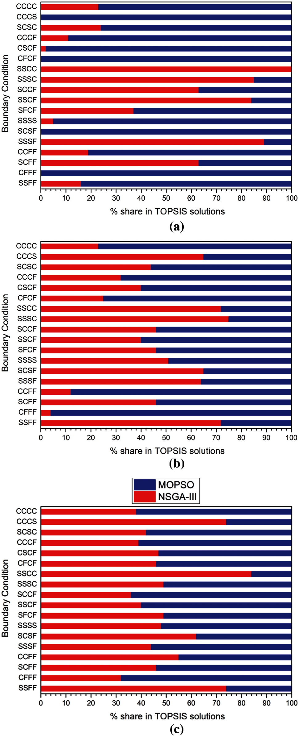
Figure 9: The percentage share of NSGA-III and MO-RPSOLC in TOPSIS selected best solutions considering (a) test case 1: ranked 1 solution (b) test case 2: ranked 1–3 solutions (c) test case 3: ranked 1–10 solutions

The percentage share of the NSGA-III and MO-RPSOLC solutions in the TOPSIS selected optimal solutions (99 in total, 1 solution for each w1 considering test case 1 is calculated and shown in Fig. 9a. It is seen that, in general, MO-RPSOLC solutions have a higher share in the TOPSIS selected optimal solutions. However, in the instances of SSCC, SSSC, SSCF, SSSF, SCCF and SCFF boundary conditions NSGA-III solutions find better representation. Similarly, in Fig. 9b, the TOPSIS selected the top 3 optimal solutions for each w1 is recorded. The share of NSGA-III solutions in the TOPSIS selected optimal solutions is seen to have significantly improved as compared to test case 1. Similar improvement for NSGA-III is seen in Fig. 9c for test case 3 considering TOPSIS selected top 10 optimal solutions.

4  Conclusion

In this research, two popular nature-inspired multi-objective optimization algorithms are evaluated based on their performance in a high-fidelity application. A combinatorial optimization problem of maximizing the first frequency and the difference between the first two natural frequency by optimizing the stacking sequence is chosen. The optimization problem is carried out for 18 different boundary condition combinations. The performance of the algorithms is compared based on the spread of their Pareto solutions as well as by using a novel TOPSIS-based analysis. The comprehensive analysis carried out on the 18 different test cases indicates the MO-RPSOLC to be on par with the reliable and widely used NSGA-III. It is worth mentioning that this is the first instance of using a high-fidelity finite element analysis in conjunction with NSGA-III or MO-RPSOLC to design an optimized structure. Based on the encouraging results of the article it can be concluded that this methodology can be effectively used to predict highly accurate and optimized structural designs which would lead to significant savings in terms of prototype testing.

Acknowledgement: Authors acknowledge the support of their respective institutes.

Funding Statement: The authors received no specific funding for this study.

Conflicts of Interest: The authors declare that they have no conflicts of interest to report regarding the present study.

References

 1.  Kalita, K., Haldar, S. (2017). Eigenfrequencies of simply supported taper plates with cut-outs. Structural Engineering and Mechanics: An International Journal, 63(1), 103–113. DOI 10.12989/sem.2017.63.1.103. [Google Scholar] [CrossRef]

 2.  Adali, S., Verijenko, V. E. (2001). Optimum stacking sequence design of symmetric hybrid laminates undergoing free vibrations. Composite Structures, 54(2–3), 131–138. DOI 10.1016/S0263-8223(01)00080-0. [Google Scholar] [CrossRef]

 3.  Narita, Y. (2003). Layerwise optimization for the maximum fundamental frequency of laminated composite plates. Journal of Sound and Vibration, 263(5), 1005–1016. DOI 10.1016/S0022-460X(03)00270-0. [Google Scholar] [CrossRef]

 4.  Apalak, M. K., Karaboga, D., Akay, B. (2014). The artificial bee colony algorithm in layer optimization for the maximum fundamental frequency of symmetrical laminated composite plates. Engineering Optimization, 46(3), 420–437. DOI 10.1080/0305215X.2013.776551. [Google Scholar] [CrossRef]

 5.  Diaconu, C. G., Sato, M., Sekine, H. (2002). Layup optimization of symmetrically laminated thick plates for fundamental frequencies using lamination parameters. Structural and Multidisciplinary Optimization, 24(4), 302–311. DOI 10.1007/s00158-002-0241-z. [Google Scholar] [CrossRef]

 6.  Riche, R. L., Haftka, R. T. (1993). Optimization of laminate stacking sequence for buckling load maximization by genetic algorithm. AIAA Journal, 31(5), 951–956. DOI 10.2514/3.11710. [Google Scholar] [CrossRef]

 7.  Le Riche, R., Haftka, R. T. (1995). Improved genetic algorithm for minimum thickness composite laminate design. Composites Engineering, 5(2), 143–161. DOI 10.1016/0961-9526(95)90710-S. [Google Scholar] [CrossRef]

 8.  Grosset, L., LeRiche, R., Haftka, R. T. (2006). A double-distribution statistical algorithm for composite laminate optimization. Structural and Multidisciplinary Optimization, 31(1), 49–59. DOI 10.1007/s00158-005-0551-z. [Google Scholar] [CrossRef]

 9.  Hemmatian, H., Fereidoon, A., Shirdel, H. (2014). Optimization of hybrid composite laminate based on the frequency using imperialist competitive algorithm. Mechanics of Advanced Composite Structures, 1(1), 37–48. DOI 10.22075/MACS.2014.278. [Google Scholar] [CrossRef]

10. Kalita, K., Ragavendran, U., Ramachandran, M., Bhoi, A. K. (2019). Weighted sum multi-objective optimization of skew composite laminates. Structural Engineering and Mechanics, 69(1), 21–31. DOI 10.12989/sem.2019.69.1.021. [Google Scholar] [CrossRef]

11. Correia, V. M. F., Madeira, J. F. A., Araújo, A. L., Soares, C. M. M. (2017). Multiobjective design optimization of laminated composite plates with piezoelectric layers. Composite Structures, 169(3–4), 10–20. DOI 10.1016/j.compstruct.2016.09.052. [Google Scholar] [CrossRef]

12. Vo-Duy, T., Duong-Gia, D., Ho-Huu, V., Vu-Do, H. C., Nguyen-Thoi, T. (2017). Multi-objective optimization of laminated composite beam structures using NSGA-II algorithm. Composite Structures, 168, 498–509. DOI 10.1016/j.compstruct.2017.02.038. [Google Scholar] [CrossRef]

13. Ghasemi, A. R., Hajmohammad, M. H. (2017). Multi-objective optimization of laminated composite shells for minimum mass/cost and maximum buckling pressure with failure criteria under external hydrostatic pressure. Structural and Multidisciplinary Optimization, 55(3), 1051–1062. DOI 10.1007/s00158-016-1559-2. [Google Scholar] [CrossRef]

14. An, H., Chen, S., Huang, H. (2019). Multi-objective optimal design of hybrid composite laminates for minimum cost and maximum fundamental frequency and frequency gaps. Composite Structures, 209(4), 268–276. DOI 10.1016/j.compstruct.2018.10.075. [Google Scholar] [CrossRef]

15. Serhat, G., Basdogan, I. (2019). Multi-objective optimization of composite plates using lamination parameters. Materials & Design, 180, 107904. DOI 10.1016/j.matdes.2019.107904. [Google Scholar] [CrossRef]

16. Serhat, G., Faria, T. G., Basdogan, I. (2016). Multi-objective optimization of stiffened, fiber-reinforced composite fuselages for mechanical and vibro-acoustic requirements. 17th AIAA/ISSMO Multidisciplinary Analysis and Optimization Conference, pp. 3509. Washington DC. [Google Scholar]

17. Kalita, K., Dey, P., Haldar, S., Gao, X. Z. (2020). Optimizing frequencies of skew composite laminates with metaheuristic algorithms. Engineering with Computers, 36(2), 741–761. DOI 10.1007/s00366-019-00728-x. [Google Scholar] [CrossRef]

18. Kalita, K., Dey, P., Haldar, S. (2019). Robust genetically optimized skew laminates. Proceedings of the Institution of Mechanical Engineers, Part C: Journal of Mechanical Engineering Science, 233(1), 146–159. DOI 10.1177/0954406218756943. [Google Scholar] [CrossRef]

19. Jones, R. M. (2018). Mechanics of composite materials. London, UK: CRC Press. [Google Scholar]

20. Kalita, K., Ramachandran, M., Raichurkar, P., Mokal, S. D., Haldar, S. (2016). Free vibration analysis of laminated composites by a nine node isoparametric plate bending element. Advanced Composites Letters, 25(5), 96369351602500501. DOI 10.1177/096369351602500501. [Google Scholar] [CrossRef]

21. Kalita, K., Haldar, S. (2016). Free vibration analysis of rectangular plates with central cutout. Cogent Engineering, 3(1), 1163781. DOI 10.1080/23311916.2016.1163781. [Google Scholar] [CrossRef]

22. Deb, K., Jain, H. (2013). An evolutionary many-objective optimization algorithm using reference-point-based nondominated sorting approach, part I: Solving problems with box constraints. IEEE Transactions on Evolutionary Computation, 18(4), 577–601. DOI 10.1109/TEVC.2013.2281535. [Google Scholar] [CrossRef]

23. Ganesh, N., Ghadai, R. K., Bhoi, A. K., Kalita, K., Gao, X. Z. (2020). An intelligent predictive model-based multi-response optimization of EDM process. Computer Modeling in Engineering & Sciences, 124(2), 459–476. DOI 10.32604/cmes.2020.09645. [Google Scholar] [CrossRef]

24. Coello, C. C., Lechuga, M. S. (2002). MOPSO: A proposal for multiple objective particle swarm optimization. Proceedings of the 2002 Congress on Evolutionary Computation, pp. 1051–1056. Honolulu, HI, USA, IEEE. [Google Scholar]

25. Eberhart, R., Kennedy, J. (1995). A new optimizer using particle swarm theory. MHS’95. Proceedings of the Sixth International Symposium on Micro Machine and Human Science, pp. 39–43. Nagoya, Japan, IEEE. [Google Scholar]

26. Urfalioglu, O. (2004). Robust estimation of camera rotation, translation and focal length at high outlier rates. Proceedings of First Canadian Conference on Computer and Robot Vision, pp. 464–471. London, ON, Canada, IEEE. [Google Scholar]

27. Santos, C. A. G., Freire, P. K. M. M., Mishra, S. K., Soares Júnior, A. (2011). Application of a particle swarm optimization to the tank model. Risk in Water Resources Management, pp. 114–120. Melbourne, Australia. [Google Scholar]

28. Santos, C. A. G., Pinto, L. E. M., De Macedo Machado Freire, P. K., Mishra, S. K. (2010). Application of a particle swarm optimization to a physically-based erosion model. Annals of Warsaw University of Life Sciences-SGGW Land Reclamation, 42(1), 39–49. DOI 10.2478/v10060-008-0063-9. [Google Scholar] [CrossRef]

This work is licensed under a Creative Commons Attribution 4.0 International License, which permits unrestricted use, distribution, and reproduction in any medium, provided the original work is properly cited.