Computer Modeling in Engineering & Sciences

DOI: 10.32604/cmes.2021.016832

ARTICLE

Isogeometric Collocation: A Mixed Displacement-Pressure Method for Nearly Incompressible Elasticity

Dedicated to Professor Karl Stark Pister for his 95th birthday

S. Morganti1, F. Fahrendorf2, L. De Lorenzis3, J. A. Evans4, T. J. R. Hughes5,* and A. Reali6

1Department of Electrical, Computer and Biomedical Engineering, Università degli Studi di Pavia, Pavia, 27100, Italy
2Institute of Applied Mechanics, Technische Universität Braunschweig, Braunschweig, 38106, Germany
3Department of Mechanical and Process Engineering, Zurich, 8092, Switzerland
4Department of Aerospace Engineering Sciences, University of Colorado Boulder, Colorado, 80309, USA
5Institute for Computational Engineering and Sciences, The University of Texas at Austin, Texas, 78712, USA
6Department of Civil Engineering and Architecture, Università degli Studi di Pavia, Pavia, 27100, Italy
*Corresponding Author: T. J. R. Hughes. Email: hughes@oden.utexas.edu
Received: 30 March 2021; Accepted: 14 July 2021

1  Introduction

The problem of nearly-incompressible linear elasticity and the limit problem of incompressibility, governed by the Stokes equations, play important roles in engineering analysis. The equations of nearly-incompressible elasticity are pertinent to the analysis of rubber materials, and the Stokes problem is the standard model for slow viscous fluid flow and represents an important modeling step toward the development of computational formulations of the full Navier-Stokes equations. Near-incompressibility also arises in metal plasticity applications in which the elastic deformations are compressible, but plastic flow is modeled as incompressible. The limit problem of incompressibility is appropriate for the elastic-plastic analysis of undrained soils. Given the physical importance of the nearly-incompressible model, it has been widely studied in the finite element literature and a variety of approaches have been developed to achieve numerical stability and overcome “mesh” locking, see, e.g., [1].

Recent works of Elguedj et al. [2,3] have investigated NURBS-based isogeometric Galerkin formulations based on B¯-bar and F¯-bar projection methods of nearly-incompressible small- and large-deformation elasticity and plasticity problems. Success was achieved by employing displacement fields one polynomial degree higher and one degree smoother than the volumetric strain field. The family of elements studied were thus maximally smooth isogeometric “QpQp − 1 elements” for p = 1, 2, 3, 4. Thus the classical Q1Q0 element, first introduced in [4], often referred to as the “constant pressure” element and denoted q1p0, was the lowest-order member of the family studied. Due to the widespread use of this element in engineering applications, it proved very useful as a benchmark against which the behavior of the higher-order approaches could be measured.

In addition to Galerkin formulations, Isogeometric Analysis is also amenable to discretization by collocation methods due to the increased smoothness of basis functions. The primary motivation for developing collocation methods is computational efficiency, as they minimize the number of quadrature points to one per node, independent of polynomial order. The study of isogeometric collocation methods was initiated in [5] and further developed in [6–11]. The efficiency of isogeometric collocation methods, compared to finite element and isogeometric Galerkin methods, was studied in Schillinger et al. [12] and in De Lorenzis et al. [13]. An observation made in this work was that collocation has advantages that increase significantly with the degree of the basis. It may also be noted that the cost of formation of element arrays for the standard Gaussian quadrature rules, involving O(p3) quadrature points per element in three dimensions, is O(p9), which is prohibitively expensive for higher-degree elements. For collocation it is O(p3), the optimal result, which becomes decisive at higher degree. However, the Galerkin method has always been the gold standard as far as accuracy is concerned and it is difficult to make sweeping generalizations about it compared with collocation. This is especially true in light of recent developments that considerably speed up the isogeometric Galerkin method by utilizing weighted quadrature, sum factorization and row or column formation and assembly attaining O(p4) cost; see Hiemstra et al. [14], or reduced quadrature schemes which require only two points per parametric direction regardless of the discretization order by exploiting the concept of variational collocation [15,16].

Mixed methods constitute perhaps the most important finite element technology for addressing constrained media problems, such as the equations of nearly-incompressible elasticity. However, there have been very few studies of mixed isogeometric collocation methods for problems of this type. In a previous work, the authors considered a mixed isogeometric collocation formulation of nearly-incompressible elasticity and plasticity in which the entire stress field is approximated in addition to the displacement field [17]. Models of this type also have relevance to the analysis of viscoelastic fluids in the Eulerian formulation. However, perhaps the most studied mixed formulation of nearly-incompressible elasticity is the one in which pressure is approximated in addition to displacements. This is the primary focus of this paper, which we believe is the first time this model has been investigated from the standpoint of isogeometric collocation. We also consider a so-called primal formulation in which we employ the standard displacement equations unaltered. For the primal formulation we consider maximally smooth NURBS displacement fields of polynomial degree p=2,3,…,7. For the mixed elements, we consider displacement fields of degree p=3,4,…,7 and pressures one degree lower. Herein, we refer to these discretizations as QpQp − 1. As a benchmark for acceptable accuracy of a mixed formulation in compressible and nearly-incompressible cases, we present q1p0-results from the commercial finite element code Abaqus. For sufficiently high-degree collocation results we obviously expect faster convergence results, so this is utilized to provide a context, but not a comparison.

To gauge the performance of the methods, we present results for three linear, isotropic, elasticity problems; two two-dimensional problems and one three-dimensional problem. In all cases the NURBS geometry map is non-affine. We do not present mathematical error estimates. To the best of our knowledge, the only rigorous proofs of stability, convergence and error estimates for collocation methods are those presented in [5] and they are only valid in one dimension. Our computational results in multidimensions were consistent with the mathematical results for one dimension, but the generalization of the mathematical theory to multiple dimensions, to the best of our knowledge, remains an open problem.

The first two-dimensional problem utilizes a plane strain manufactured solution that is divergence-free with zero displacement boundary conditions, i.e., homogeneous Dirichlet boundary conditions. The body force derived from the manufactured solution is proportional to the shear modulus, μ, and is independent of the other Lamé parameter λ. This problem may be thought of as providing insight into cases that are dominated by shear deformations, such as occur in plasticity.

The second two-dimensional problem is the classical, internally pressurized, plane strain, thick-walled cylinder problem. The exact solution to this problem involves both distortional and dilatational deformations. All boundary conditions are of Neumann type. The applied internal pressure is constant and independent of both μ and λ.

The third problem may be thought as a “torture test.” We employ a three-dimensional domain with homogeneous Dirichlet boundary conditions and assume a manufactured solution that has both distortional and dilatational components of the same order, resulting in body force loading with both μ- and λ-proportional components. In the nearly-incompressible case, taken as λ/μ = 104 herein, this results in a very large and dominant pressure loading. The physical relevance of this problem may be questioned, but it does let us explore another aspect of element behavior besides locking in nearly-incompressible cases, namely, “pressure robustness,” a concept introduced by Alexander Linke and investigated by him and his collaborators in a number of recent works; see, e.g., [18] and references therein.

An outline of the remainder of the paper follows: In Section 2 we describe the collocation methods for linear, isotropic elasticity. In Section 2.1 we present the primal formulation and in Section 2.2 we present the mixed formulation. Numerical results for the two-dimensional problems and the three-dimensional problem are presented in Sections 3 and 4, respectively. Conclusions and a summary of results are presented in Section 5.

2  Isogeometric Collocation for Linear Elasticity

In this section, following the presentation of [19], we apply the ideas of isogeometric collocation to linear elasticity problems. Primal and mixed u − p formulations are described. The problem we consider is represented in Fig. 1 and consists of an elastic body Ω⊂Rd subjected to body forces f, to prescribed displacements g on a portion of the boundary ΓD, and to prescribed tractions h on the remaining portion ΓN, with Γ=ΓD∪ΓN the boundary of the domain, and with ΓD∩ΓN=∅. Suitable regularity requirements are assumed to hold for f, g, and h.

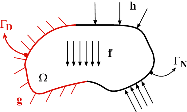
Figure 1: Sketch of a generic elastic body Ω subjected to volume forces f, to prescribed displacements g on a portion of the boundary Γ D, and to prescribed tractions h on the remaining portion Γ N

2.1 Primal Formulation

The primal (i.e., displacement-based) formulation of the small-strain linear elastostatic problem in strong form (Navier's equations) is given by

−∇⋅(C∇Su)=f,in Ω,(1)

complemented by the Dirichlet boundary conditions

u=g,on ΓD,(2)

and by the Neumann boundary conditions

(C∇Su)⋅n=h,on ΓN,(3)

where u(x) is the unknown displacement field (x being the position vector), ∇S is the symmetric part of the gradient operator ∇, n is the unit outward normal to the boundary of the domain, and C is the fourth-order elasticity tensor defined as follows:

C=2μI+λI⊗I,(4)

where I and I are the fourth- and second-order identity tensors, respectively, and λ and μ are the Lamé constants.

In this paper, the collocation approach is applied in the context of Isogeometric Analysis (IGA), and B-splines or NURBS [20] are used to represent both geometry and problem variables in an isoparametric fashion [21,22].

The basic ingredient for the construction of B-spline and NURBS basis functions is the knot vector, i.e., a set of non-decreasing coordinates in the parameter space: Ξ={ξ1=0,…,ξn+p+1=1}, where p is the degree of the B-spline and n is the number of basis functions. In the present work, we always employ so-called open knot vectors, where the first and the last knots have multiplicity p+1. Basis functions formed from open knot vectors are interpolatory at the ends of the parametric interval [0, 1] but are not, in general, interpolatory at interior knots.

The construction of the IGA collocation method is obtained following [6] by seeking an approximation uM for the unknown displacement field u of the elastic problem in the form

uM=∑i=1Mφ^i(G−1(x))u¯i,(5)

where φ^i, i=1,…,M, are the tensor-product B-spline basis functions which, following the isoparametric paradigm, are also used to represent the geometry of the problem. More precisely, we consider

{φ^1,…,φ^M}(6)

to be a set of basis functions defined on Ω^:=[0,1]d, d being the number of dimensions, such that the physical domain ω in (1) can be described by a global geometry function

G:Ω^→Ω¯,G(t):=∑i=1Mφ^i(t)ci,ci∈Rd,t∈Ω^,(7)

where ci∈Rd are the control points. We assume that the map G is a bijection. The unknown vectors u¯i∈Rd are referred to as displacement coefficients, or control variables. Expression (5) is substituted into Eqs. (1)–(3).

Let us assume for simplicity that d = 2. We denote by m1 and m2 the number of basis functions in the two parametric directions. Then M = m1m2 is the total number of unknown coefficients per displacement component. We choose M collocation points τkl, k={1,…,m1}, l={1,…,m2} located at the images of the tensor-product Greville abscissae of the knot vectors.1

The Greville abscissae [23] related to a univariate spline space of degree p and knot vector Ξ={ξ1=0,…,ξn+p+1} are points of the parametric space defined as

ξ¯i=ξi+1+ξi+2+…+ξi+pp.(8)

The Greville abscissae are simple to compute and have proven effective in many applications. However, there are other possibilities with interesting properties (e.g., [16,24]). In the two-dimensional primal case, 2M scalar equations are needed to determine the displacement coefficients. In the patch interior ω, we obtain 2(m1−2)(m2−2) scalar equations by collocating Eq. (1) at the points τkl, k={2,…,m1−1}, l={2,…,m2−1}:

[∇⋅(C∇SuM)+f](τkl)=0,τkl∈Ω.(9)

At the Dirichlet boundary ΓD we impose

uM(τkl)=g(τkl),τkl∈ΓD.(10)

To enforce Neumann boundary conditions, Eq. (3) is collocated at the points τkl∈ΓN according to the following strategy, see [7]:

[(C∇SuM)⋅n−h](τkl)=0,τkl∈edge⊂ΓN.(11)

[(C∇SuM)⋅nL−hL](τkl)+[(C∇SuM)⋅nR−hR](τkl)=0,τkl≡corner⊂ΓN,(12)

where nL and nR are the unit outward normals of the two edges meeting at the corner, and hL and hR are the respective imposed tractions. In addition, we refer the reader to [7] for a detailed discussion on the conditions to be imposed in more complicated situations, like at the interfaces of multi-patch geometries.

We note that, as has been shown in [13], the above “basic” approach to imposing Neumann boundary conditions may lead to difficulties in situations when non-uniform meshes are adopted. In such cases, alternative methods for imposing Neumann boundary conditions should be adopted, and in [13] two effective strategies are described.

2.2 Mixed u − p Formulation

A mixed u − p2 formulation is readily obtained starting from the equilibrium equations in differential form (1)–(3), written in terms of displacements, and introducing the “pressure-like” variable p = − λ ∇ ⋅ u, yielding:

{−μΔu−μ∇(∇⋅u)+∇p=f,in Ω,∇⋅u+p/λ=0,in Ω,(13)

complemented by the Dirichlet boundary conditions

u=g,on ΓD,(14)

and the Neumann boundary conditions

2μ∇Su⋅n−pn=h,on ΓN.(15)

We note that in the incompressible limit (λ → + ∞) p corresponds to the hydrostatic pressure. Otherwise, p is simply a scalar field defined by Eq. (13). See [1], Chapter 4, for elaboration. Despite this, in the remainder of the paper, we simply refer to p as the “pressure.”

In the mixed formulation we need to represent the pressure field in a similar, but not, in general, identical way as the displacement field. So we assume the pressure field takes the form

pN=∑i=1Nψ^i(G−1(x))pi.(16)

The pi are called the pressure coefficients, or pressure control variables, and the ψ^i are the corresponding B-spline or NURBS basis functions. Note, as per our assumption, in general, ψ^i are different than the φ^i basis functions of the displacement field. Expression (16) is now to be substituted into Eqs. (13) and (15).

Denoting by n1 and n2 the number of pressure basis functions in the two parametric directions, N = n1n2 is the total number of unknown coefficients for the pressure. We choose N collocation points τjhp, j={1,…,n1}, h={1,…,n2} located at the images of the tensor-product Greville abscissae of the knot vectors for the pressure field. In this case, 2M + N scalar equations are needed to determine the displacement and pressure coefficients.

In the patch interior Ω, we obtain 2(m1−2)(m2−2)+n1n2 scalar equations by collocating Eq. (13) at the points τklu, and τjhp, k={2,…,m1−1}, l={2,…,m2−1} and j={1,…,n1}, h={1,…,n2} as follows:

{[μΔuM+μ∇(∇⋅uM)−∇pN+f](τklu)=0,τklu∈Ω,[∇⋅uM+pN/λ](τjhp)=0,τjhp∈Ω.(17)

The Dirichlet and the Neumann boundaries are treated analogously to the primal case previously described. In particular, to enforce Neumann boundary conditions, Eq. (15) is collocated at the points τklu∈ΓN according to the following strategy:

[(2μ∇SuM)⋅n−pNn−h](τklu)=0,τklu∈edge⊂ΓN,(18)

[(2μ∇SuM)⋅nL−pNnL−hL](τklu)+[(2μ∇SuM)⋅nR−pNnR−hR](τklu)=0,τklu≡corner⊂ΓN.(19)

3  Numerical Results in 2D

The isogeometric collocation method is tested on two classical plane-strain elasticity problems: The first one entails homogeneous Dirichlet boundary conditions on the whole boundary, while the second one presents mixed Dirichlet and Neumann boundary conditions. Both benchmarks are implemented for an annular shape to include a non-trivial geometry map between the parametric and the physical domain.

For each problem we consider both compressible (λ/μ = 1) and nearly incompressible (λ/μ = 104) situations and we report convergence plots for all the unknown fields of the u − p formulation. After presenting the results obtained with the primal collocation formulation, clearly affected by locking in the nearly incompressible regime, the improvements produced by using the u − p collocation approach are shown. Unequal order approximations for the displacement and pressure fields are investigated. The polynomial order of the shape functions used for the displacement field is taken one order greater than that of the shape functions of the pressure field, i.e., we use QpQp − 1 elements. The idea is similar to the Taylor-Hood element of the Galerkin method. In that case both the displacement and pressure are C0-continuous. Here the displacement and pressure are Cp − 1-continuous and Cp − 2-continuous, respectively. Formulations of this type have been used successfully in isogeometric Galerkin methods, see [2,3].

In Fig. 2 the positions of the collocation points of the displacement and pressure fields are represented for the Q3Q2 case (m1 = m2 = 10, n1 = n2 = 9) for the quarter of annulus geometry considered in the following examples.

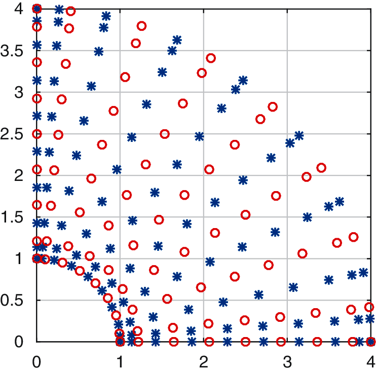
Figure 2: Position of the collocation points for the displacement field (blue stars) and pressure field (red circles) for the case of same meshes, Q3Q2 elements; number of displacement collocation points: m1 = m2 = 10, n1 = n2 = 9

Additionally, we compare the isogeometric collocation results obtained with finite element solutions obtained using a hybrid u-p formulation in Abaqus (Simulia, Dassault Systémes, Providence, USA), namely CPE4H elements, adopting piecewise bilinear displacement and constant pressure approximation. This element is a variant of the classical q1p0 element [4].

3.1 Quarter of an Annulus with Non-Uniform Body Load and Homogeneous Dirichlet Boundary Conditions

For the first benchmark, we refer to [6] and we consider a quarter of an annulus as sketched in Fig. 3, with an external radius Re = 4 and an internal radius Ri = 1.

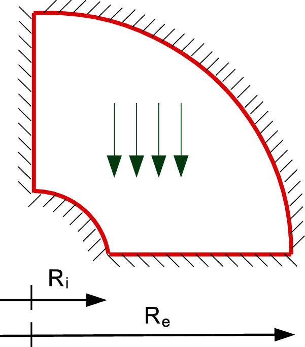
Figure 3: Quarter of an annulus with non-uniform body load and homogeneous boundary conditions

The domain is exactly represented by a single NURBS patch and is assumed to be clamped. Following [25], we assign a divergence-free manufactured solution in terms of displacement components, which satisfies the prescribed boundary conditions:

The load is then calculated starting from the manufactured solution.

3.1.1 Primal Formulation

In Fig. 4, we report for λ/μ = 1 and λ/μ = 104 the convergence plots of the L2-norm of the displacement error u * defined as

u∗=‖u1e−u1h‖2+‖u2e−u2h‖2‖u1e‖2+‖u2e‖2,(20)

where the superscript e stands for the exact displacement components, while the superscript h is used to indicate the components of the approximated displacement field. Primal pressures are derived from p = − λ (∇ ⋅ u). The exact pressures in this example are zero. Consequently, the pressure errors are reported as the absolute values.

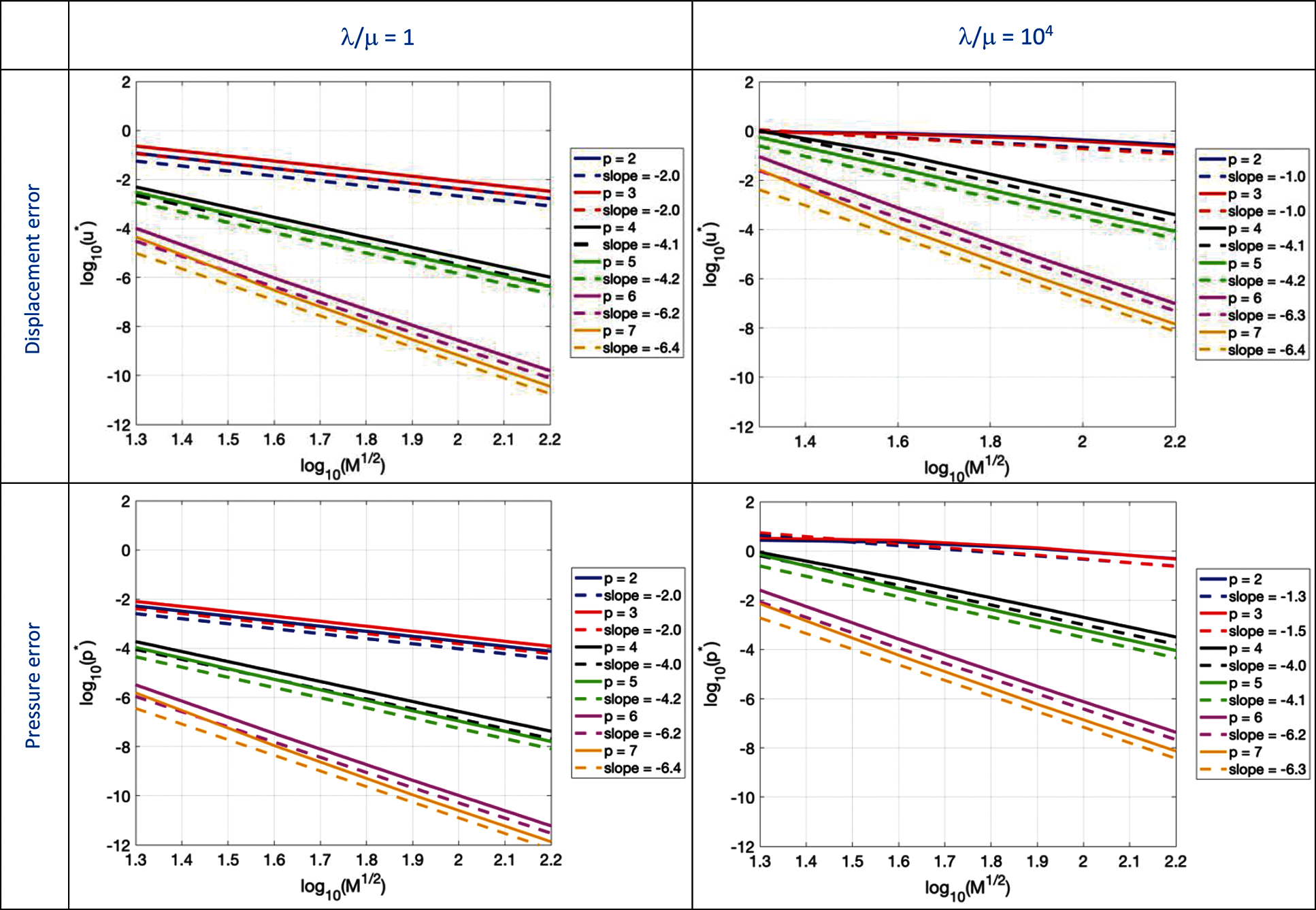
Figure 4: Primal formulation. Convergence plot of the L2-norm of the displacement and pressure error for the quarter of an annulus with non-uniform body load and homogeneous boundary conditions problem for λ/μ = 1 and λ/μ = 104

In Fig. 4, we also report the convergence plots of the L2-norm of the pressure error p*.

Remark. Throughout, convergence rates are determined from the two points of the convergence plots corresponding to the two finest meshes.

It is clear that, in the nearly incompressible regime, i.e., when λ/μ = 104, severe volumetric locking appears when using quadratic and cubic basis functions. For higher degrees (i.e., p > 3), the rates of convergence are the same as those obtained for λ/μ = 1, while the absolute errors are two to four orders of magnitude higher. The same observations can be made from Table 1 summarizing displacement and pressure error convergence rates and values.

3.1.2 Mixed u − p Formulation

The results obtained with the mixed u − p collocation method are reported in terms of convergence plots of the L2-norms of displacement and pressure errors in Fig. 5. Note that the exact solution for the pressure is pe = 0, therefore, for this example, p * cannot be normalized and represents the absolute error: p∗=‖pe−ph‖=‖ph‖ , that is the L2-norm of the numerical pressure.

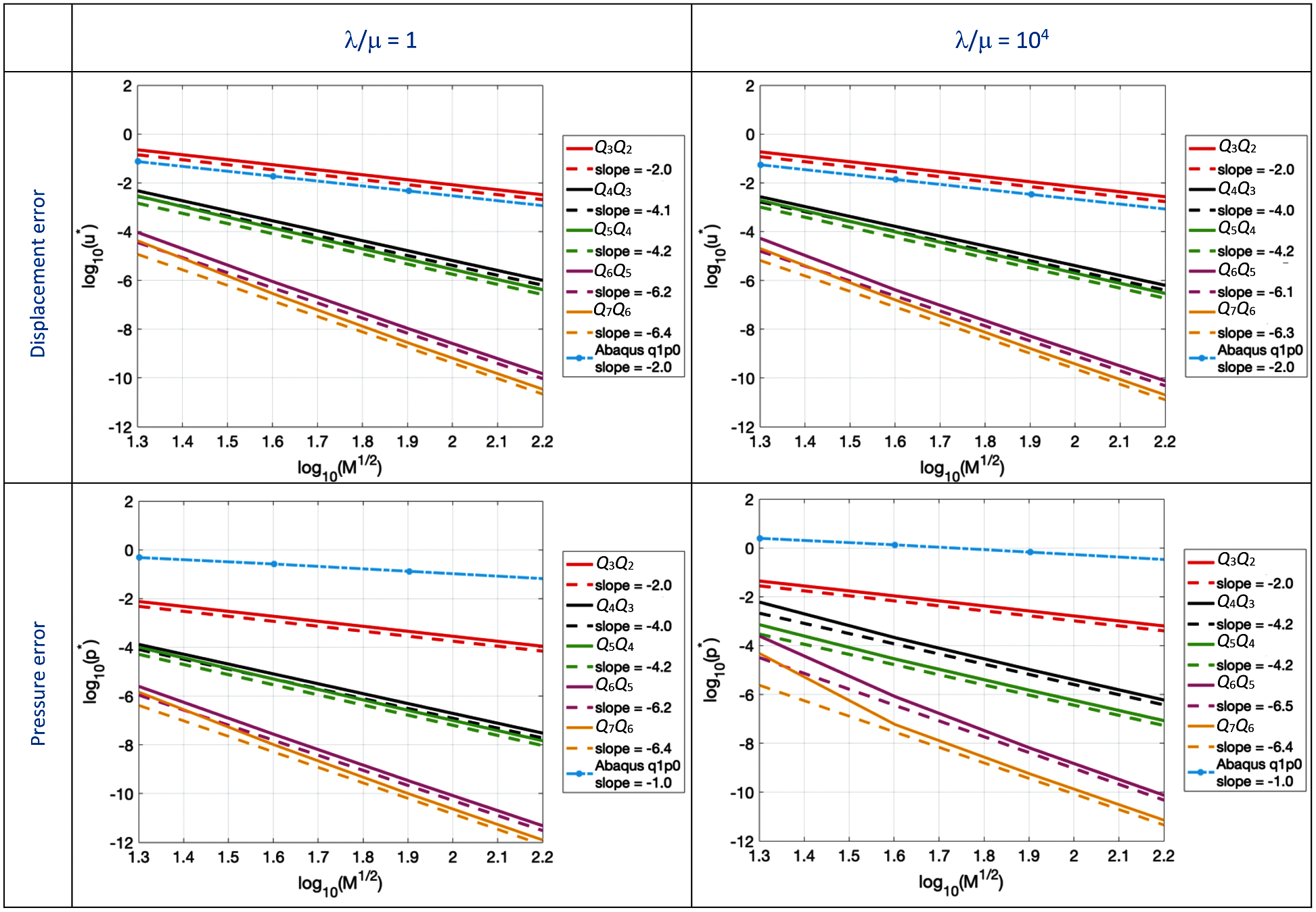
Figure 5: Mixed formulation (QpQp − 1). Convergence plot of the L2-norm of the displacement and pressure error for the quarter of an annulus with non-uniform body load and homogeneous boundary conditions problem for λ/μ = 1 and λ/μ = 104

Fig. 5 shows that no difference is observed in the displacement errors when moving from the compressible to the nearly incompressible regime. As also reported in Table 1, moving from λ/μ = 1 to λ/μ = 104, very similar error values are obtained using both coarse and fine meshes.

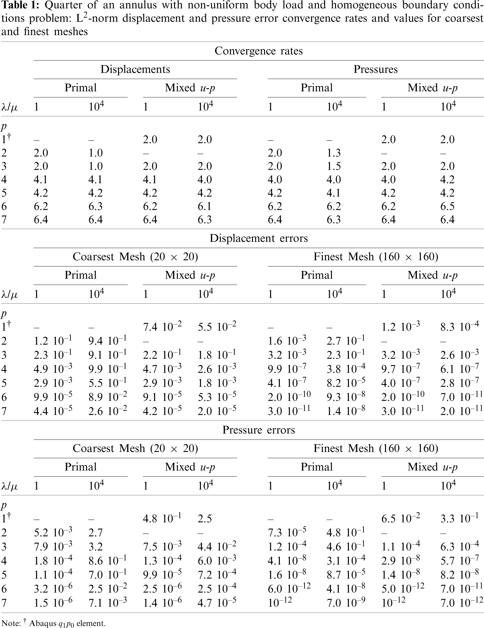
Fig. 5 also shows that, while the orders of convergence of the pressure error are not affected by the nearly incompressible regime, their values are higher. We may observe that the errors obtained by the Abaqus q1p0 element for displacements are comparable with those of the isogeometric collocation Q3Q2 case. However, the pressures of the Abaqus q1p0 element are substantially worse both in convergence rate and absolute values.

3.2 Infinitely Long, Pressurized Thick-Walled Cylinder

As a second example, we consider the infinitely long and internally pressurized thick-walled cylinder, studied in [6]. Exploiting the symmetry of the problem, we can consider only one quarter of the full domain, as represented in Fig. 6. As the cylinder is infinitely long, the problem can be solved as a two-dimensional plane strain problem. As in the previous example, we select an external radius Re = 4 and an internal radius Ri = 1.

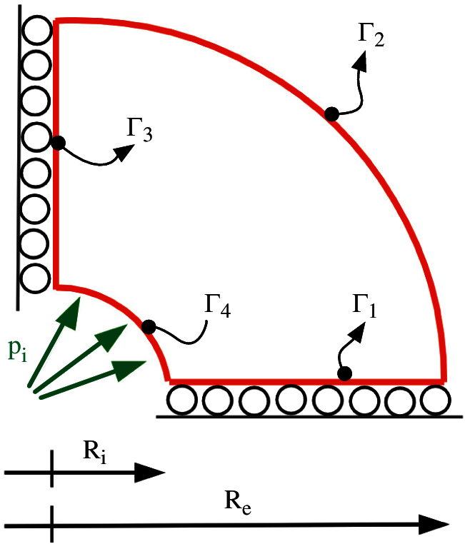
Figure 6: Infinitely long, pressurized thick-walled cylinder

The boundary conditions, depicted in Fig. 6, are

(σ⋅n)⋅τ=0andu2=0on Γ1σ⋅n=0on Γ2(σ⋅n)⋅τ=0andu1=0on Γ3(σ⋅n)⋅τ=0and(σ⋅n)⋅n=h¯ion Γ4,(21)

where τ is the unit tangent vector. The exact solution in terms of displacements (in radial and circumferential directions) is

ure=C1(h¯ir+C2r)uθe=0,(22)

where r indicates the radial position, C1=(1+ν)Re2Ri2E(Re2−Ri2), and C2=(1−2ν)h¯iRe2. The Young's modulus E and the Poisson's ratio ν are defined in terms of the Lamé constants as: E=μ(3λ+2μ)λ+μ and ν=λ2(λ+μ).

The aim of this test is to check whether mixed boundary conditions have an impact on the results.

Primal Formulation

The convergence plot of the L2-norm of the displacement error ur∗ defined as

ur∗=‖ure−urh‖2‖ure‖2,(23)

where ure and urh are the exact and approximate radial displacement components, respectively, is reported in Fig. 7 for λ/μ = 1 and λ/μ = 104, along with the convergence plot of the L2-norm of the pressure error p*, defined as

p∗=‖pe−ph‖2‖pe‖2,(24)

where pe and ph are the exact and approximate pressures, respectively. In the primal formulation case, pressures are derived from displacements.

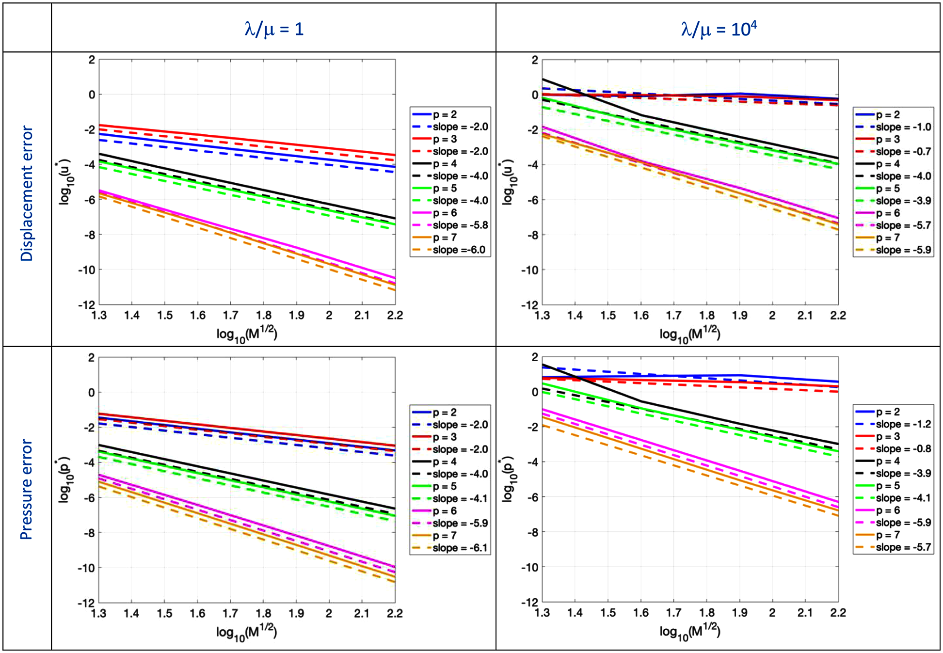
Figure 7: Primal. Convergence plot of the L2-norm of the displacement and pressure error for the infinitely long, pressurized thick-walled cylinder problem for λ/μ = 1 and λ/μ = 104

As expected, for the primal formulation, in the nearly incompressible regime, i.e., when λ/μ = 104, severe volumetric locking appears when using quadratic and cubic basis functions. When p is equal to 4, we observe that coarse meshes lead to significant errors and the obtained convergence rate is suboptimal both for displacements and pressures. For higher degrees (i.e., p > 4), the rates of convergence are the same as those obtained for λ/μ = 1, while the absolute errors are three orders of magnitude higher, as summarized by error values reported in Table 2.

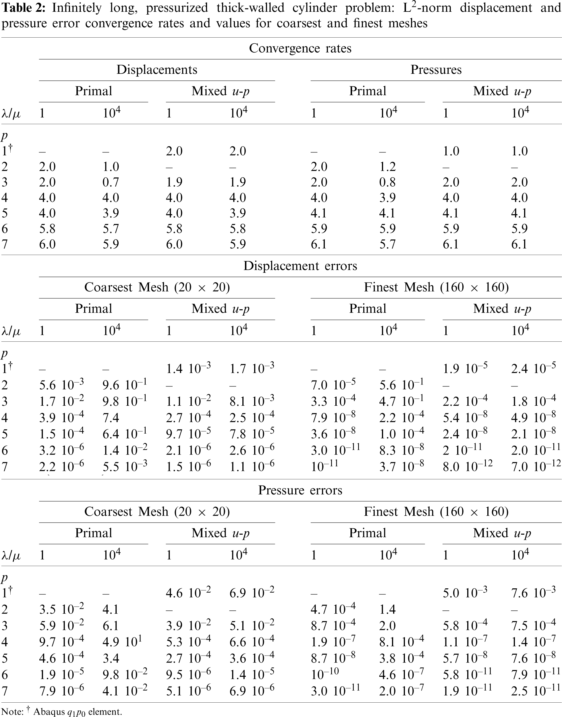
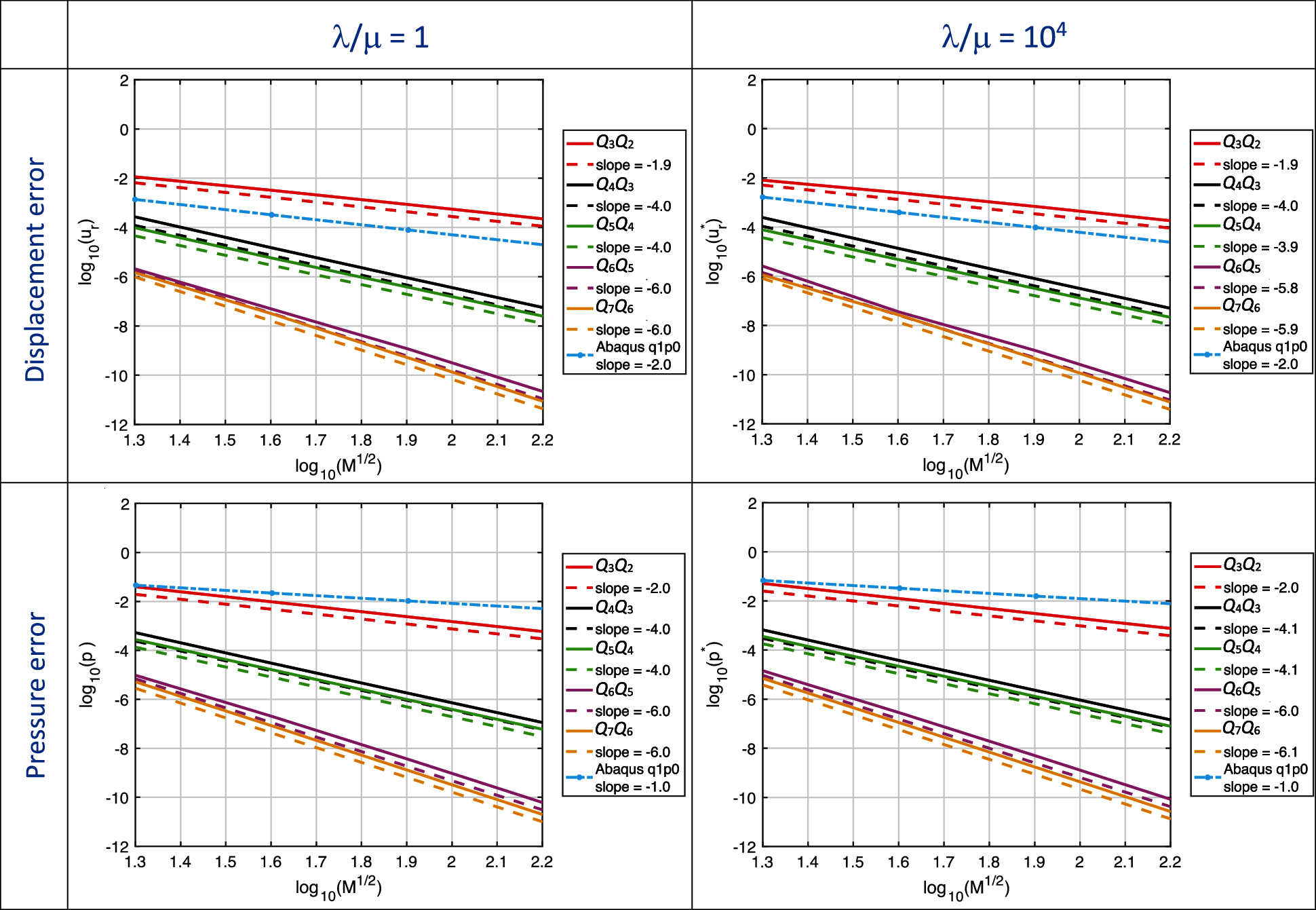
Figure 8: Mixed formulation (QpQp − 1). Convergence plot of the L2-norm of the displacement and pressure error for the infinitely long, pressurized thick-walled cylinder problem problem

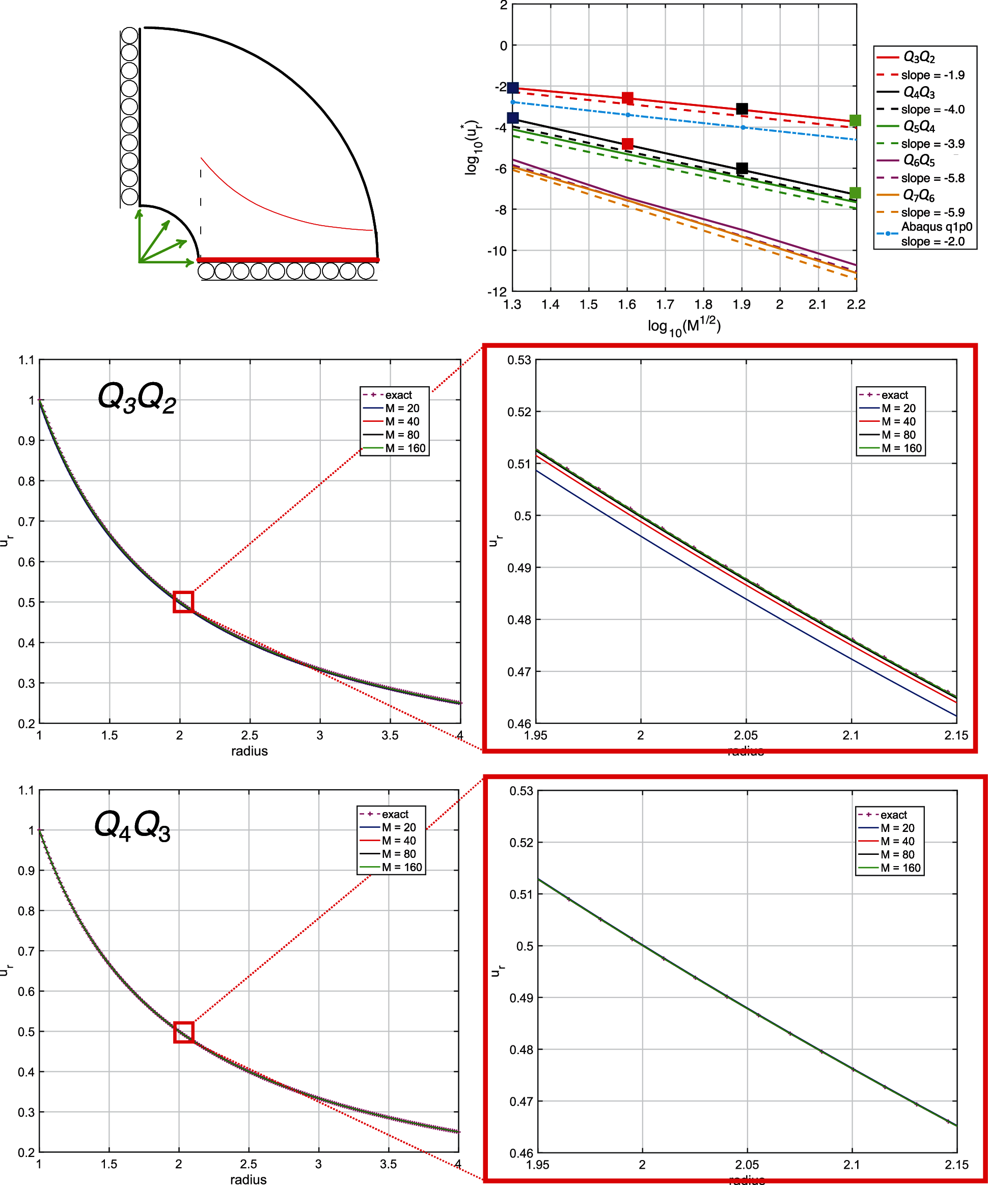
Figure 9: Line plots of displacement with different meshes vs. the radius for the case Q3Q2 and Q4Q3 (see square markers of the convergence plot in the top, λ/μ = 104)

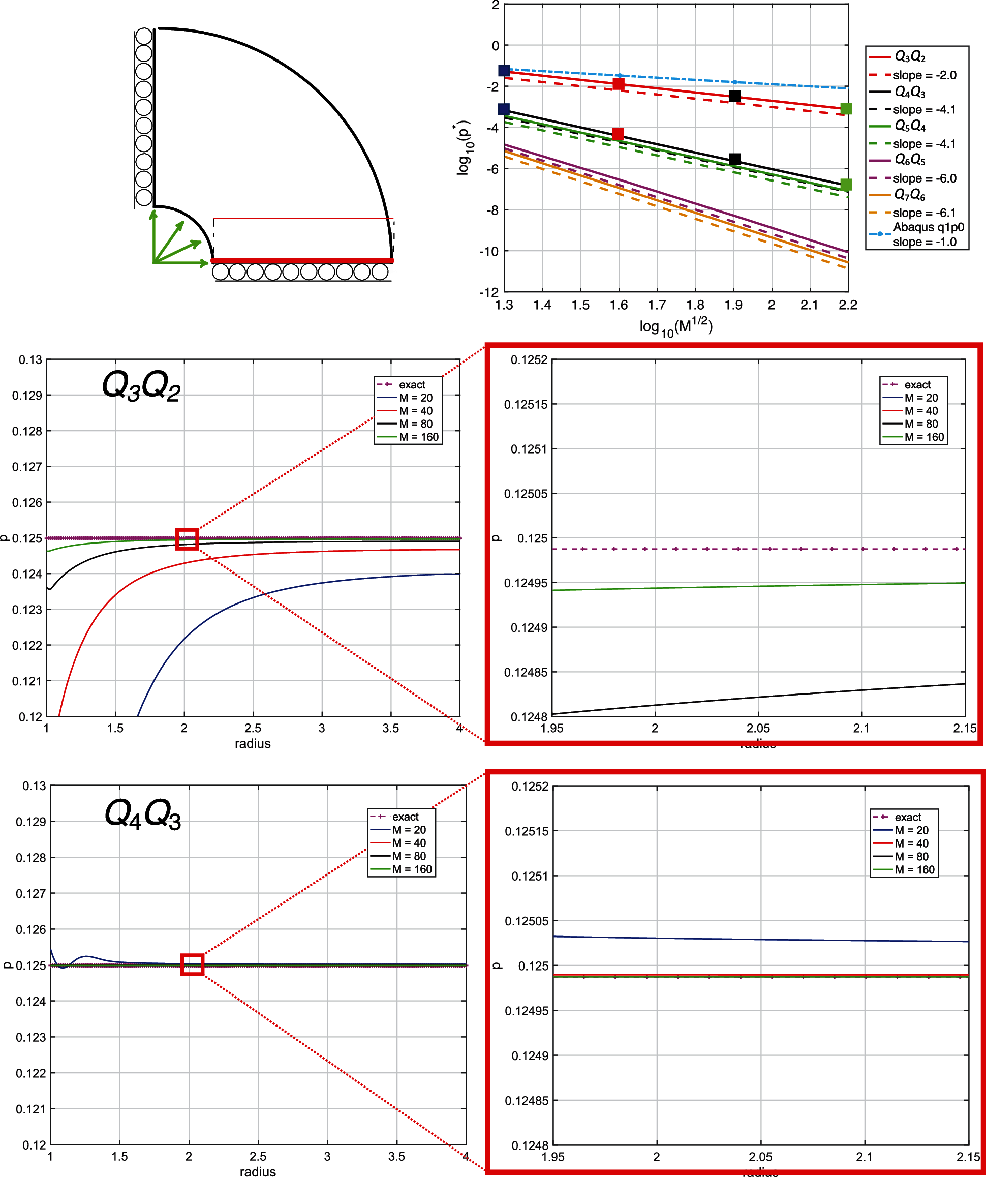
Figure 10: Line plots of pressure with different meshes vs. the radius for the case Q3Q2 and Q4Q3 (see square markers of the convergence plot in the top, λ/μ = 104)

3.2.2 Mixed u−p Formulation

The same trends observed in the previous benchmark are observed also in this case. In particular, optimal behavior in terms of both displacement and pressure errors is recovered in the nearly incompressible regime, as shown in Fig. 8. Both displacement and pressure errors listed in Table 2 are very similar when moving from λ/μ = 1 to λ/μ = 104. Displacement finite element errors (using again the Abaqus q1p0 element) are approximately one order of magnitude smaller than those obtained with isogeometric collocation with the Q3Q2 elements, but more than two orders of magnitude higher when p > 3. Pressure finite element errors are always greater than those obtained with collocation.

To better understand the performance of the u − p method in the nearly-incompressible regime, since everything varies only radially, line plots for the Q3Q2 and Q4Q3 cases of displacement and pressure results vs. the radius are reported in Figs. 9 and 10, respectively. While the radial displacement solution shows accurate results also for coarse meshes independent of the considered polynomial degree, the pressure results for the Q3Q2 case are less accurate for coarse meshes, but quickly improve under mesh refinement. Much improved pressure behavior is observed for the Q4Q3 case. For higher order cases there are no discernible errors on the scales of the plots for all meshes.

4  Numerical Results in 3D

We tested the u − p formulation on a 3D example and compared with Abaqus C3D8H elements, which are 8-node linear, hybrid, constant pressure elements. We again refer to this element as the q1p0 element. The considered solid depicted in Fig. 11 is characterized by the following dimensions: Ri = 1, Re = 4, H = 1, and is fully clamped on its entire boundary. We assign a manufactured solution in terms of displacement components, which satisfy the prescribed boundary conditions, which is not divergence free.

The load is then calculated starting from the manufactured solution and imposing equilibrium. We note that in the nearly-incompressible case the pressure loading will be amplified by a factor of 104. We remark that the results obtained behaved similarly to a 2D version of this problem, indicating that the dimension of the problem is not a significant influencer.

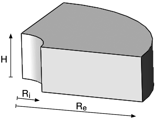
Figure 11: Three dimensional quarter of annulus

Primal formulation. In Fig. 12 the convergence plots of the L2-norm of the displacement3 and pressure error are shown for the primal formulation. As observed in the 2D examples, the displacement error exhibits locking for p = 2 and p = 3 when λ/μ = 104, while pressure seems to not be significantly affected by the nearly-incompressible constraint, as also shown by error convergence rates provided in Table 3. In comparison with the two 2D problems previously solved, the present results are qualitatively similar with respect to displacements, clearly manifesting locking in the nearly-incompressible case; however, the pressure results are quite different, indicating only slightly larger errors for the nearly-incompressible case compared with the compressible case, λ/μ = 1.

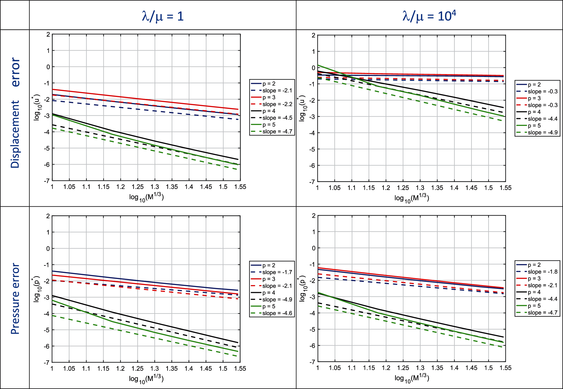
Figure 12: Primal formulation. Convergence plot of the L2-norm of the displacement and pressure error for the 3D quarter of an annulus with non-uniform body load and homogeneous Dirichlet boundary conditions problem for λ/μ = 1 and λ/μ = 104

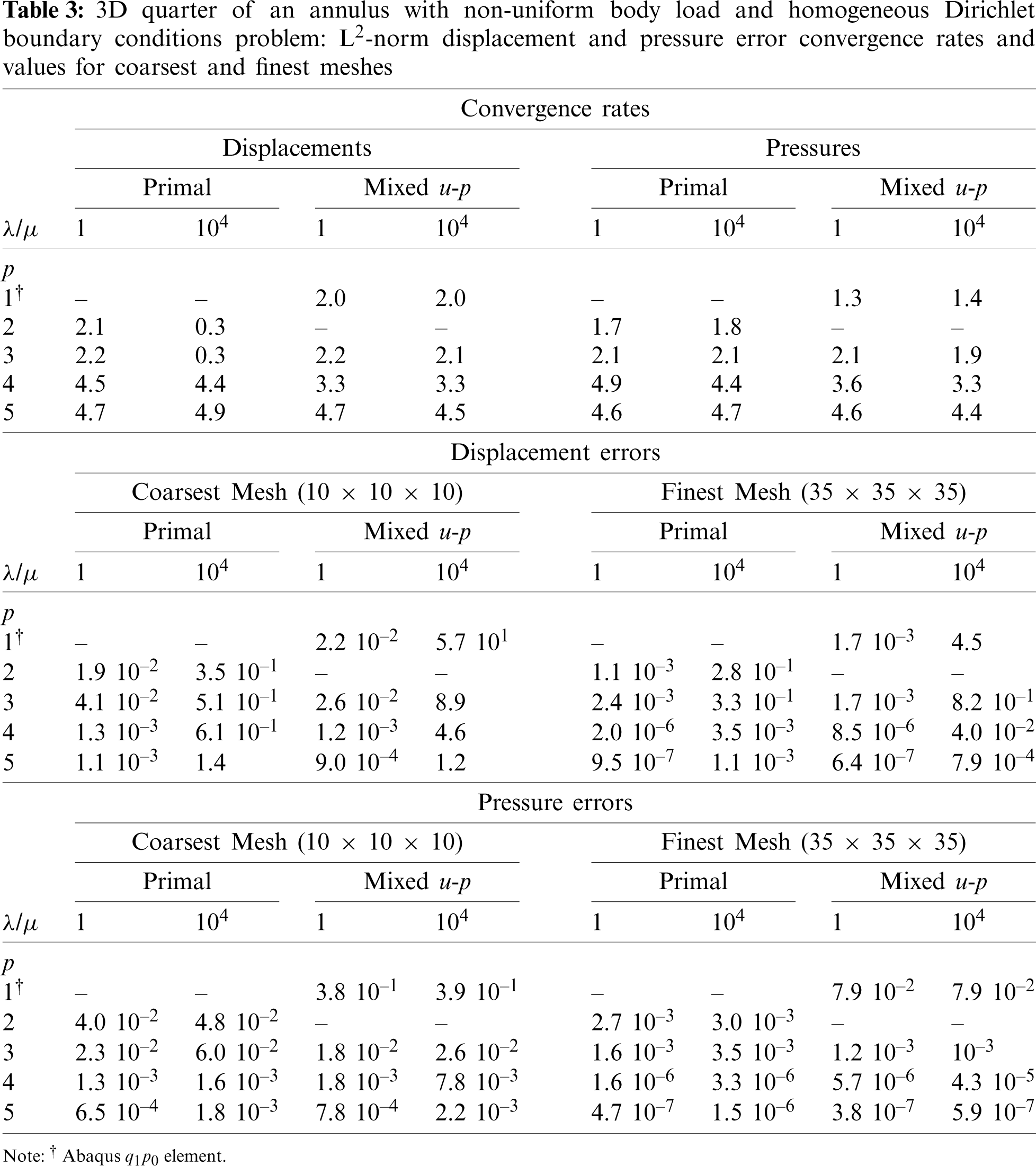
Mixed u-p formulation. In Fig. 13 the convergence plots of the L2-norm of the displacement and pressure error are shown for the mixed formulation. For the mixed collocation formulation, the displacement and pressure results for λ/μ = 1 are about the same as for the primal formulation, as reported in Table 3.

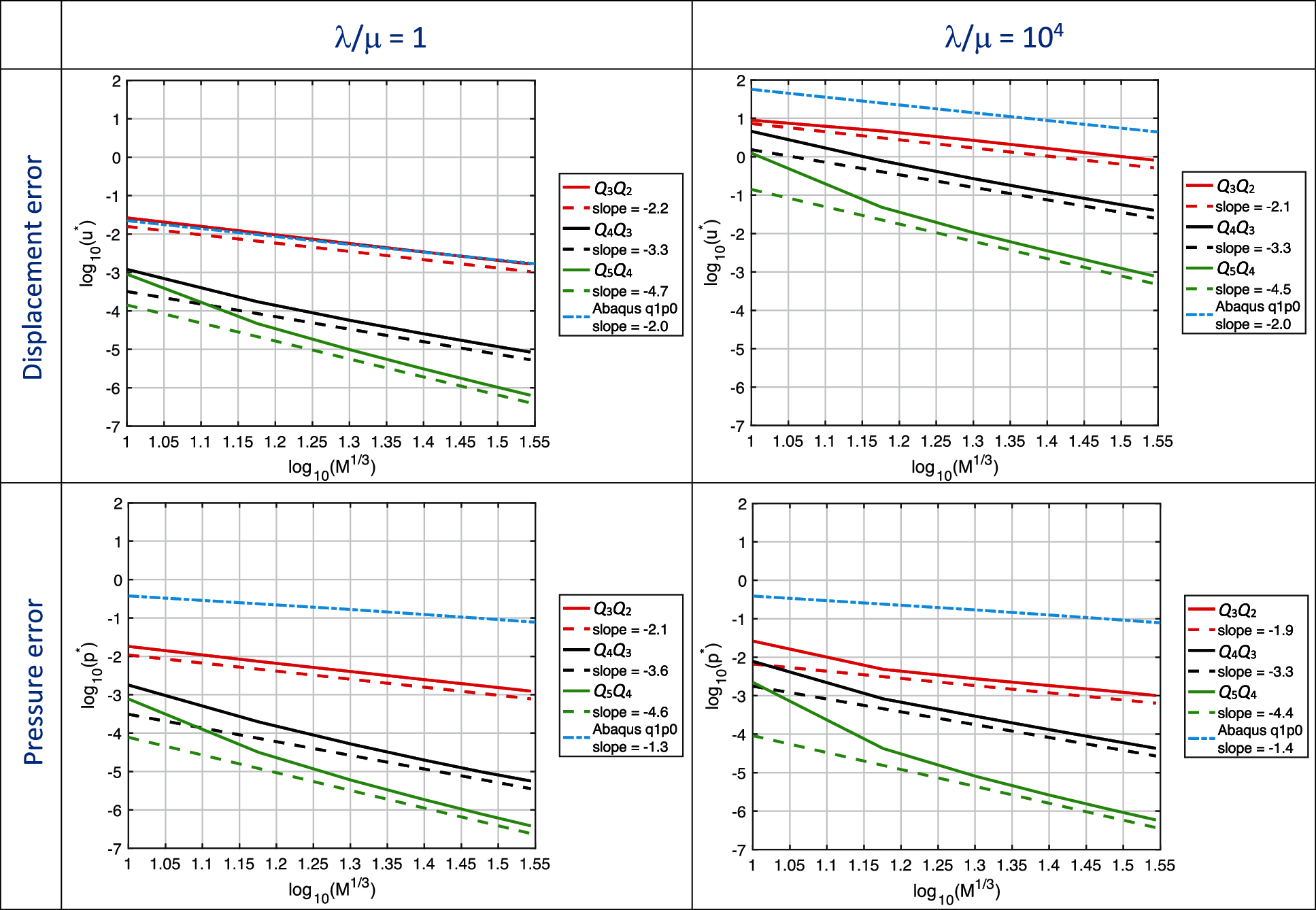
Figure 13: Mixed formulation (QpQp − 1). Convergence plot of the L2-norm of the displacement and pressure error for the 3D quarter of an annulus with non-uniform body load and homogeneous Dirichlet boundary conditions problem for λ/μ = 1 and λ/μ = 104

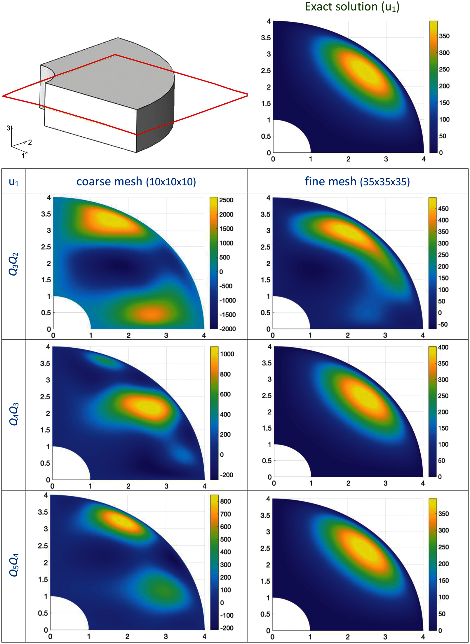
Figure 14: 3D quarter of an annulus with non-uniform body load and homogeneous Dirichlet boundary conditions problem: Surface plots of the first displacement component u1 for different orders and meshes (λ/μ = 104)

We note though that Abaqus q1p0 element produces substantially greater errors for pressure. For the case λ/μ = 104 the pressure results are all similar to those at λ/μ = 1. However, the displacement results at λ/μ = 104 are significantly in error and generally worse than for the primal formulation. This was not seen in either of the 2D cases presented earlier. As mention earlier, this behavior is not attributable to the problem being 3D as an analogous version of this problem in 2D behaved similarly. Surface plots obtained by cutting the domain with the plane highlighted in Fig. 14 are shown to better understand the u − p method results in the nearly incompressible regime. The first component of the displacement solution is shown. The left column of Fig. 14 highlights the inaccurate behavior of coarse meshes, while in the right column an improvement upon refinement is observed. Similar results are obtained for the other displacement components.

Normally, we are inclined to attribute inaccurate displacement results for the nearly-incompressible case to locking, but this does not seem to be what is occurring here, in fact, quite the opposite. Note the amplitude of the color bars in each frame and compare with that of the exact solution. The coarse and fine mesh results are converging toward exact from above. For the Q5Q4 case the results are visibly the same as exact and the color bar values are likewise the same as exact.

The coarse mesh results are enormously in error, both qualitatively and with respect to amplitude. For Q3Q2, the amplitude error is approximately one order of magnitude; the displacements are simply much too large, the antithesis of locking.

What is the explanation for the results of this problem? One might observe that the specification of the problem is somewhat contradictory. The material characterization is nearly-incompressible, indicated by the ratio of the Lamé parameters, λ/μ = 104. However, the manufactured solution does not respect this characterization in that its divergence is of the same order as its deviatoric component. The upshot is that the applied forces have a pressure component four orders of magnitude greater than the forces proportional to μ. It is clear from the large displacement response that those forces are being balanced partially by deviatoric deformations.

In addition to the unphysical nature of this problem we may point out that the results of the Abaqus q1p0 element are much the worst in error, both for displacements and pressure, and this element is widely used and considered appropriate for broad classes of real-world applications. However, we take the results of this problem to be cautionery, and indicative of the fact that both Galerkin and collocation results for mathematically well-posed problems may prove wanting in certain extreme cases. As a rule of thumb, it is clear that higher-order collocation results are significantly better than lower order, but even for higher order, sufficient mesh refinement of results is still necessary to obtain very accurate results.

We would now like to describe what we have seen from a mathematical point of view, termed “pressure robustness,” and thoroughly developed by Alexander Linke and his collaborators; see, e.g., (18) and references therein. Pressure robustness is an additional attribute to inf-sup stability asked of a discrete scheme by Linke. It can be stated for our problem as follows: part of the force scaled by λ is increased, holding μ fixed, the numerical displacement solution should be O(1), that is independent of λ. Our results clearly indicate this is not the case, and so we conclude none of the methods considered is pressure robust. In all cases they are O(λ) but perhaps mollified by some power of the mesh parameter h. Over the small range of meshes considered for this problem, 10 × 10 × 10 to 35 × 35 × 35, we might expect roughly three orders of magnitude deterioration of the solution with λ and this is the case. In the array of standard primal and mixed finite elements used in structural mechanics, the combination of inf-sup stability and pressure robustness is elusive. We note, however, that stabilized methods seem to alleviate this issue when most others fail, but their use in structural mechanics has been limited despite widespread use in fluids.

5  Conclusions and Summary of Results

In this paper we have investigated the behavior of isogeometric collocation methods in linear, isotropic elasticity with emphasis on the behavior in the nearly-incompressible case, taken as λ/μ = 104 herein, where λ and μ are the Lamé parameters. We also presented results for the compressible case, taken as λ/μ = 1 herein, for comparison. Two formulations of the problem were considered; the primal formulation utilizing the Navier equations of elasticity, and the mixed, displacement-pressure formulation. For the primal formulation we investigated NURBS based models of polynomial degree p=2,3,…,7. For the mixed elements, we considered displacement fields of degree p=3,4,…,7 and pressures one degree lower, a combination that has been shown to be effective previously in isogeometric Galerkin methods [2,3]. The primal formulation, when implemented in a standard, low-degree, Galerkin finite element method, is well known to suffer from displacement “locking.” The mixed formulation has been used to design both low- and high-degree finite elements that alleviate locking and have been successfully applied to engineering problems. The three numerical examples we considered herein asked similar questions of the isogeometric collocation methods. For context, we presented results for constant pressure Abaqus elements that are known not to lock and are widely used in engineering analysis.

A general statement about the results is that for the compressible case, there were no surprises. Both primal and mixed cases presented consistent convergence patterns, with higher-degree basis functions exhibiting greater accuracy.

For all problems studied, consistent patterns also emerged for the primal formulation. Locking was observed when λ/μ = 104 for p = 2 and 3. Higher-degree cases behaved better but the absolute values of displacement errors for the nearly-incompressible case were typically orders of magnitude higher than for the compressible case, despite convergence rates being the same. We conclude from these results that isogeometric collocation with the primal formulation is not effective for nearly-incompressible applications.

For the mixed formulation, applied to the two-dimensional problems, very good results were obtained in all cases. Even for the lowest degree case, Q3Q2, displacement errors were commensurate with the Abaqus q1p0 element in magnitude and exactly the same in rate of convergence, namely, O(h2); for pressures, the mixed collocation results were more accurate in magnitude and in rate, and again O(h2). The higher-degree cases were much more accurate. Convergence rates for both displacement and pressure were the same and of O(hp) and O(hp − 1), for even and odd numbered elements, respectively, and there was very little difference in error amplitudes for the nearly incompressible and compressible cases.

The three-dimensional problem presented a more complex story for the mixed method. The loading in this case had both λ- and μ-proportional terms, and the λ term dominated in the nearly-incompressible case. For the λ/μ = 1 case, all results behaved as expected. The pressure results did not degrade substantially for the λ/μ = 104 case compared with the λ/μ = 1 case. However, the displacement results were roughly three orders of magnitude worse in magnitude, although the rates of convergence were the same. It appears that the “constant” in the displacement error is order λ, perhaps mollified by a power of h. One might have initially assumed that this was due to locking, but scrutiny of the results indicated it was quite the opposite; the displacements were much too large. The explanation is as follows: The λ-proportional body force term is precisely a pressure gradient, but the discrete pressure-gradient term in the mixed methods failed to fully balance it. Part of the burden was shifted to the μ-term, thus producing displacements of order λ/μ.

The poor performance of mixed methods of the type studied here, when subjected to body forces that are gradients of a scalar, has been described as a lack of “pressure robustness” by Alexander Linke and collaborators [18]. Unfortunately, lack of pressure robustness is the rule rather than the exception and it seems to be at odds with most “inf-sup” stable methods. It has been suggested that “stabilized methods,” which accommodate any combination of displacement and pressure basis functions, in particular equal-order, might be able to alleviate stability and pressure robustness issues simultaneously, and we hope to investigate this in future work; see, e.g., Hughes et al. [26,27].

For all the problems studied, we presented corresponding results using Abaqus with q1p0 elements. These elements are widely used in practice and provide a benchmark for what may be considered acceptable in engineering applications. The results for the lowest-degree mixed collocation method, Q3Q2, were commensurate in accuracy with the q1p0 element for displacements, but considerably more accurate for pressures. The higher-degree mixed collocation methods were substantially more accurate for both, as might have been anticipated. We do not suggest this is an equitable comparison, but rather it serves as an indication that the mixed collocation methods achieve a level of accuracy that makes them viable for engineering computations.

1In the three-dimensional setting (d = 3), we proceed in a completely analogous way, considering the third parametric direction (e.g., the M = m1m2m3 collocation points will be indicated as 'τklm, with k = {1, …, m1}, l = {1, …, m2}, m = {1, …, m3}).

2Throughout, the most popular symbols for both spline degree and pressure are used, namely p; The differentiation between the two is made clear by the context.

3The L2-norm of the displacement error u * is now defined as (25)u∗=‖u1e−u1h‖2+‖u2e−u2h‖2+‖u3e−u3h‖2‖u1e‖2+‖u2e‖2+‖u3e‖2, where u1e, u2e, and u3e are the exact displacement components, while u1h, u2h, and u3h are the approximated displacement ones.

Funding Statement: FF and LDL gratefully acknowledge the financial support of the German Research Foundation (DFG) within the DFG Priority Program SPP 1748 “Reliable Simulation Techniques in Solid Mechanics”. AR has been partially supported by the MIUR-PRIN project XFAST-SIMS (No. 20173C478 N).

Conflicts of Interest: The authors declare that they have no conflicts of interest to report regarding the present study.

This work is licensed under a Creative Commons Attribution 4.0 International License, which permits unrestricted use, distribution, and reproduction in any medium, provided the original work is properly cited.