| Computer Modeling in Engineering & Sciences |
DOI: 10.32604/cmes.2021.016851
ARTICLE
Virtual Element Formulation for Finite Strain Elastodynamics
Dedicated to Professor Karl Stark Pister for his 95th birthday
Institute for Continuum Mechanics, Leibniz Universität Hannover, Hannover, 30419, Germany
*Corresponding Author: Peter Wriggers. Email: Wriggers@ikm.uni-hannover.de
Received: 1 April 2021; Accepted: 12 May 2021
Abstract: The virtual element method (VEM) can be seen as an extension of the classical finite element method (FEM) based on Galerkin projection. It allows meshes with highly irregular shaped elements, including concave shapes. So far the virtual element method has been applied to various engineering problems such as elasto-plasticity, multiphysics, damage and fracture mechanics. This work focuses on the extension of the virtual element method to efficient modeling of nonlinear elasto-dynamics undergoing large deformations. Within this framework, we employ low-order ansatz functions in two and three dimensions for elements that can have arbitrary polygonal shape. The formulations considered in this contribution are based on minimization of potential function for both the static and the dynamic behavior. Generally the construction of a virtual element is based on a projection part and a stabilization part. While the stiffness matrix needs a suitable stabilization, the mass matrix can be calculated using only the projection part. For the implicit time integration scheme, Newmark-Method is used. To show the performance of the method, various two- and three-dimensional numerical examples in are presented.
Keywords: Virtual element method; three-dimensional; dynamics; finite strains
The virtual element method (VEM) can be seen as an extension of the classical finite element method (FEM) based on Galerkin projection. It allows meshes with highly irregular shaped elements, including concave shapes, as outlined in [1]. This gives more flexibility and new possibilities to geometry discretization in solid- and fluid-mechanics. The large number of positive properties of VEM increases the variety of possible applications in engineering and science. Recent works on virtual elements have been devoted to linear elastic deformations in [2–4], contact problems in [5], elasto-plastic deformations in [6–8], anisotropic materials in [9–11], curvilinear virtual elements for 2D solid mechanics applications in [12], hyperelastic materials at finite deformations in [13,14], crack-propagation for 2D elastic solids at small strains in [15] and phase-field modeling of fracture in [16,17].
Despite the fact that dynamic behavior has a strong influence on the mechanical properties and the prediction of their real response, most of the investigations introduced above are only done for static problems so far. In this regard, Park et al. [18] proposed a virtual element method for linear elastodynamics problems which is restricted to small strains. This has motivated the presented contribution in which we extend the application of VEM from the static to the dynamic case in the finite deformation range. Damping effects will not be considered in this investigation.
Typically the construction of a virtual element is divided into a projection part and a stabilization part. Within the projection part, a quantity
The structure of the presented work is as follows. In Section 2 the governing equations for nonlinear elastodynamics are outlined. Section 3 summarizes the virtual element formulation. Section 4 includes details on the computation of the element mass matrix. To verify the proposed virtual element formulations, various examples are demonstrated and discussed in Section 5. Section 6 briefly summarizes the work and gives some concluding remarks.
2 Governing Equations for Nonlinear Elastodynamics
In this section we summarize the finite strain elasto-static formulation (see e.g., [25 –27]) and supplement it by the dynamic effect. For that consider an elastic Body
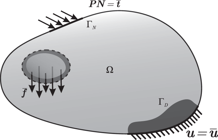
Figure 1: Solid with boundary conditions
The position
where
where the gradient is evaluated with respect to the initial configuration
The solid
where
here
where
in terms of the bulk
With the above set of equations, the finite strain elastodynamic problem is well formulated. Next, we use the potential function as a starting point for the development of a discretization method1. The static part of the potential is defined as
Generally it would be necessary to start from a Hamiltonian to obtain a potential form in elastodynamics. However for the purpose of generating residuals and tangents it is sufficient to formulate a dynamic pseudo potential that describes inertial effects
and to keep the inertia term
The total potential is then defined as the sum of static and inertia parts
3 Formulation of the Virtual Element Method
The main idea of the virtual element method is to use a Galerkin projection, which maps the primary fields (displacements in this work) to a specific polynomial ansatz space. Thus, the domain
In general, for finite strains the deformation map
The central concept of the virtual element method relies on the split of the ansatz space
For a linear ansatz, the projection
where
Furthermore, the projection
where
The strain energy function depends only on the gradient of the projection
Applying divergence theorem to (14) yields
at the element level. Here
By employing the linear ansatz space, the left hand side of (15) takes the simple form
In the 2D case, the right hand side of (15) is evaluated along the edges. As the displacements are known at the boundary, which are straight line segments, a linear ansatz for the displacements is used, see [14]. However, in the 3D case, the element boundary consists of polygonal faces. Therefore the evaluation of the integral in (15) is not straight forward, unless an appropriate ansatz is found. For the evaluation, there are two possible methods available. The first one is presented in [3], where the faces are subdivided in quadrilateral elements where the corners of the quadrilateral elements have certain positions. Finally the evaluation of the integral is carried out on those quadrilateral elements. An alternative option is to subdivide the element faces into 3 noded triangles. The integration is then carried out over the triangles of the polygonal faces by using the standard ansatz function for a linear triangle and Gauss integration:
as outlined in [6]. Here
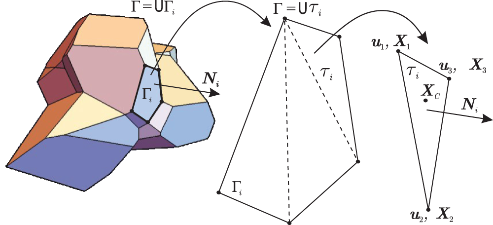
Figure 2: Virtual element faces split into multiple triangles
Here nf is the number of element faces.
All quantities are related to the initial configuration. Comparing (16) and (19), the unknown virtual parameters
The constant part of the projection
where nV is the total number of boundary nodes and
Finally with Eqs. (15) and (24) the ansatz function
where
For the time integration scheme, we use the implicit Newmark method outlined in [23,24]. The equations for the velocity
where
3.3 Construction of the Virtual Element
As introduced in Section 3.1, the formulation of a virtual element undergoing large deformations is based on a split of the energy into a constant part and an associated stabilization term. The nodal degrees of freedom of an element are in each element projected to a polynomial projection function. Further each displacement component is approximated with the same interpolation function, but having unique set of

For the consistency part, the projection
The gradient of the projection
which is still nonlinear with respect to the unknown nodal degrees of freedom.
The acceleration can be evaluated from (28) as
1. First possibility is to evaluate the integral at the centroid
2. Another possibility is to introduce a sub-triangulation of the polygon or polyhedra and again use one point Gauss integration which yields an evaluation at the integration points
Since the integral contains quadratic terms of X, Y and in 3D additionally of Z, the integration above approximates the integral.
3. As a third option, the integral can be exactly computed using the nodal coordinates at the boundary via divergence theorem, see [29,30]
The consistency term is computable but yields to a rank deficient stiffness matrix and thus needs to be stabilized. The idea is to introduce a new positive definite energy
We further define a stabilization parameter
Here,
Applying Eq. (38) in Eq. (29) yields the final form of the total potential energy function

For the case where

The consistency part in Eq. (40) can be computed in a similar way as described in Section 3.3.1. The stabilization part needs an approximation, see e.g., [14]. The displacement field is approximated by introducing an internal submesh of 3 noded triangles in 2D or 4 noded tetrahedra in 3D with linear ansatz functions
where
The stabilization parameter
4 Solution Scheme and Linearization
A global Newton type iteration results to the following linearized system of equations:

which allows to determine at given global primary field of unknowns
To obtain the element residual vector
Note that
With (25) we can write for the projected displacement, velocity and acceleration
and equivalently for the ansatz
Inserting Eq. (48) into Udyn in (30) and using the procedure in (47) yieds the explicit form of the residual for the Newmark time integration with Eqs. (27) and (28) for the projected part
with
with
The projection and stabilization part of the total element tangent for the dynamic part takes the form, note that differentiation is only performed with respect to nodal displacements at time tn+1
The total element tangent includes static and dynamics parts of the projection and stabilization
All differentiations leading to the residual and tangent of the elastodynamic virtual element were obtained with the software tool AceGen, see [26]. It provides the most efficient element routines when a potential formulation is used. Let us note that the exact weak form (6) follows from Ustat and from the pseudo potential Udyn for fixed accelerations and thus the derivation above is equivalent to using the weak form directly. With expressions (27), (28), (47) and (53) at hand the global tangent matrix
It is sufficient to use the consistency term alone (i.e.,
The presented tangent matrix
In this section we demonstrate the performance of the derived 2D and 3D virtual element formulation for dynamic problems at finite deformations. For comparison purposes results of the standard finite element method (FEM) are included. The material parameters used in this work are the same for all examples and provided in Table 1.
In this contribution, the following mesh types with first order virtual element discretizations are introduced. Different ways to evaluate the mass matrix
• VEM
— Q1: A regular 2D mesh with 4 noded quadrilateral elements.
— Q2S: A regular 2D mesh with 8 noded quadrilateral elements.
— VO: 2D/3D Voronoi cell mesh with arbitrary number of element nodes.
— H1: A regular 3D mesh with 8 noded hexahedral elements.
— H2S: A regular 3D mesh with 20 noded hexahedral elements.
• VEM
• VEM
• VEM
• VEM
For a representative comparison, the following finite element formulations were selected:
• FEM T1: A regular 2D mesh with 3 noded triangular first order finite elements.
• FEM Q1: A regular 2D mesh with 4 noded quadliteral first order finite elements.
• FEM Q2: A regular 2D mesh with 9 noded quadliteral second order finite elements.
• FEM H1: A regular 3D mesh with 8 noded first order finite elements.
• FEM H2: A regular 3D mesh with 27 noded second order finite elements.
For all the simulations the stabilization parameter of the static part was chosen as
In this section, the eigenfrequencies of a single element and of a structural system are analyzed to check the correctness of the eigenmodes and the eigenfrequencies when compared to classical finite elements.
The eigenfrequencies of a single quadliteral element which has a free-free boundary condition are shown in Table 2. Here eigenfrequencies related to rigid body motions are excluded. To investigate the effect of the stabilization parameters
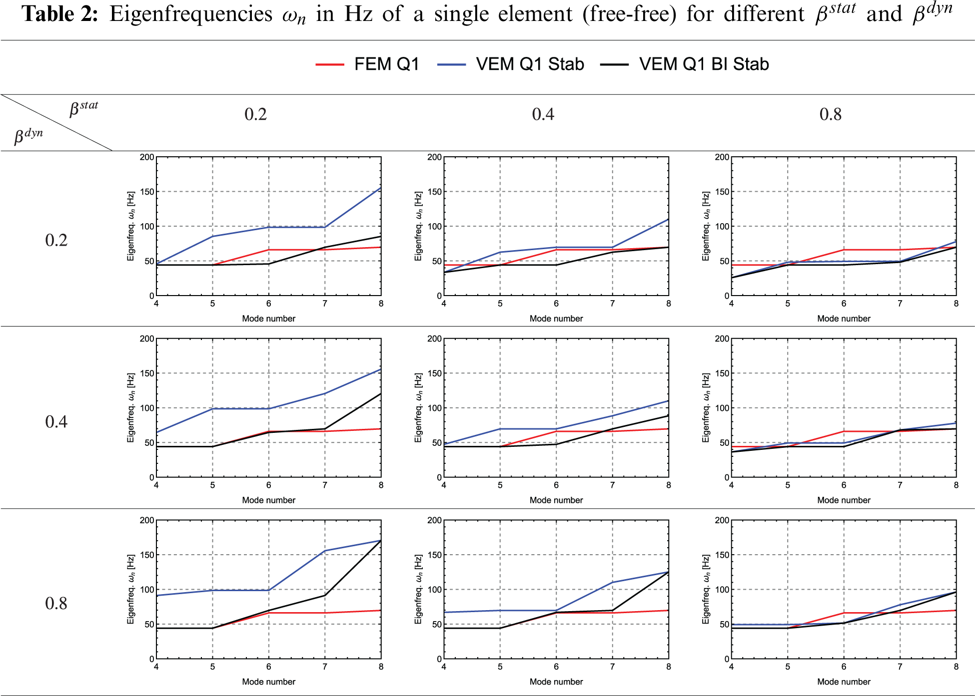
For
The standard finite element FEM Q1 in Fig. 3a.
— The virtual element VEM Q1 Stab in Fig. 3b, evaluating the dyamic part with Eq. (32).
— The virtual element VEM Q1 BI Stab in Fig. 3c, evaluating the dynamic part with Eq. (35).
— The virtual element VEM Q1-I Stab in Fig. 3d, evaluating the dynamic part with Eq. (33), using the submesh.
— Note that all these virtual elements have a stabilized mass matrix, since the computation of eigenfrequencies with rank deficient mass matrix is not possible for a single element.
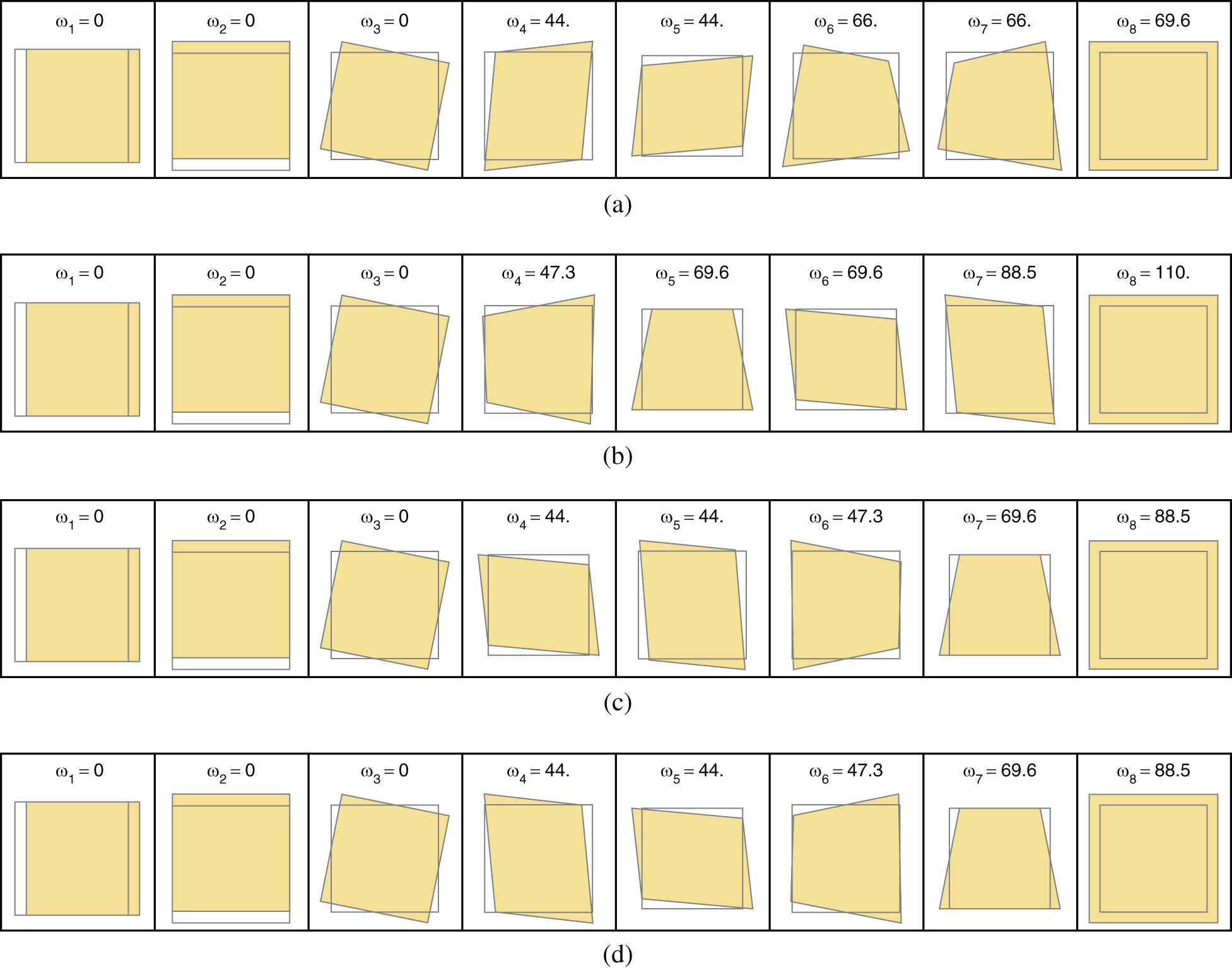
Figure 3: Eigenfrequencies
An eigenvalue analysis of the mass and stiffness matrix for the computation of specific initial boundary value problems is performed. A cantilever beam, which is clamped at one side and free at the other side (C-F) is considered. The material parameters are taken from Table 1. The beam has a length
Fig. 4 shows the eigenvalues with respect to the mode numbers, obtained with FEM Q1 and VEM Q1 Stab. In all figures no distinction is made between the mode types. The eigenvalues are computed with a discretization that has 360 unknowns. The eigenvalues of the stiffness and mass matrix computed with VEM are very close to the eigenvalues obtained by FEM. Note that a mass matrix which is based purely on the projection part (
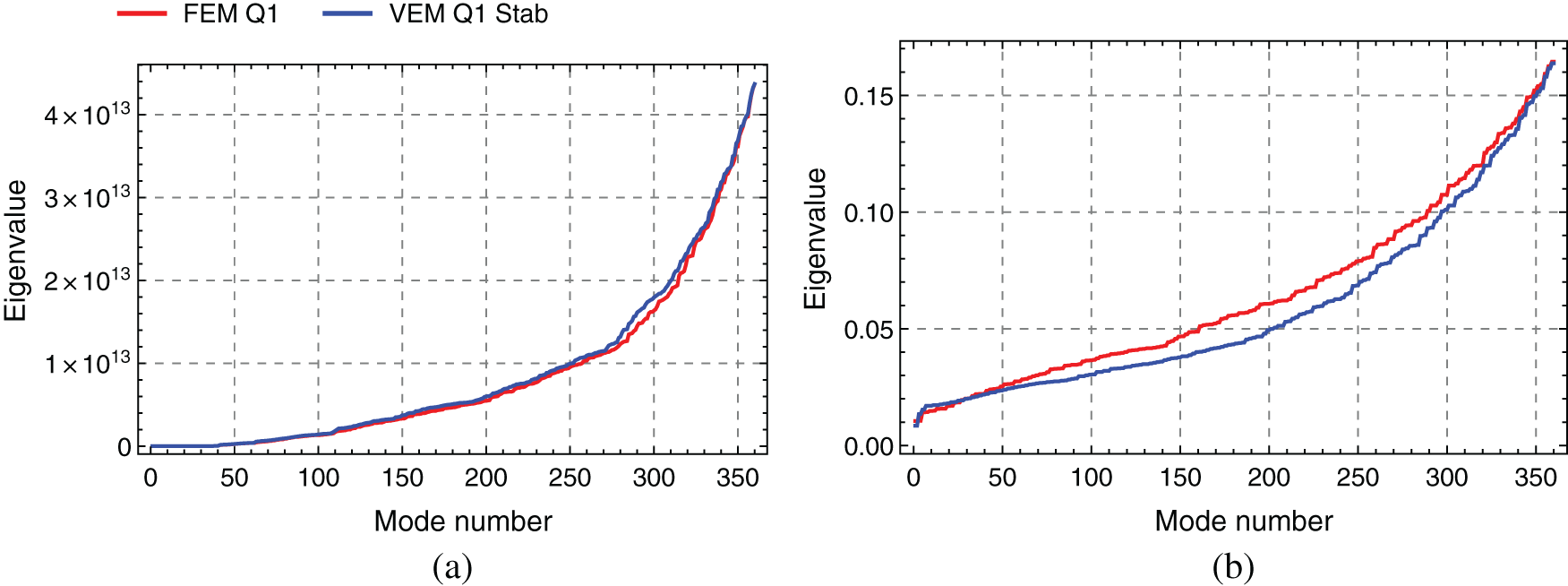
Figure 4: Eigenvalues of stiffness and mass matrix for 2D beam (C-F) (a) Eigenvalues of stiffness matrix
Table 3 depicts the eigenfrequencies which are corresponding to the first six longitudinal (L) and transversal (T) modes for two different mesh densities. For the longitudinal modes, the eigenfrequencies computed with VEM Q1 Stab are nearly the same when compared to the eigenfrequencies obtained with FEM Q1 (see also Fig. 5). For the bending modes, the eigenfrequencies have some shift, but they are in a good agreement. However, when increasing the number of nodes, changing the element topology from Q1 to Q2S topology (from 4 to 8 nodes per virtual element), the quality of the computed eigenfrequencies increases for the virtual element. We note that the eigenvalues are converging to the analytical solution for all element types for refined meshes.
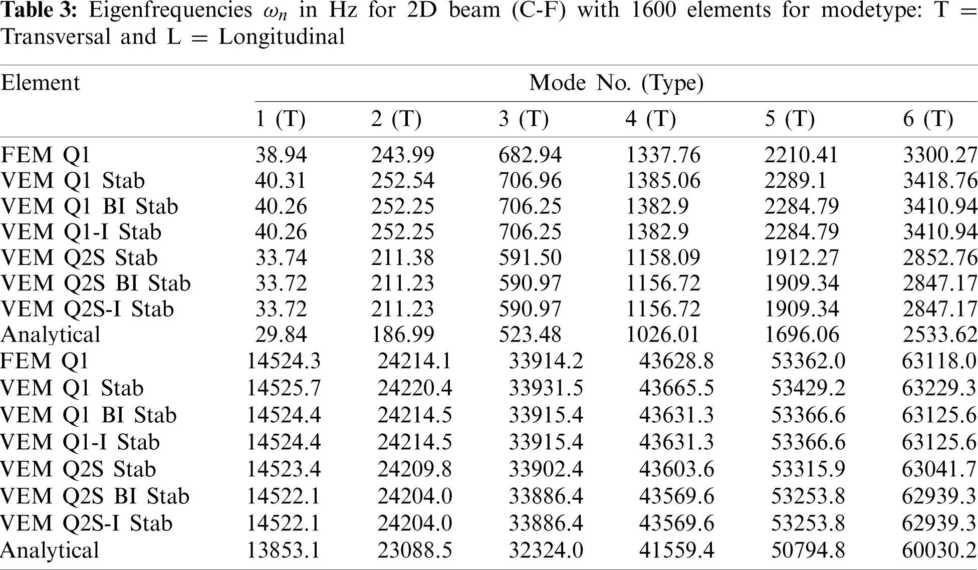
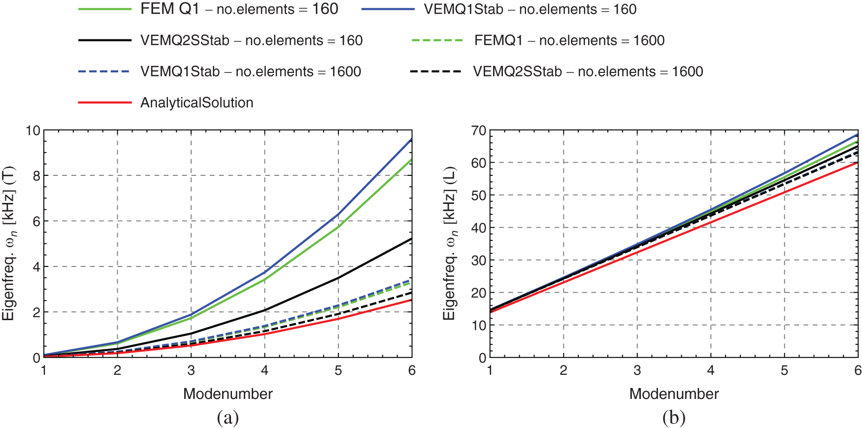
Figure 5: Eigenfrequencies for 2D beam (C-F) (a) Eigenfrequencies of transversal modes (b) Eigenfrequencies of longitudinal modes
5.2 2D Boundary Value Problems
5.2.1 Wave Propagation in Longitudinal Beams
In this example wave propagation in longitudinal beams is analyzed. The geometric setup and the loading conditions of the specimen are depicted in Fig. 6. Table 1 provides the material parameters. The height of the beam is chosen to be
For both virtual elements VEM Q2S and VEM Q2S Stab the integral for the dynamic part in Eq. (30) is evaluated at the centroid of the element, hence this simple and efficient scheme seems to be sufficient.
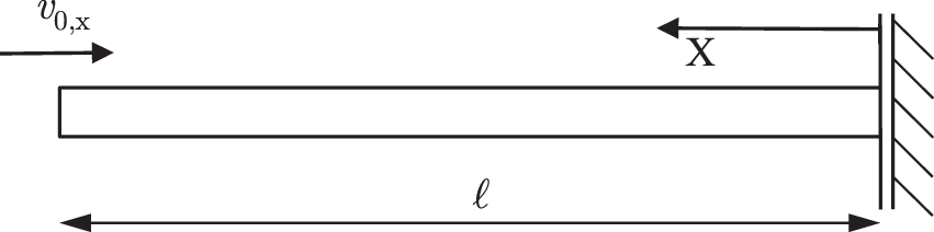
Figure 6: 2D example–-Wave propagation in longitudinal beams (boundary value problem)
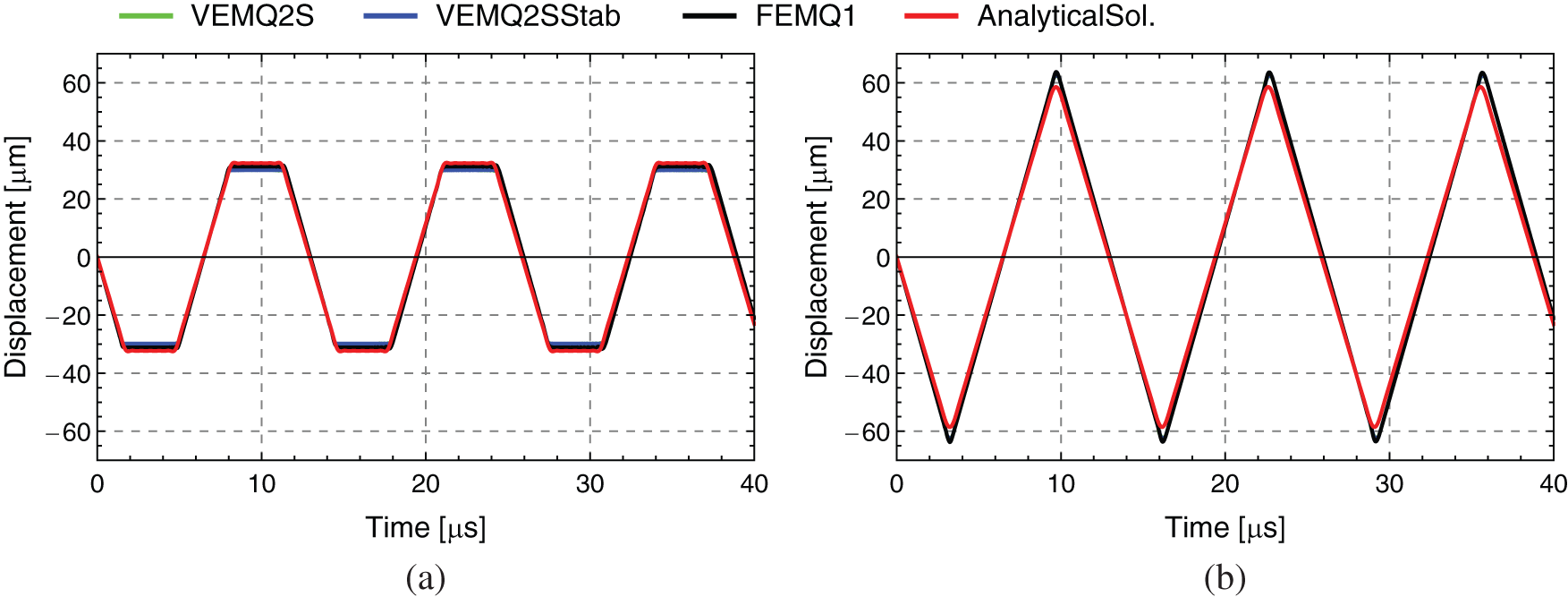
Figure 7: Displacement over time response for 2D example–-Wave propagation in longitudinal beams (a) Response at
5.2.2 Transversal Beam Vibration
The second benchmark test is concerned with the analysis of transversal vibrations in beams. The geometric setup and the loading conditions of the cantilever beam are depicted in Fig. 8a. For the material parameters see Table 1. The length of the bar is set to
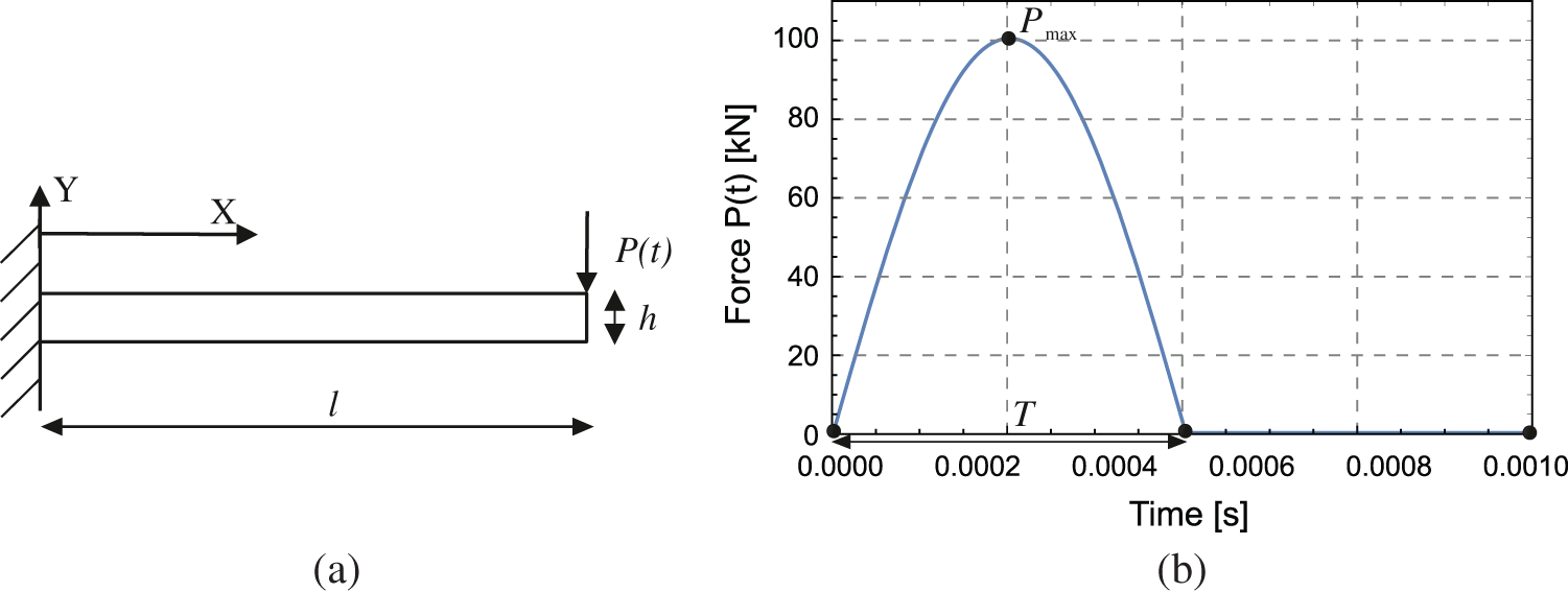
Figure 8: 2D example–-Transversal beam vibration. Boundary value problem in (a) and applied force in (b)
In order to analyze the position effect of the element centroid on evaluating the integral of the dynamic part, we used different type of meshes which can be seen in Fig. 9. The “animal” mesh (Fig. 9b) includes concave elements. To see the effect of using concave elements where the centroid of the element is outside of the element domain, we use a special mesh with elements like C’s, where the centroid of the element is outside of the element domain (Fig. 9c).
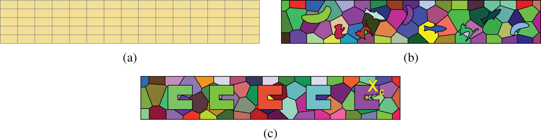
Figure 9: 2D example–-Transversal beam vibration. VEM Q2S Mesh (a), VEM Animal-Mesh (b) and C-Mesh (c)
Figs. 10 and 11 show the displacement over time response in the center at
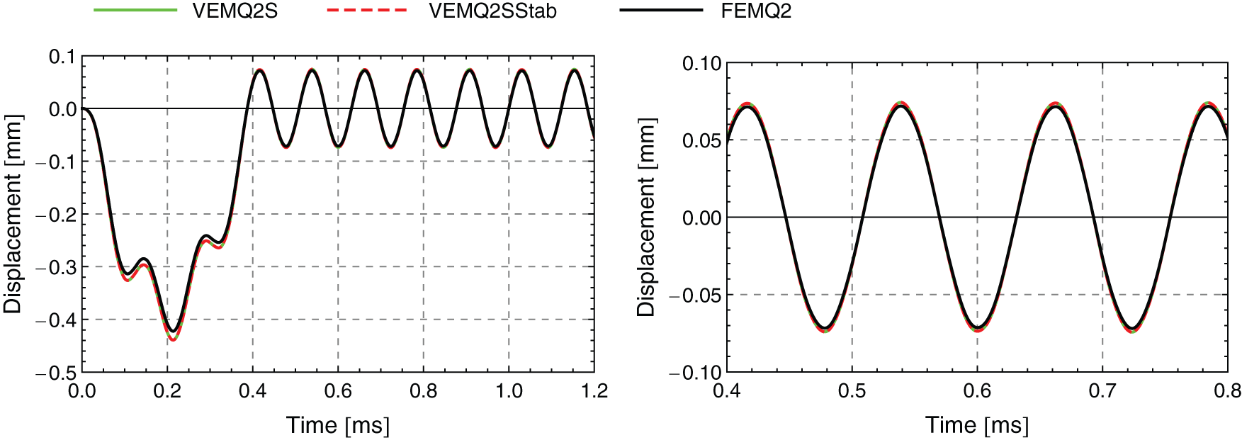
Figure 10: Displacement over time response at
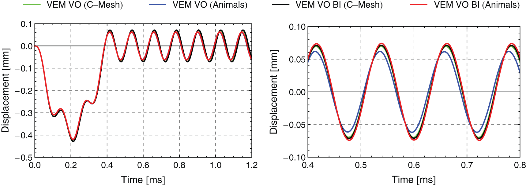
Figure 11: Displacement over time response at
The comparison of the different meshes shows, that the C-mesh yields a higher deflection, compared to the other results. Nevertheless qualitatively the shape of the displacement over time response fits very well the finite element FEM Q2 results and the virtual element VEM Q2S results. Again, the evaluation of the integral at the centroid of the element compared to computing the integral at the boundary exactly using the moments of area does not affect the results.
The next example is the Cook’s membrane problem in 2D. Here as well the virtual element performance will be compared with the finite element results. The geometrical setup and boundary conditions are demonstrated in Fig. 12b. In this test a force driven scenario is applied at the right edge as a line load as depicted in Fig. 12b. The force is applied as shown in Fig. 8b with
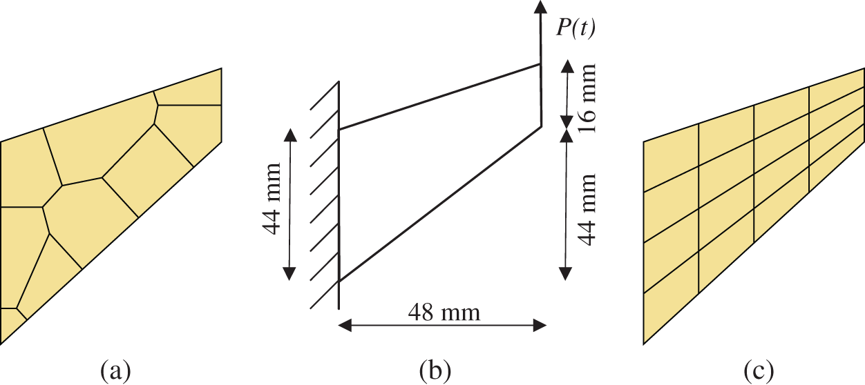
Figure 12: 2D example–-Cook’s membrane. VEM Voronoi Mesh (a), boundary value problem (b) and VEM Q2S Mesh (c)
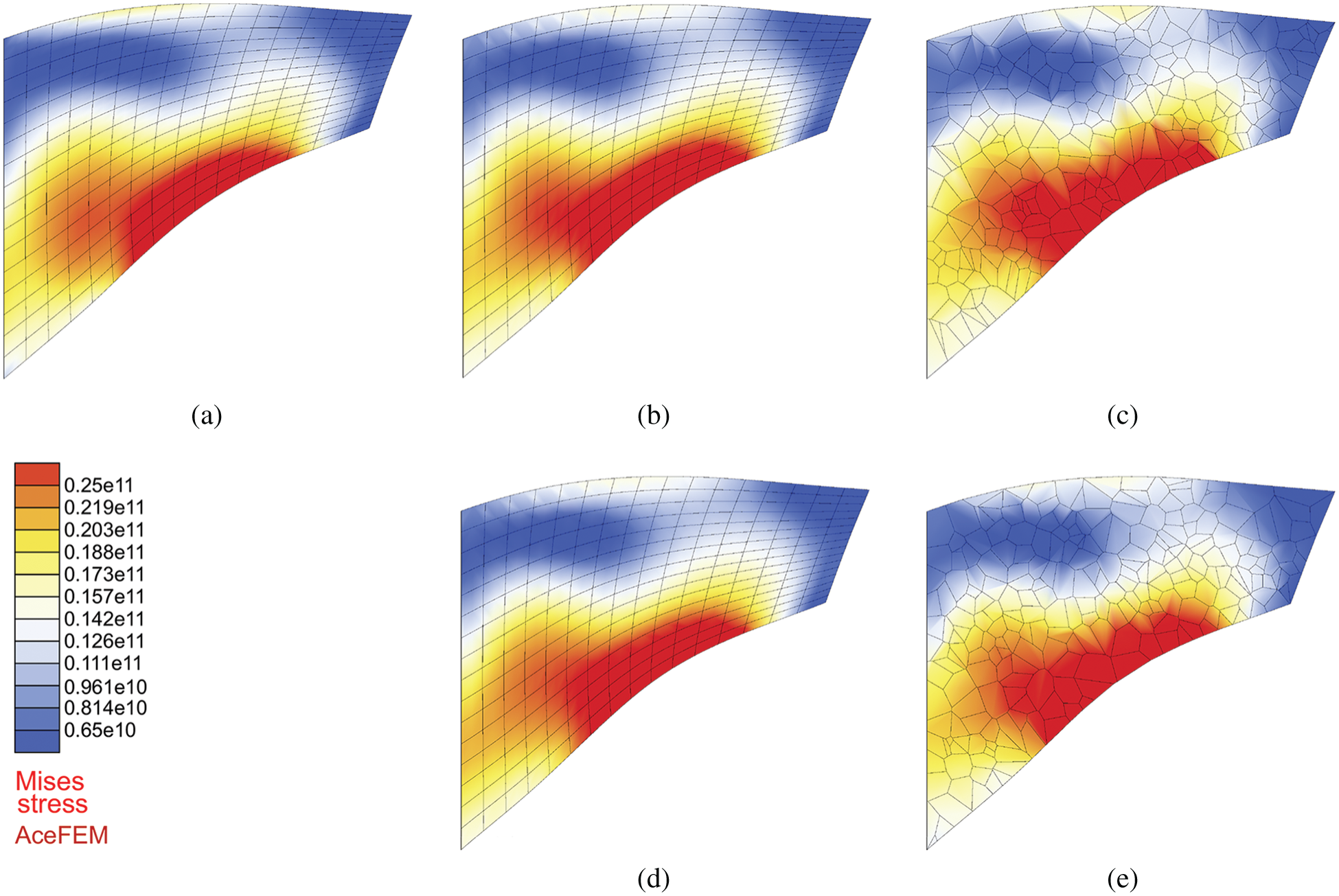
Figure 13: 2D example–-Cook’s membrane. Von Mises stress distribution at time
Fig. 14 shows a mesh refinement study with the element division of
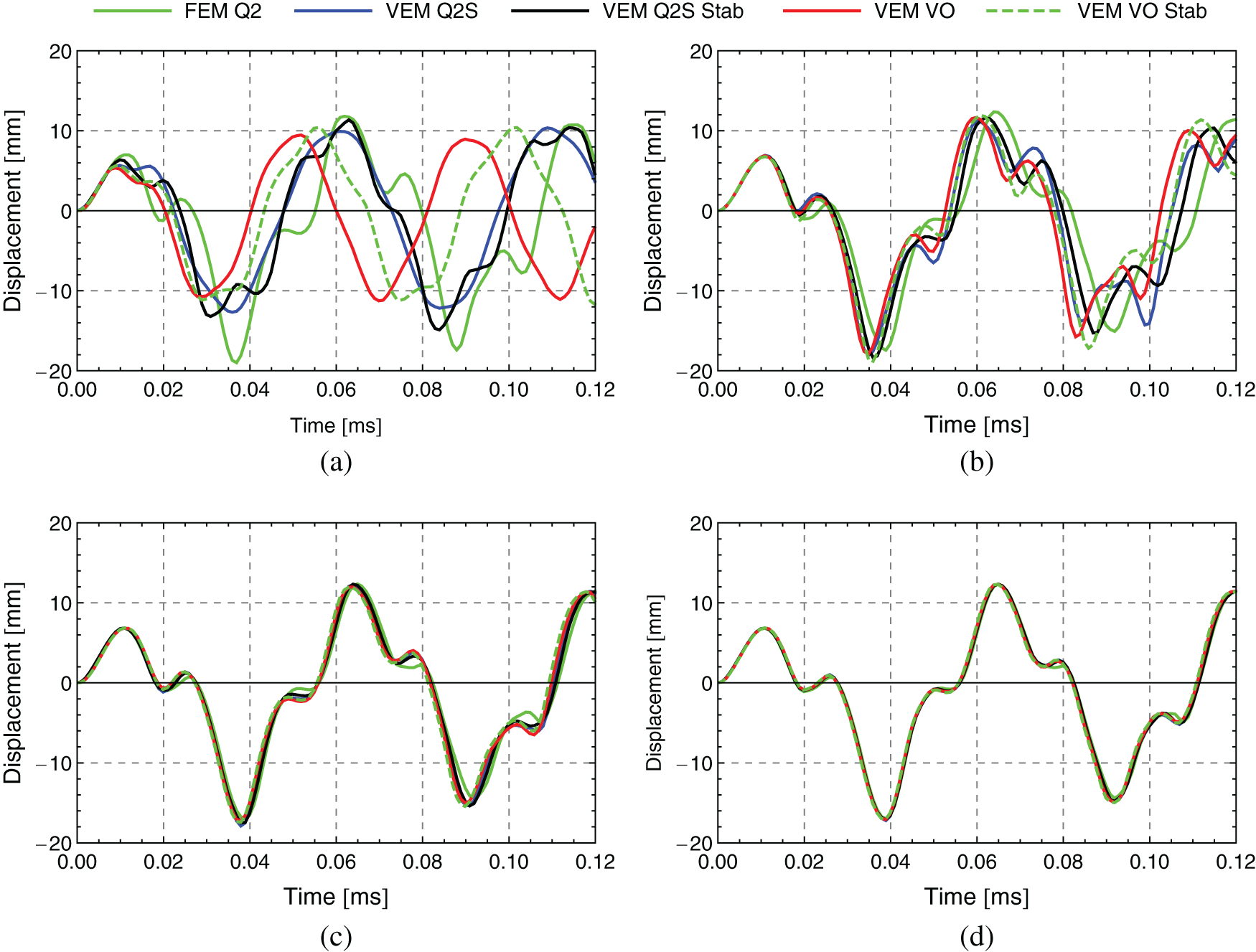
Figure 14: Convergence study–-Displacement over time response for 2D example–-Cook’s membrane. Element division
This study shows that again, that the evaluation of the integral of the dynamic part in (30) at the element centroid is absolutely sufficient to compute the mass matrix and that an element with a rank deficient mass matrix reproduces almost identical responses.
5.3 3D Boundary Value Problems
5.3.1 Wave Propagation in a Bar
The previously introduced 2D model of a bar is here extended to the third dimension. The length of the bar is set to
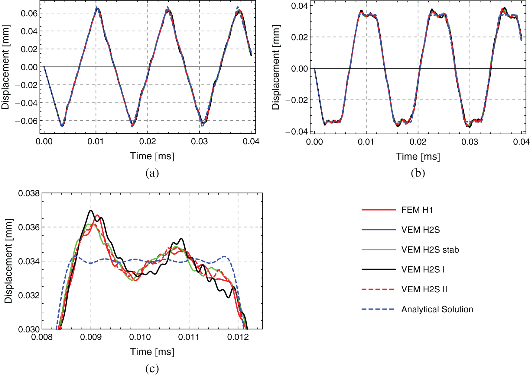
Figure 15: Displacement over time response for 3D example-Wave propagation in a bar that having an initial velocity of
5.3.2 Transversal Vibration of a Thick Beam
In this benchmark test a 3D cantilever beam is investigated. The geometric setup and the loading conditions of the specimen are depicted in Fig. 16. Here a line load is applied along the upper edge at the end of the beam with
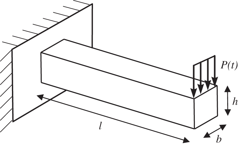
Figure 16: 3D example–-Transversal vibration of a thick beam (boundary value problem)
Additionaly, we employ the virtual element VEM H2S computed with 256 elements in Fig. 17a and compare it with the reference solution (FEM H2 with 3200 elements). It is interesting to note that despite the use of linear ansatz functions VEM H2S produces nearly the same results as the reference solution. This is due to the fact that the stabilization uses the bending modes. In conclusion, the presented formulation depicts very good results also in the 3D case.
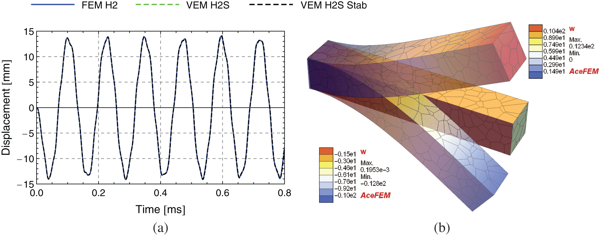
Figure 17: 3D example–-Transversal vibration of a thick beam. (a) Displacement over time response at
This test also confirms that evaluating the integral of the dynamic part in (30) for the computation of the mass matrix only at the centroid of the polygon/polyhedra is absolutely enough to get satisfying results. Furthermore, the virtual elements with stabilized and non-stabilized mass matrix lead to similar results. This again shows, that a rank deficient mass matrix can also be employed to use this virtual elements for elastodynamic problems. However, for higher frequencies, further investigations need to be done.
Since the resulting stresses play an important role in engineering applications, Fig. 18 shows the von Mises stress distribution at time
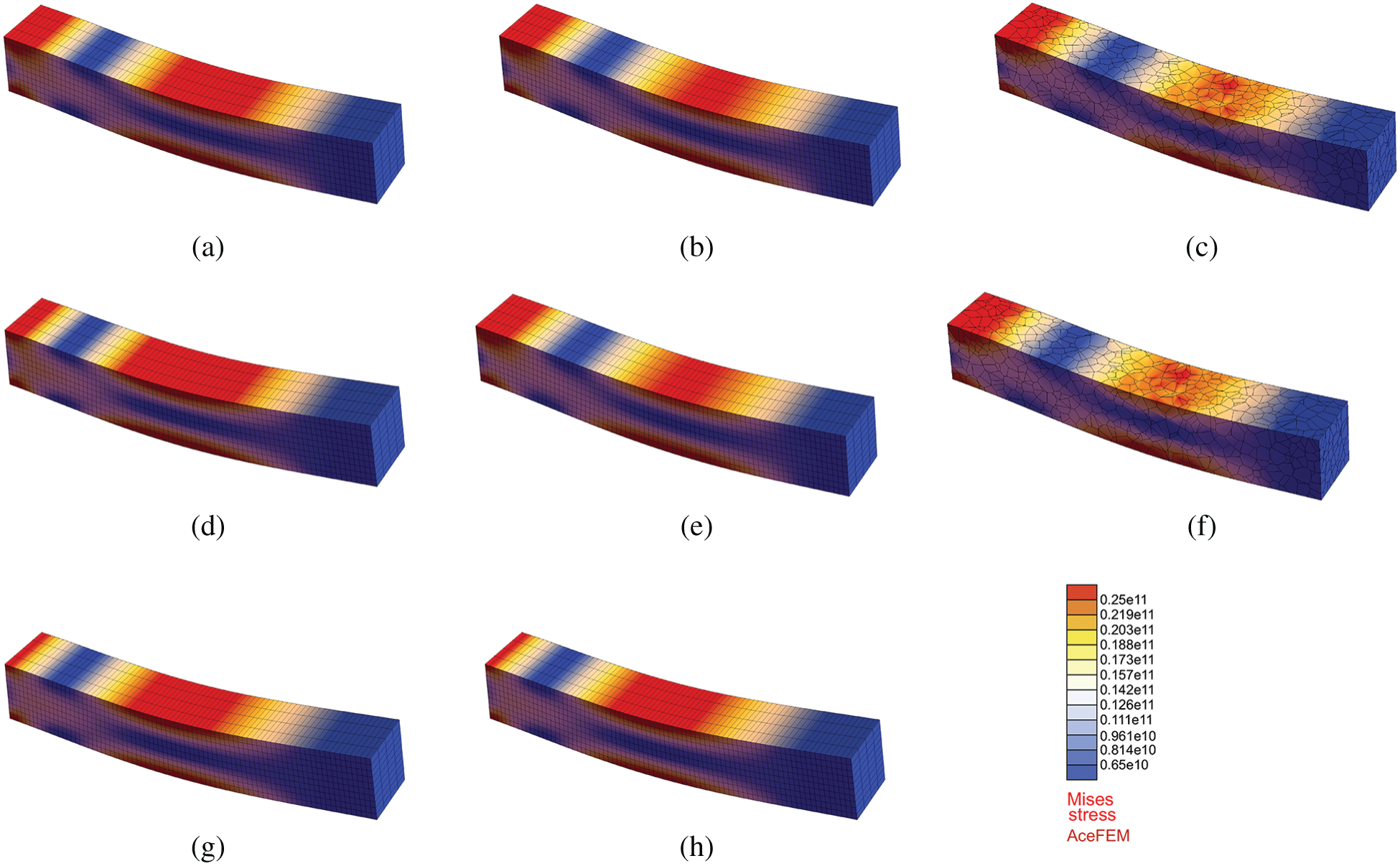
Figure 18: 3D example–-Transversal vibration of a thick beam. Von Mises stress distribution at time t = 0.1 ms for different elements. (a) FEM H1 (b) VEM H1 (c) VEM VO (d) FEM H2 (e) VEM H1 Stab (f) VEM VO Stab (g) VEM H2S (h) VEM H2S Stab
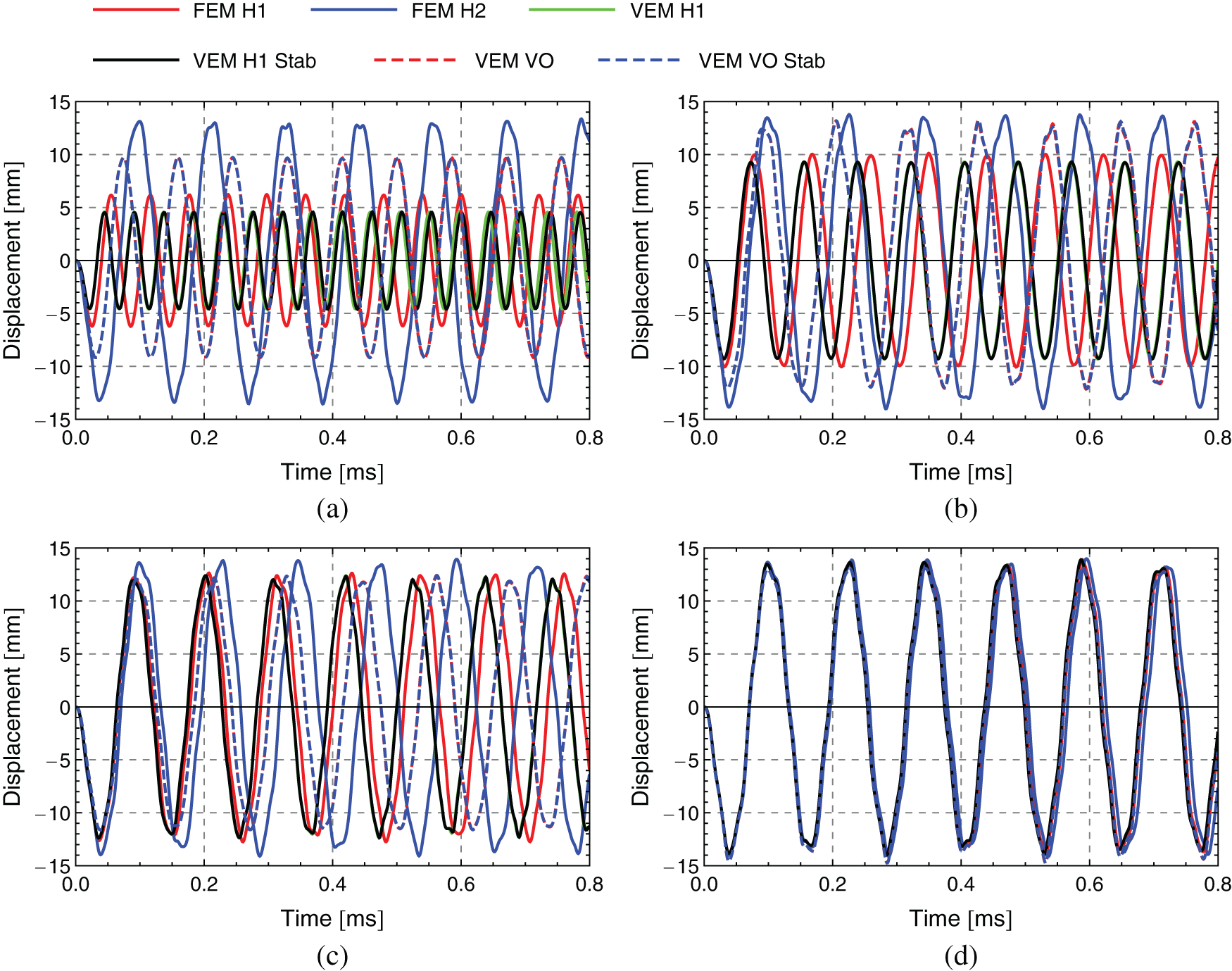
Figure 19: Convergence study–-Displacement over time response for 3D example–-Transversal vibration of a thick beam. Element division 2N, where N increases from (a) to (d). (a) N = 1 (b) N = 2 (c) N = 3 (d) N = 4
5.3.3 Vibration of a Thick Plate
The last example is related to the vibration of a thick plate which is discretized using three-dimensional elements. The plate has a length
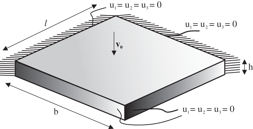
Figure 20: 3D example–-Vibration of a thick plate (boundary value problem)
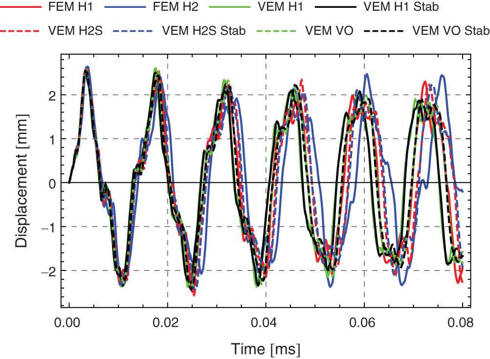
Figure 21: 3D example–-Vibration of a thick plate. Vertical displacement over time response at the center of the plate
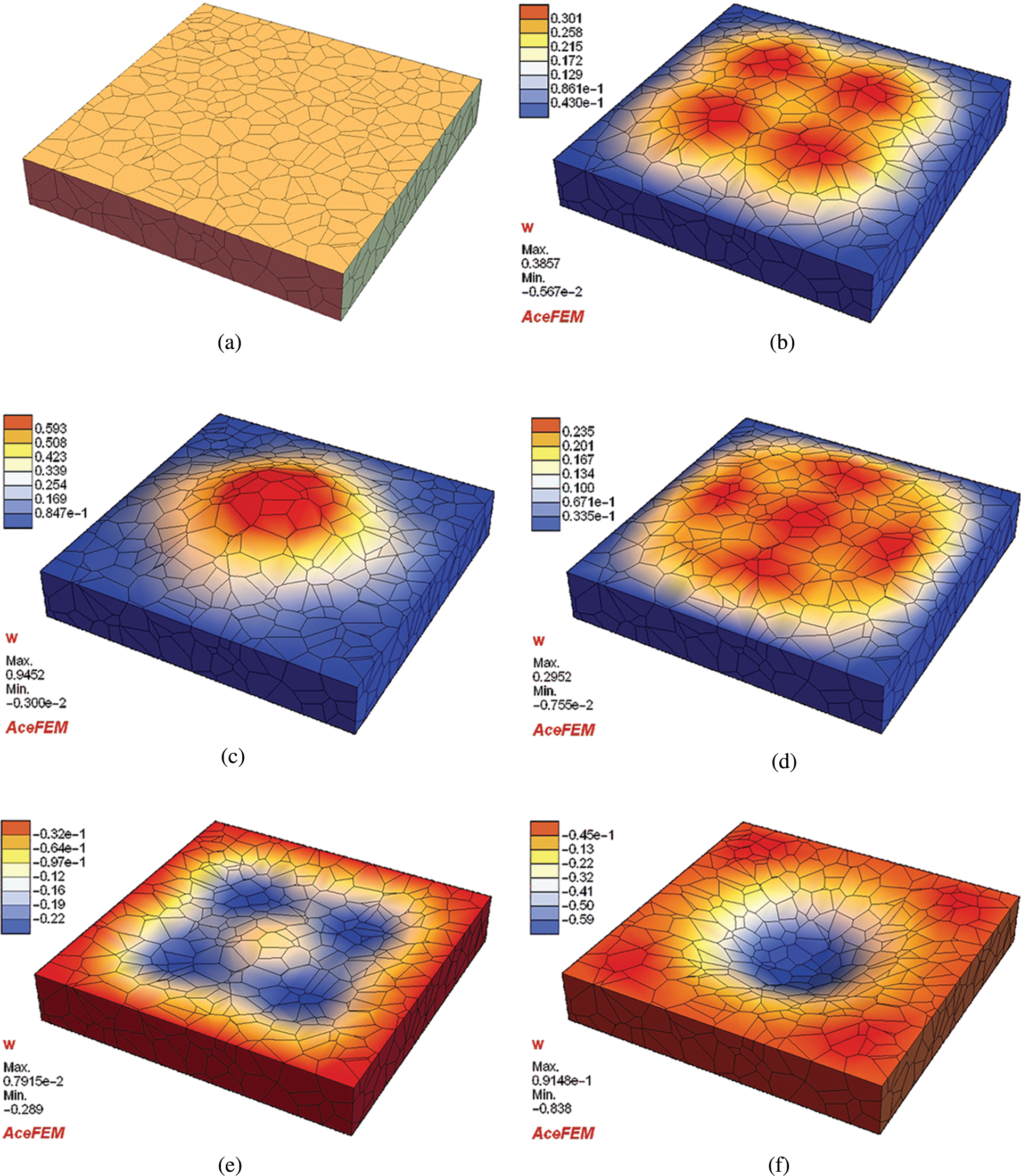
Figure 22: 3D example–-Vibration of a thick plate. Evolution of the displacement in the z-direction for different deformation states. (a) t = 0 s (b) t = 0.0000014798 (c) t = 0.00000290479 (d) t = 0.00000535609 (e) t = 0.000007597 (f) t = 0.00000989465
In this work, an efficient low order virtual element formulation for nonlinear elastodynamic was developed. The presented contribution does not consider the effect of damping, which can be included in further works. A formulation that derives single tangent matrix of dynamics problem is derived. The Newmark time discretization is performed within element itself. Thus the only unknowns of our problem are nodal displacements whereas the mass matrix is not required for solving simulations. However, the mass matrix can simply be exported, for eigenvalue analysis if required. Further solving the elastodynamics problem, employing the Newmark time integration on a global level will lead to similar results. Various schemes to integrate the dynamic part were shown, with and without stabilization. It was shown that the dynamic part does not need to be stabilized for the correctness and convergence of the procedure, unless eigenvalue analysis is needed. The virtual element results show a very good match with finite elements and analytical results for boundary and initial value problems. Arbitrary shaped elements with a various number of nodes could be used successfully for the simulations.
It shows that within this framework, the stabilization of the mass matrix is not needed. This is valid only for problems, where the equations are not reaction dominated [28,31]. To compute the integral of the dynamic part in Eq. (30), the argument can be evaluated at the element centroid. This is sufficiently accurate as shown in the examples. Hence, there is no need to perform any sub-triangulation of the element or use the moment of areas in (35) for the computation of the mass matrix.
The extension of VEM to other applications open a wide range of new research directions such as dynamic elasto-plasticity, contact or impact. Further we want to emphasize, that further investigations to high frequency applications, such as impact problems would also be interesting.
1Starting from a potential form is advantageous when using automatic differentiation, like the software tool AceGen. In this way the most efficient code for the residuals and consistent tangent operators of the virtual element will be generated for elastodynamic problems, see [26].
Funding Statement: The authors gratefully acknowledges support for this research by the “German Research Foundation” (DFG) in (i) the Collaborative Research Center CRC 1153 and (ii) the Priority Program SPP 2020.
Conflicts of Interest: The authors declare that they have no conflicts of interest to report regarding the present study.
1. Beiro da Veiga, L., Brezzi, F., Cangiani, A., Manzini, G., Marini, L. D. et al. (2013). Basic principles of virtual element methods. Mathematical Models and Methods in Applied Sciences, 23(1), 199–214. DOI 10.1142/S0218202512500492. [Google Scholar] [CrossRef]
2. Beião da Veiga, L., Brezzi, F., Marini, L. D. (2013). Virtual elements for linear elasticity problems. SIAM Journal on Numerical Analysis, 51(2), 794–812. DOI 10.1137/120874746. [Google Scholar] [CrossRef]
3. Gain, A. L., Talischi, C., Paulino, G. H. (2014). On the virtual element method for three-dimensional linear elasticity problems on arbitrary polyhedral meshes. Computer Methods in Applied Mechanics and Engineering, 282(2), 132–160. DOI 10.1016/j.cma.2014.05.005. [Google Scholar] [CrossRef]
4. Artioli, E., Beião da Veiga, L., Lovadina, C., Sacco, E. (2017). Arbitrary order 2D virtual elements for polygonal meshes: Part I, elastic problem. Computational Mechanics, 60(3), 355–377. DOI 10.1007/s00466-017-1404-5. [Google Scholar] [CrossRef]
5. Wriggers, P., Rust, W. T., Reddy, B. D. (2016). A virtual element method for contact. Computational Mechanics, 58(6), 1039–1050. DOI 10.1007/s00466-016-1331-x. [Google Scholar] [CrossRef]
6. Hudobivnik, B., Aldakheel, F., Wriggers, P. (2018). Low order 3D virtual element formulation for finite elasto-plastic deformations. Computational Mechanics, 63(2), 253–269. DOI 10.1007/s00466-018-1593-6. [Google Scholar] [CrossRef]
7. Aldakheel, F., Hudobivnik, B., Wriggers., P. (2019). Virtual elements for finite thermo-plasticity problems. Computational Mechanics, 64(5), 1347–1360. DOI 10.1007/s00466-019-01714-2. [Google Scholar] [CrossRef]
8. Artioli, E., Beião da Veiga, L., Lovadina, C., Sacco, E. (2017). Arbitrary order 2D virtual elements for polygonal meshes: Part II, inelastic problem. Computational Mechanics, 60(4), 643–657. DOI 10.1007/s00466-017-1429-9. [Google Scholar] [CrossRef]
9. Wriggers, P., Hudobivnik, B., Korelc, J. (2017). Efficient low order virtual elements for anisotropic materials at finite strains. Advances in computational plasticity, pp. 417–434. Berlin, Germany: Springer. [Google Scholar]
10. Wriggers, P., Hudobivnik, B., Schröder, J. (2018). Finite and virtual element formulations for large strain anisotropic material with inextensive fibers. Multiscale modeling of heterogeneous structures, pp. 205–231. Berlin, Germany: Springer. [Google Scholar]
11. Reddy, B. D., van Huyssteen, D. (2019). A virtual element method for transversely isotropic elasticity. Computational Mechanics, 64(4), 971–988. DOI 10.1007/s00466-019-01690-7. [Google Scholar] [CrossRef]
12. Artioli, E., Beião da Veiga, L., Dassi, F. (2020). Curvilinear virtual elements for 2D solid mechanics applications. Computer Methods in Applied Mechanics and Engineering, 359(1), 112667. DOI 10.1016/j.cma.2019.112667. [Google Scholar] [CrossRef]
13. Chi, H., Beião da Veiga, L., Paulino, G. (2017). Some basic formulations of the virtual element method (VEM) for finite deformations. Computer Methods in Applied Mechanics and Engineering, 318(1), 148–192. DOI 10.1016/j.cma.2016.12.020. [Google Scholar] [CrossRef]
14. Wriggers, P., Reddy, B., Rust, W., Hudobivnik, B. (2017). Efficient virtual element formulations for compressible and incompressible finite deformations. Computational Mechanics, 60(2), 253–268. DOI 10.1007/s00466-017-1405-4. [Google Scholar] [CrossRef]
15. Hussein, A., Aldakheel, F., Hudobivnik, B., Wriggers, P., Guidault, P. A. et al. (2019). A computational framework for brittle crack-propagation based on efficient virtual element method. Finite Elements in Analysis and Design, 159(1), 15–32. DOI 10.1016/j.finel.2019.03.001. [Google Scholar] [CrossRef]
16. Aldakheel, F., Hudobivnik, B., Hussein, A., Wriggers, P. (2018). Phase-field modeling of brittle fracture using an efficient virtual element scheme. Computer Methods in Applied Mechanics and Engineering, 341(39), 443–466. DOI 10.1016/j.cma.2018.07.008. [Google Scholar] [CrossRef]
17. Hussein, A., Hudobivnik, B., Wriggers, P. (2020). A combined adaptive phase field and discrete cutting method for the prediction of crack paths. Computer Methods in Applied Mechanics and Engineering, 372(2), 113329. DOI 10.1016/j.cma.2020.113329. [Google Scholar] [CrossRef]
18. Park, K., Chi, H., Paulino, G. (2019). On nonconvex meshes for elastodynamics using virtual element methods with explicit time integration. Computer Methods in Applied Mechanics and Engineering, 356(1), 669–684. DOI 10.1016/j.cma.2019.06.031. [Google Scholar] [CrossRef]
19. Beião da Veiga, L., Lovadina, C., Mora, D. (2015). A virtual element method for elastic and inelastic problems on polytope meshes. Computer Methods in Applied Mechanics and Engineering, 295(2), 327–346. DOI 10.1016/j.cma.2015.07.013. [Google Scholar] [CrossRef]
20. Nadler, B., Rubin, M. (2003). A new 3-D finite element for nonlinear elasticity using the theory of a cosserat point. International Journal of Solids and Structures, 40(17), 4585–4614. DOI 10.1016/S0020-7683(03)00210-5. [Google Scholar] [CrossRef]
21. Boerner, E. F. I., Loehnert, S., Wriggers, P. (2007). A new finite element based on the theory of a cosserat point-extension to initially distorted elements for 2D plane strain. International Journal for Numerical Methods in Engineering, 71(4), 454–472. DOI 10.1002/nme.1954. [Google Scholar] [CrossRef]
22. Krysl, P. (2016). Mean-strain 8-node hexahedron with optimized energy-sampling stabilization. Finite Elements in Analysis and Design, 108(3), 41–53. DOI 10.1016/j.finel.2015.09.008. [Google Scholar] [CrossRef]
23. Newmark, N. M. (1959). A method of computation for structural dynamics. Proceedings of ASCE, Journal of Engineering Mechanics, 85, 67–94. DOI 10.1061/JMCEA3.0000098. [Google Scholar] [CrossRef]
24. Wood, W. L. (1990). Practical time-stepping schemes. Oxford: Clarendon Press. [Google Scholar]
25. Wriggers, P. (2008). Nonlinear finite element methods. Berlin, Heidelberg: Springer. [Google Scholar]
26. Korelc, J., Wriggers, P. (2016). Automation of finite element methods. Berlin: Springer. [Google Scholar]
27. Korelc, J., Stupkiewicz, S. (2014). Closed-form matrix exponential and its application in finite-strain plasticity. International Journal for Numerical Methods in Engineering, 98(13), 960–987. DOI 10.1002/nme.4653. [Google Scholar] [CrossRef]
28. Beião da Veiga, L., Brezzi, F., Marini, L. D., Russo, A. (2014). The Hitchhiker’s guide to the virtual element method. Mathematical Models and Methods in Applied Sciences, 24(8), 1541–1573. DOI 10.1142/S021820251440003X. [Google Scholar] [CrossRef]
29. Singer, M. H. (1993). A general approach to moment calculation for polygons and line segments. Pattern Recognition, 26(7), 1019–1028. DOI 10.1016/0031-3203(93)90003-F. [Google Scholar] [CrossRef]
30. Petersen, C. (2013). Stahlbau-Grundlagen der Berechnung und Bauliche Ausbildung von Stahlbauten, vol. 4. Berlin, Germany: Springer. [Google Scholar]
31. Ahmad, B., Alsaedi, A., Brezzi, F., Marini, L., Russo, A. (2013). Equivalent projectors for virtual element methods. Computers & Mathematics with Applications, 66(3), 376–391. DOI 10.1016/j.camwa.2013.05.015. [Google Scholar] [CrossRef]
 | This work is licensed under a Creative Commons Attribution 4.0 International License, which permits unrestricted use, distribution, and reproduction in any medium, provided the original work is properly cited. |