| Computer Modeling in Engineering & Sciences |
DOI: 10.32604/cmes.2021.017404
ARTICLE
A Hybrid Immersed Boundary/Coarse-Graining Method for Modeling Inextensible Semi-Flexible Filaments in Thermally Fluctuating Fluids
Dedicated to Professor Karl Stark Pister for his 95th birthday
Department of Mechanical Engineering, University of California, Berkeley, CA, 94720-1740, USA
*Corresponding Author: Panayiotis Papadopoulos. Email: panos@berkeley.edu
Received: 08 May 2021; Accepted: 16 July 2021
Abstract: A new and computationally efficient version of the immersed boundary method, which is combined with the coarse-graining method, is introduced for modeling inextensible filaments immersed in low-Reynolds number flows. This is used to represent actin biopolymers, which are constituent elements of the cytoskeleton, a complex network-like structure that plays a fundamental role in shape morphology. An extension of the traditional immersed boundary method to include a stochastic stress tensor is also proposed in order to model the thermal fluctuations in the fluid at smaller scales. By way of validation, the response of a single, massless, inextensible semiflexible filament immersed in a thermally fluctuating fluid is obtained using the suggested numerical scheme and the resulting time-averaged contraction of the filament is compared to the theoretical value obtained from the worm-like chain model.
Keywords: Semiflexible biopolymers; immersed boundary method; coarse-graining; actin filaments; fluid-structure interaction; thermal fluctuations; persistence length
Living cells display a high degree of internal mechanical and functional organization and their intracellular biopolymeric scaffold, the cytoskeleton, plays a key role in that [1]. The actin cortex is the part of the cytoskeleton attached to the cell membrane in most eukaryotic cells. The cortical actin cytoskeleton plays a fundamental role in cell shape, which is maintained through structural stiffness and rheology. Actin cortex is a thin actomyosin network that underlies the plasma membrane, consisting of actin filaments cross-linked by actin-binding proteins and containing motor proteins that generate stress within the network [2]. In order for the actin filaments to become cross-linked, they undergo thermal fluctuations to find a cross-linking partner and when cross-links between actin filaments are formed, the amplitudes of filament fluctuations are reduced, supporting the formation of additional cross-links [3].
Actin filaments are biopolymers with sufficient contour length to exhibit significant thermal bending fluctuations, in the order of approximately 1% of their contour length. However, their diameter can be as large as ten nanometers or more, giving them noteworthy bending rigidity. Thus, actin filaments are said to be semiflexible in the sense that their bending stiffness is large enough for the bending energetics—which favors a straight conformation—to just out-compete the entropic tendency of a chain to crumple up into a random coil [4]. Therefore, semiflexible polymers exhibit small, yet significant, thermal fluctuations around a straight conformation. Furthermore, the semiflexible filaments are practically inextensible, i.e., their backbone cannot be stretched or compressed. On the scale of several nanometers to micrometers, biopolymers are often effectively modeled as inextensible elastic rods or fibers with finite resistance to bending [5]. This is the essence of the classical worm-like chain (WLC) model by Kratky et al. [6]. The competition between entropic and energetic effects in semiflexible polymers gives rise to many physical properties and the semiflexible nature of the actin filaments also has major implications on how they interact with each other to form cross-linked networks [7,8]. One may think of a single actin filament as a chain that can respond to forces or thermal fluctuations by bending and end-to-end compression relative to its full contour length.
There has been deep interest in studying the mechanical response of biological tissues the past decades, and more specifically, in understanding the mechanical properties of biopolymeric networks, since they play an important role in cell motility [9,10] and mechanotransduction [11–13]. Furthermore, the investigation of the behavior of semiflexible filaments in viscous shear flows at low Reynolds numbers has also gained a lot of interest due to the relevance of its applications in areas involving biological systems like DNA [14,15], polymers [16] and proteins, but also in areas such as biotechnology that involve natural and synthetic fibers [17]. These fluid-structure interaction (FSI) problems are quite challenging because of the complex interplay of hydrodynamic stresses and the corresponding fiber conformity, however, a two-way interaction between the immersed filaments and the surrounding fluid is tantamount in order to get a better understanding of the underlying physical behavior.
Yamamoto et al. [18] proposed a method for simulating the dynamic behavior of rigid and flexible fibers in a flow field, with the fibers regarded as made up of spheres that are lined up and bonded to each neighbor. Tornberg et al. [19] studied the dynamics of slender filaments suspended in Stokesian fluids employing a non-local slender body theory. In most of these studies, the hydrodynamic interaction was neglected, therefore, there was limited information about the underlying FSI. The fluid was considered as a passive medium and coupling between fluid and structure was one-way. The Immersed Boundary Method (IBM) of Peskin [20], which accounts for the two-way interaction between filament and fluid, has gained substantial popularity the past years in studying the dynamics of filaments in flow fields. However, in most of the studies where the dynamics of inextensible semiflexible filaments were studied using IBM, as in [21,22], a very high stretching stiffness was used for the filaments to approximate inextensibility, which significantly restricted the time step, thus increasing substantially the computational cost. Wiens et al. [23] used a generalized IB method which can be viewed as a type of penalty method in which the rod is only approximately inextensible. Similarly, Huang et al. [24] used a modified IBM with an extra inextensibility condition to strictly enforce the filament inextensibility. In addition, Kim et al. [25] introduced a penalty immersed boundary method to simulate the dynamics of inextensible vesicles in an incompressible viscous fluid by using two Lagrangian immersed boundaries connected through stiff springs to represent the real immersed boundary for different purposes. Also, Ong et al. [26] developed an immersed boundary projection method based on an unconditionally energy stable scheme to simulate the vesicle dynamics in a viscous fluid.
In the preceding studies the inextensibility constraint is not enforced strongly and this may lead to numerical errors [24] that cause the filament length to vary over time. On the other hand, when inextensibility is enforced by Lagrange multipliers, an extended nonlinear system of equations needs to be solved at every time step, thus again increasing substantially the computational time. An alternative primal approach, more straightforward and faster computationally, to deal with the inextensibility of semiflexible filaments is to use the Coarse-Graining Method (CGM) by Moreau et al. [27]. CGM uses discrete models, where the filament is partitioned into a discrete number of straight segments and the elastic interaction coupling neighboring nodes/joints is described via discrete elastic connectors encoding the filament's resistance to bending. However, up to now, the CGM for filaments has been used by neglecting the two-way interaction between the filament and the fluid.
In this study, a new computationally efficient version of the IBM, which is combined with the CGM, is introduced in this study for modeling inextensible filaments in low-Reynolds number flows. An extension of the traditional IBM to include a stochastic stress tensor is also proposed in order to model the thermal fluctuations in the fluid in smaller scales. The proposed numerical scheme is validated by comparing the response of a single actin filament immersed in a thermally fluctuating fluid to the theoretical values obtained using the WLC model.
The remainder of the article is organized as follows. The WLC model is reviewed in Section 2 and the theoretical value of the time-averaged contraction for a single inextensible filament under hydrodynamic thermal fluctuations is derived. The mathematical formulation of the coupled system filament-fluid and the suggested numerical procedure are described in Section 3. In Section 4, the behavior of a single, massless, inextensible, and semiflexible filament immersed in a thermally fluctuating fluid is obtained using the suggested numerical scheme and the resulting time-averaged contraction of the filament is compared to the theoretical value obtained from the WLC model for the sake of validation. This is followed by a concluding reflection on the findings in Section 5.
2 Theoretical Background: The Worm-Like Chain Model
The mechanical behavior of semiflexible filaments is usually described by the WLC model [6]. This assumes that the filament is inextensible, has linearly elastic bending energy, and is subjected to thermal fluctuations. A homogeneous, inextensible and semiflexible filament of straight length L and circular cross section of radius a is taken to be fixed at one end and free at the other. The domain of the filament is parametrized by its arc-length s and the position of a typical point is denoted y(s). The motion of the filament is assumed to be confined to a plane and its bending energy is given by
where
Using the Equipartition Theorem [28, Chapter 7] one may calculate the thermal average angular correlation between distant points along the filament, for which
where
For the filament under consideration here, it is assumed that L≤ lp, therefore it is expected to remain nearly straight with small transverse fluctuations. Let the x-axis define the average orientation of the filament segment, and let u represent the transverse displacement taken to be a function of x and time t. The function u(x, t) may be represented by a Fourier series as
where q are the wave numbers defined as q = nπ/L, where n = 1, 2, 3,…, and uq are the corresponding amplitudes. Such a representation is appropriate for the case of a nearly straight filament with boundary condition u = 0 at x = 0 and no restraint at x = L, as in Fig. 1. Since the transverse displacement is assumed infinitesimal, the local orientation and curvature of the filament are given by
as also in [29].
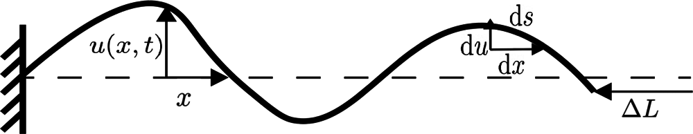
Figure 1: Configuration of filament fixed at one end, where u(x; t) denotes the transverse displacement u from an initial straight line (dashed). The magnitude of u is exaggerated for illustration
Since the filament is inextensible, the total arc-length of the filament remains unchanged under the influence of the fluctuations. Thus, the arc length ds of a short segment is approximately given by
where use is made of the approximation
By way of background, recall that the ensemble average <A(t)> of an observable quantity A, which is a function of a variable
see, e.g., [30, Chapter 3]. Here, γ is the phase space of
In the context of the present problem, if the filament is in equilibrium at temperature T, the ensemble average value
where
where “ln” denotes the natural logarithm. A straightforward calculation results in
therefore, for any q, the ensemble average of the amplitude-squared is written as
in terms of the original length L and the persistence length lp. Likewise, using (6) and (11), the ensemble average <ΔL> of the contraction ΔL is expressed as
It can be observed from (11) that the ensemble average of the amplitude-squared of the bending fluctuations diminishes rapidly for higher-order modes due to the (negative) fourth-power dependence on the wave number. Also, (12) implies that the longer the persistence length, the smaller the ensemble average of the contraction Δ L.
The probability density function f in (7) is independent rendering the ensemble stationary. In this case, the ergodic hypothesis [28, Chapter 15] states then that the ensemble average over all accessible systems is equal to the time average over a large number of observation of a single system. That is, given any observable quantity A in a stationary ensemble,
for sufficiently large observation time t. Therefore, the ensemble averages
3 Mathematical Formulation and Numerical Procedure
The fluid and the immersed semiflexible filament constitute a coupled mechanical system. The inextensible filament's motion is driven by the fluid's velocity field, while, at the same time, the filament exerts force on the fluid, thus affecting its motion. The equations of motion that describe the coupled system are derived and discussed in the remainder of this section.
3.1 The Asymptotic Coarse-Grained Elastohydrodynamics
Consider an inextensible massless filament of length L immersed in an incompressible viscous fluid, and recall that the position of a point of the rod be denoted by y(s). The filament is embedded in a two-dimensional space associated with orthonormal basis {ex, ey} and is subjected to external contact force fh(s) per unit length due to the hydrodynamic interactions.
Assuming quasi-static loading conditions, the equilibrium equations are written as
where n and m are the (internal) axial force and moment sustained by the filament. Integrating the force equilibrium Eq. (14)1 over the entire filament leads to
where it is further assumed that the boundary forces vanish, that is, n(0) = n(L) = 0.
Following Moreau et al. [27], the filament is partitioned into N straight subdomains (elements) of length Δs = L/N. The Frenet basis along the filament is given by the unit tangent and normal vectors (
where Fhi represents the resultant external force experienced by the i-th element. For a filament free of boundary moments, that is, assuming, m(L) = m(0) = 0, one may take the integral of (14)2 over the entire filament, use integration by parts, and invoke (14)1 and (16) to conclude that
where Mi,y0 is the moment of the external force acting on the i-th element about point y0 = y(0). Upon integrating Eq. (14)2 over the domain ((j − 1)Δs, L), j = 2,…,N, and taking into account (17), it follows that
where mj = m((j − 1)L/N), j = 2,…, N, is the moment at the left end-point of the j-th element. Given that the moment at any point it is defined as
where αj = θj − θj − 1, j = 1, 2,…,N, is the angle between ei − 1,∥ and ei ,∥, as shown in Fig. 2, and thus
with α0 = θ0 .
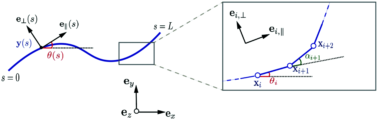
Figure 2: Parametrization of the continuous and discretized filament
In the low-Reynolds number regime, the hydrodynamic force experienced by the filament immersed in fluid with velocity field v can be defined according to the Resistive Force Theory [31] as
where v(y) is the fluid velocity interpolated at the filament positions, and ξ and η are the normal and tangential drag coefficients, respectively. Here, the external contact force fh(s) is due to the resistance that the filament points experience as they move in the fluid.
The position y at time t is a point in the filament that satisfies
for i = 1,… , N, thus yi = y((i − 1)L/N) thus satisfying the inextensibility constraint from the outset. Here, ek,∥ denotes the tangent Frenet vector in the k-th element.
There are now N + 2 parameters describing the position of the filament, that is, (y0, α0, …, αN − 1). To determine them, there are two total force balance equations in (16), one torque balance in (17), and N − 1 equations for the internal moment balance in (18), thus rendering this elastohydrodynamic system closed.
With slight abuse of notation, let yi(s) denote the current position of a filament point on the i-th element, so that
The total hydrodynamic force on the i-th element is found from (21), with the aid of (16) and (23), to be
Note that, in general, v varies along the domain (iΔs, (i\, + 1)Δs). However, to within a small error, the velocity is assumed constant in each element. Using Eqs. (17) and (21), one finds that
Therefore, Eqs. (16)–(18), with the aid of (24) and (25), take the form
These coarse-grained elastohydrodynamics equations, in conjunction with Eqs. (20) and (22), can be cast a system of ordinary differential equations of the form
where
The matrix [A] has dimensions (N + 2) × 3N and its coefficients are given, for all i, j = 0,…, N − 1, by
If j < i, then ai + 2,j = ai + 2,N + j = ai + 2,2N + j = 0. Also, the column vector [B] of size N + 2 is given by
In addition, matrix [Q] is a 3N × (N + 2) transformation matrix defined as
where [Q1] and [Q2] are N × N matrices whose elements are given by the general formula
with
The system of equations in (27) is integrated in time using an implicit first-order method with constant time step Δt. Writing the system of equations at time tn + 1, one can obtain [Yn + 1] by solving implicitly the system of equations
in the typical time domain (tn, tn + 1].
3.2 Hydrodynamic Fluctuations and Equations of Motion
As one approaches smaller length scales, in the order of μm, thermal fluctuations play an essential role in the description of the fluid flow. Thermal fluctuations may be included in the continuum description of the fluid by means of additional stochastic fluxes. The resulting equations of motion for the fluctuating fluid turn out to be stochastic partial differential equations. Landau et al. [32, Chapter 9] proposed such equations, which include an additional stochastic stress tensor in the Navier-Stokes equations, the so-called Landau-Lifshitz Navier-Stokes (LLNS) equations.
To account for thermal fluctuations, the Cauchy stress tensor T for an incompressible viscous fluid can be modified as
where p is the pressure, μ is the dynamic viscosity of the fluid, D is the rate-of-deformation tensor, and
where δ(⋅) is the Dirac delta function,
The low-Reynolds number Navier-Stokes equations for an incompressible, Newtonian fluid with the additional stochastic stress tensor to account for the thermal fluctuations can be written, in the absence of body forces, as
where, again, v is the fluid's velocity field and also ρ is the density of the incompressible fluid. As it turns out, the flow in cytosol is of low Reynolds number, in the order of 10−9, in large part due to the cell's size, which is in the order of μm [1]. For such flows it is reasonable to adopt the unsteady Stokes approximation, where the convective rate of change
Consider now an incompressible viscous fluid occupying a two-dimensional domain Ω and undergoing thermal fluctuations. The IBM formulation in its strong form can be understood as an enrichment of the two-dimensional Navier-Stokes equations accounting also for the forces generated by the deformation of the immersed body, with the linear momentum balance equations in (35)2 for the fluid taking the form
where F is the force that the filament exerts to the fluid.
In the discrete case, the force term F included in the Navier-Stokes equations is defined to be equal and opposite to the equivalent hydrodynamic force Fhi experienced by the fiber moving with the fluid with velocity field according to the Resistive Force Theory [31] and Eqs. (21) and (24). Also, the perpendicular and parallel drag coefficients in Eq. (21) for a filament of cross-sectional radius r and length 2l are defined, following Lighthill's classical analysis [33], as
There exist many choices for representing the stochastic stress tensor
where
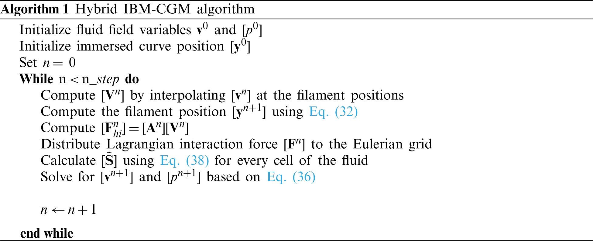
3.3 Summary of the Numerical Algorithm for the Hybrid IBM-CGM
The implementation of the proposed numerical algorithm for simulating flexible inextensible filaments immersed in a fluid can be summarized as follows:
This section focuses on the mechanical response of a single massless filament immersed in a thermally fluctuating fluid and aims to validate the results of the computational model described in the previous section by comparison with the theoretical prediction based on the WLC model in Section 2.
The biopolymers that comprise the cytoskeleton consist of aggregates of large globular proteins that are bound together rather weakly, as compared with most synthetic, covalently bonded polymers [5]. Nevertheless, they can be surprisingly strong, due to their relatively large diameter, which makes their bending rigidity the dominant attribute determining their mechanical behavior on the cellular scale. Even with this mechanical resistance to bending, however, cytoskeletal filaments can still exhibit significant thermally induced bending fluctuations because of Brownian motion in the surrounding fluid. Actin filaments, owing to their relatively large bending stiffness, have long persistence length compared to their total contour length, which practically means that an actin filament in thermal equilibrium in a fluid will appear rather straight. Here, the results of simulations of an inextensible filament immersed in a fluid domain with thermal noise are used to verify that, after a sufficient amount of time, the time-averaged contraction <ΔL>t of the filament approaches the theoretical value of the ensemble average <ΔL> derived in Section 2.
The inextensible filament is modeled by means of the CGM described in Section 3.1. The filament has contour length of
Fig. 3 depicts the results of the simulation described above. The time-averaged contraction <ΔL>t is plotted as a function of the number of time steps. It can be concluded from the plot that after around 6 ∗ 106 time steps, <ΔL>t converges to a value which is approximately equal to 3.31 × 10⁻¹³. This compares very well to the theoretical value for the ensemble average obtained from Eq. (12), which is approximately equal to 3.45 × 10⁻¹³ for a relative error of approximately 4%. In view of this agreement, the comparison may serve as validation of the proposed numerical algorithm used to simulate the fluid-structure interaction of the immersed filaments under thermal fluctuations.
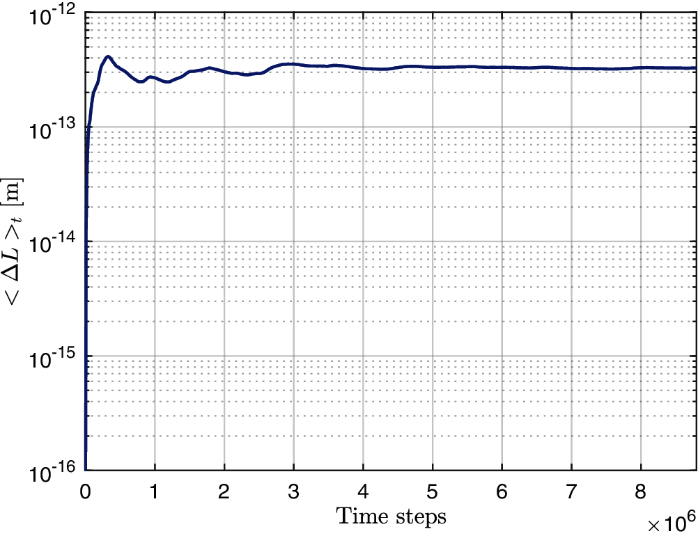
Figure 3: Time average (log scale) of inextensible filament's contraction <ΔL>t as a function of the number of time steps under thermal fluctuations
In this study, a modified and computationally efficient version of the Immersed Boundary Method, combined with the Coarse-Graining Method, was proposed for modeling inextensible semiflexible filaments in low-Reynolds number flows. Thermal fluctuations in the fluid were modeled by including a stochastic stress. The mechanical behavior of a massless, inextensible, and semiflexible filament immersed in a thermally fluctuating fluid was investigated using the suggested method. The resulting time-averaged contraction of the filament compares very favorably to the theoretical value for the ensemble average of the same quantity, as obtained from the Worm-like Chain model. On the basis of this analysis, the proposed hybrid algorithm appears to be both robust and accurate, and could offer a reliable means for investigating the combined effect of multiple (and possibly interacting) filaments in low-Reynolds number flows.
Funding Statement: The authors received no specific funding for this study.
Conflicts of Interest: The authors declare that they have no conflicts of interest to report regarding the present study.
1. Boal, D. H. (2012). Mechanics of the cell. Cambridge: Cambridge University Press. [Google Scholar]
2. Lodish, H., Kaiser, C., Krieger, M., Bretscher, A., Ploegh, H., et al., (2013). Molecular cell biology, 7th edition. New York: W. H. Freeman and Co. [Google Scholar]
3. Jensen, M. H., Morris, E. J., Goldman, R. D., Weitz, D. A. (2014). Emergent properties of composite semiflexible biopolymer networks. BioArchitecture, 4(5), 138–143. DOI 10.4161/19490992.2014.989035. [Google Scholar] [CrossRef]
4. Ambriz, X., de Lanerolle, P., Ambrosio, J. R. (2018). The mechanobiology of the actin cytoskeleton in stem cells during differentiation and interaction with biomaterials. Stem Cells International, 10(1), 42–47. DOI 10.1155/2018/2891957. [Google Scholar] [CrossRef]
5. Broedersz, C., MacKintosh, F. C. (2014). Modeling semiflexible polymer networks. Reviews of Modern Physics, 86(3), 995–1036. DOI 10.1103/RevModPhys.86.995. [Google Scholar] [CrossRef]
6. Kratky, O., Porod, G. (1949). Röntgenuntersuchung gelöster gadenmoleküle. Recueil des Travaux Chimiques des Pays-Bas, 68(12), 1106–1122. DOI 10.1002/recl.19490681203. [Google Scholar] [CrossRef]
7. Bausch, A. R., Kroy, K. (2016). A bottom-up approach to cell mechanics. Nature Physics, 2(4), 231–238. DOI 10.1038/nphys260. [Google Scholar] [CrossRef]
8. MacKintosh, F. C., Janmey, P. A. (1997). Actin gels. Current Opinion in Solid State and Materials Science, 2(3), 350–357. DOI 10.1016/S1359-0286(97)80127-1. [Google Scholar] [CrossRef]
9. Mitchison, T. J., Cramer, L. P. (1996). Actin-based cell motility and cell locomotion. Cell, 84(3), 371–379. DOI 10.1016/S0092-8674(00)81281-7. [Google Scholar] [CrossRef]
10. Carlier, M. F., Pantaloni, D. (1997). Control of actin dynamics in cell motility. Journal of Molecular Biology, 269(4), 459–467. DOI 10.1006/jmbi.1997.1062. [Google Scholar] [CrossRef]
11. Orr, A. W., Helmke, B. P., Blackman, B. R., Schwartz, M. A. (2006). Mechanisms of mechanotransduction. Developmental Cell, 10(1), 11–20. DOI 10.1016/j.devcel.2005.12.006. [Google Scholar] [CrossRef]
12. Schwartz, U. S., Gardel, M. L. (2012). United we stand-integrating the actin cytoskeleton and cell-matrix adhesions in cellular mechanotransduction. Journal of Cell Science, 125(13), 3051–3060. DOI 10.1242/jcs.093716. [Google Scholar] [CrossRef]
13. Harris, A. R., Jreij, P., Fletcher, D. A. (2018). Mechanotransduction by the actin cytoskeleton: Converting mechanical stimuli into biochemical signals. Annual Review of Biophysics, 47(1), 617–631. DOI 10.1146/annurev-biophys-070816-033547. [Google Scholar] [CrossRef]
14. Bustamante, C., Bryant, Z., Smith, S. (2003). Ten years of tension: Single-molecule DNA mechanics. Nature, 421(6921), 423–427. DOI 10.1038/nature01405. [Google Scholar] [CrossRef]
15. Peters, J. P., Yelgaonkar, S. P., Srivatsan, S. G., Tor, Y., Maher, J. L. (2013). Mechanical properties of DNA-like polymers. Nucleic Acids Research, 41(22), 10593–10604. DOI 10.1093/nar/gkt808. [Google Scholar] [CrossRef]
16. Kanchan, M., Maniyeri, R. (2019). Numerical analysis of the buckling and recuperation dynamics of flexible filament using an immersed boundary framework. International Journal of Heat and Fluid Flow, 77, 256–277. DOI 10.1016/j.ijheatfluidflow.2019.04.011. [Google Scholar] [CrossRef]
17. Gardel, M. L. (2013). Synthetic polymers with biological rigidity. Nature, 493(7434), 618–619. DOI 10.1038/nature11855. [Google Scholar] [CrossRef]
18. Yamamoto, S., Matsuoka, T. (1993). A method for dynamic simulation of rigid and flexible fibers in a flow field. The Journal of Chemical Physics, 98(1), 644–650. DOI 10.1063/1.464607. [Google Scholar] [CrossRef]
19. Tornberg, A. K., Shelley, M. J. (2004). Simulating the dynamics and interactions of flexible fibers in stokes flows. Journal of Computational Physics, 196(1), 8–40. DOI 10.1016/j.jcp.2003.10.017. [Google Scholar] [CrossRef]
20. Peskin, C. S. (2002). The immersed boundary method. Acta Numerica, 11, 479–517. DOI 10.1017/S0962492902000077. [Google Scholar] [CrossRef]
21. Stockie, J. M., Green, S. I. (1998). Simulating the motion of flexible pulp fibers using the immersed boundary method. Journal of Computational Physics, 147(1), 147–165. DOI 10.1006/jcph.1998.6086. [Google Scholar] [CrossRef]
22. Stockie, J. M. (2002). Simulating the dynamics of flexible wood pulp fibers in suspension. Proceedings of the 16th Annual International Symposium on High Performance Computing Systems and Applications, pp. 154–160, IEEE Computer Society, Atlanta. [Google Scholar]
23. Wiens, J. K., Stockie, J. M. (2015). Simulating flexible fiber suspensions using a scalable immersed boundary algorithm. Computer Methods in Applied Mechanics and Engineering, 290, 1–18. DOI 10.1016/j.cma.2015.02.026. [Google Scholar] [CrossRef]
24. Huang, W. X., Shin, S. J., Sung, H. J. (2007). Simulation of flexible filaments in a uniform flow by the immersed boundary method. The Journal of Chemical Physics, 226(2), 2206–2228. DOI 10.1016/j.jcp.2007.07.002. [Google Scholar] [CrossRef]
25. Kim, Y., Lai, M. C. (2010). Simulating the dynamics of inextensible vesicles by the penalty immersed boundary method. Journal of Computational Physics, Inc, 229(12), 4840–4853. DOI 10.1016/j.jcp.2010.03.020. [Google Scholar] [CrossRef]
26. Ong, K. C., Lai, M. C. (2020). An immersed boundary projection method for simulating the inextensible vesicle dynamics. Journal of Computational Physics, 408, 109277. DOI 10.1016/j.jcp.2020.109277. [Google Scholar] [CrossRef]
27. Moreau, C., Giraldi, L., Gadêlha, H. (2018). The asymptotic coarse-graining formulation of slender-rods, bio-filaments and flagella. Journal of the Royal Society Interface, 5(144), 20180235. DOI 10.1098/rsif.2018.0235. [Google Scholar] [CrossRef]
28. Reif, F. (1965). Fundamentals of statistical and thermal physics. New York: McGraw-Hill Book Company. [Google Scholar]
29. MacKintosh, F. C. (2006). Polymer-based models of cytoskeletal networks. In: Mofrad, M. R. K., Kamm, R. D. (eds.Cytoskeletal mechanics: Models and measurements in cell mechanics. pp. 152–169. Cambridge: Cambridge University Press. DOI 10.1017/CBO9780511607318.009. [Google Scholar] [CrossRef]
30. Chandler, D. (1987). Introduction to modern statistical mechanics. New York: Oxford University Press. [Google Scholar]
31. Gray, L., Hancock, J. (1955). The propulsion of sea-urchin spermatozoa. Journal of Experimental Biology, 32(4), 802–814. DOI 10.1242/jeb.32.4.802. [Google Scholar] [CrossRef]
32. Landau, L. D., Lifshitz, E. M. (1987). Fluid mechanics: Volume 6 (course of theoretical physics), 2nd edition. Oxford: Butterworth-Heinemann. [Google Scholar]
33. Lighthill, J. (1976). Flagellar hydrodynamics. SIAM Review, 18(2), 161–230. DOI 10.1137/1018040. [Google Scholar] [CrossRef]
34. Pandey, A., Hardt, S., Klar, A., Tiwari, S. (2016). Brownian dynamics of rigid particles in an incompressible fluctuating fluid by a meshfree method. Computers & Fluids, 127, 174–181. DOI 10.1016/j.compfluid.2016.01.003. [Google Scholar] [CrossRef]
35. Usabiaga, F. B., Bell, J. B., Delgado-Buscalioni, R., Donev, A., Fai, T. G., et al., (2012). Staggered schemes for fluctuating hydrodynamics. SIAM Journal of Multiscale Modeling and Simulation, 10(4), 1369–1408. DOI 10.1137/120864520. [Google Scholar] [CrossRef]
36. Español, P. (1998). Stochastic differential equations for non-linear hydrodynamics. Physica A: Statistical Mechanics and its Applications, 248(1–2), 77–96. DOI 10.1016/S0378-4371(97)00461-5. [Google Scholar] [CrossRef]
37. Español, P., Anero, J. G., Zúñiga, I. (2009). Microscopic derivation of discrete hydrodynamics. The Journal of Chemical Physics, 131(24), 1–15. DOI 10.1063/1.3274222. [Google Scholar] [CrossRef]
38. Donev, A., Vanden-Eijnden, E., Garcia, A., Bell, J. (2010). On the accuracy of finite-volume schemes for fluctuating hydrodynamics. Communications in Applied Mathematics and Computational Science, 5(2), 149–197. DOI 10.2140/camcos. [Google Scholar] [CrossRef]
39. Podolski, J. L., Steck, T. L. (1990). Length distribution of F-actin in dictyostelium discoideum. Journal of Biological Chemistry, 265(3), 1312–1318. DOI 10.1016/S0021-9258(19)40015-X. [Google Scholar] [CrossRef]
40. Taylor, C., Hood, P. (1973). A numerical solution of the navier-stokes equations using the finite element technique. Computers & Fluids, 1(1), 73–100. DOI 10.1016/0045-7930(73)90027-3. [Google Scholar] [CrossRef]
 | This work is licensed under a Creative Commons Attribution 4.0 International License, which permits unrestricted use, distribution, and reproduction in any medium, provided the original work is properly cited. |