Computer Modeling in Engineering & Sciences

DOI: 10.32604/cmes.2021.017719

ARTICLE

Reduced Order Machine Learning Finite Element Methods: Concept, Implementation, and Future Applications

Dedicated to Professor Karl Stark Pister for his 95th birthday

Ye Lu1, Hengyang Li1, Sourav Saha2, Satyajit Mojumder2, Abdullah Al Amin1, Derick Suarez1, Yingjian Liu3, Dong Qian3 and Wing Kam Liu1,*

1Department of Mechanical Engineering, Northwestern University, Evanston, 60208, USA
2Theoretical and Applied Mechanics, Northwestern University, Evanston, 60208, USA
3Department of Mechanical Engineering, The University of Texas at Dallas, Richardson, 75080, USA
*Corresponding Author: Wing Kam Liu. Email: w-liu@northwestern.edu
Received: 01 June 2021; Accepted: 08 July 2021

1  Introduction and Motivation

The finite element method (FEM) [1,2] has gained an unprecedented success over the last decades and has become an essential tool for simulation based engineering across different fields of the manufacturing industry, including aerospace and automotive industries. An overview of the history and development of FEM can be found in a recent article written by Liu et al. [3]. Despite the rapid evolution of computer hardware, the simulation of real engineering problems can still be prohibitive in terms of computational time. For instance, simulating a car crash problem, which usually requires a large mesh size containing millions or billions elements, may take up to days and even months. This is obviously an obstacle that must be overcome for a more efficient and sustainable engineering design [4].

The development of model reduction methods falls into this perspective. By definition, model reduction refers to a family of methods that reduce the degrees of freedom of numerical systems and thus the underlying computational cost. An instance of theses methods is homogenization, such as the coarse-grained model used for molecular dynamic simulations [5]. A similar concept called clustering can also be used to construct reduced order models for efficient multiscale material behavior simulations, as proposed by the so-called self-consistent clustering analysis [6–8]. Another type of model reduction method is the projection-based methods. The proper orthogonal decomposition (POD) is one of the most popular methods. The idea behind this method is finding first a reduced POD basis from a set of offline pre-computed snapshots (data), and then projecting the original model onto that basis so as to reduce the system dimension. The POD reduced model has thus the same dimension of the reduced basis, which is largely inferior to the original size. Consequently, the online computations become extremely fast. The POD based model reduction was originated in the field of computational fluid dynamics and has been applied to solid problems (see e.g., [9–12]). A more mathematically rigorous approach, called reduced basis method, has also been developed within a similar framework [13,14]. Other related techniques, like hyper reduction, can be seen as an enhancement for solving nonlinear problems [15–17]. Contrary to POD, the proper generalized decomposition (PGD) based model reduction does not require a precomputed database. The reduced basis is constructed on-the-fly by solving the partial differential equations of the underlying problem. The PGD was originally proposed in a space-time solution framework [18,19] and has been extended to computing solutions in large parametric domains [20,21]. For overcoming the intrusiveness of the PGD method, the non-intrusive type PGD has also been developed, e.g., high order PGD (HOPGD) and its sparse counterpart [22], which enables a wide application to nonlinear problems, such as welding [22–24], additive manufacturing model calibration [25], crystal plasticity simulations [26], etc. The HOPGD is also a data-driven method and has a direct connection to machine learning techniques.

The machine learning or more general artificial intelligence has gained increasing popularity in recent years for computational science and engineering. The universal approximation theory [27] has provided the foundation for the superior performance of deep neural networks (DNN) for function approximation. Many research works have been done based on a data-driven framework to construct surrogate models that relate the input, like materials, process, or geometry information, to the output mechanical quantities of interest for the purpose of material and process design or fast predictions [28–30]. However, purely data-driven machine learning approaches usually require extensive training data and suffer from the prohibitive cost devoted to the data generation. Experimental or simulation data are not easy to obtain at a low cost in mechanical or physical problems, compared to other fields like image processing. Hence, attempts have been made using physical governing equations to train the DNN instead of using data. The so-called PINN (physics-informed neural networks) [31] is one of the successful approaches. The idea is to approximate the solution functions with DNN and try to minimize a loss function that satisfies the governing partial differential equations. Nevertheless, the training cost and the convergence seem a challenging issue. More recently, a new type of method called hierarchical deep-learning neural networks (HiDeNN) has been proposed [32]. The general HiDeNN framework [33] seems a promising tool to provide a balance between the approximation accuracy and the training cost. A theoretical analysis can be found in a recent paper [34].

The HiDeNN method is based on FEM and provides the capabilities in constructing the FE shape functions. This capability is essential as it enables HiDeNN to build a comprehensive element library that is compatible with the ones used by the major commercial and open source FE codes. The examples include 2D and 3D isoparametric solid elements, which are known to be the most cost-effective in practical applications. As such, all of the current FEM codes can seamlessly interface with HiDeNN to fully take advantage of its machine learning capabilities. On the other hand, the convergence of the method should be guaranteed with the support of well-developed FEM solvers. Furthermore, the flexibility in the construction of shape functions allows an automatic mesh adaptivity in the HiDeNN. Compared to PINN, this method is based on the weak form of governing equations and should have fewer degrees of freedom, which is expected to enable a higher computational efficiency.

The exploration of machine learning techniques for solving partial differential equations prompt the development of a new generation of FEM. Despite the use of GPU computing, the computational cost seems a remaining issue for this kind of approach. The performance of the method relies strongly on the choice of solution scheme, which seems not unique for general problems. This becomes worse when large numerical systems have to be solved. Hence, we propose to combine model reduction with the machine learning approaches, leading to the concept of reduced order machine learning FEM. In general, the machine learning framework like HiDeNN can be combined with any aforementioned model reduction method, such as POD, PGD, HOPGD, hyper reduction, etc. To illustrate the concept, we introduce an example of this type, called HiDeNN-PGD, which combines the HiDeNN-FEM and the PGD. It has been shown that the HiDeNN-PGD is more accurate than FEM but with much fewer degrees of freedom than both FEM and HiDeNN, thanks to the order reduction by PGD. Furthermore, it seems that the HiDeNN-PGD improves the optimality of the PGD basis and reduces the necessary number of modes for a given accuracy. The observation is more and more significant with increasing degrees of freedom. Thus, we believe that the reduced order machine learning FEM can provide a high performance computing framework for large-size engineering problems with a high level of accuracy.

In this work, we will briefly describe the concept of HiDeNN-PGD and discuss the potential applications of the overall framework to the following challenging problems that require intensive computational efforts.

•   Multi-scale modeling of materials: the multi-scale behavior is required for modeling of materials, like composites, for taking into account the microscopic heterogeneity or defects and avoiding making assumptions on the macroscopic constitutive laws. The well-known FE2 method [35] has proven to be very time-consuming. The proposed HiDeNN-PGD is expected to reduce largely the underlying degrees of freedom and consequently the computational cost.

•   Topology optimization: the topological design of materials or structures requires repetitive evaluations of the quantities of interest, like stress field, with respect to the variation of density and geometries. This can be out of reach when the background mesh size increases, especially in 3D cases. Sometimes, super computers are required [36]. Reducing the intrinsic computational complexity and the design variables by HiDeNN-PGD seems to be a promising direction for reducing the design cost to a level accessible for common computer hardware.

•   Additive manufacturing: the multi-scale modeling of additive manufacturing systems is challenging in terms of computational time. Therefore, macroscopic models usually neglect some micro-scale detailed physics for a better computational efficiency, which seem to be important in the final manufactured part, such as defects due to the lack of fusion and the surface roughness. In addition, the manufacturing process is controlled by various parameters, of which the optimal values are unknown and to be determined by parametric studies. The the reduced order machine learning FEM framework can be a powerful tool to reduce the computational cost of such process modeling.

•   Multi-physics problems: the multi-physics problems, such as the modeling of soft robotic materials, usually induces a large number of unknown parameters. Simulating this kind of problem requires the consideration of a strong coupling of different phenomena and is consequently prohibitive in time. The HiDeNN-PGD is expected to enable fast predictions and reduce the cost devoted to determining the optimal design parameters.

The paper is organized as follows. Section 2 gives a brief overview of HiDeNN-PGD formulation, in which different solution strategies will be discussed. Some numerical experiments will be presented in Section 3. Section 4 presents the potential application of this method on the challenging problems with current FE analysis. Finally, the paper closes with some concluding remarks.

2  HiDeNN-PGD

2.1 Formulation

The HiDeNN-PGD relies on the construction of HiDeNN-FEM shape functions. We first introduce the HiDeNN-FEM shape function.

2.1.1 HiDeNN-FEM Shape Function

Shape Function Based on Physical Coordinates

The idea is to constrain the weights and biases of the DNN to mesh coordinates so as to build FE shape functions, which reads

FI(x;w,b,A)→NI(x;xI∗,A)(1)

where FI stands for the fully connected DNN structures with weights w, biases b, and the activation function A. NI denotes the FE shape function for the node at position xI∗. Fig. 1 is an illustration of such construction in 3D cases. Assuming a domain Ω is discretized by np points, we can write the HiDeNN-FEM approximation as

uh(x)=∑I=1npNI(x;xI∗,A)uI(2)

where uI is the discretized nodal solution of the problem, uh is the approximated solution function. Considering the vector notation N=[N1,…,Nnp] and U=[u1,…,unp]T, the Eq. (2) can be simplified as

uh(x)=N(x;x∗,A)U(3)

In 1D case, this reads

uh(x)=N(x;x∗,A)U(4)

Detailed construction of such 1D shape functions using DNN can be found in [32]. It should be noticed that the FE shape function is only one of the choices, the HiDeNN structure allows to easily switch from one to another by releasing the constraints on the weights w and biases b.

Figure 1: HiDeNN-FEM shape functions [32,34]

Shape Function Based on Element Coordinates

Shape functions employing element coordinates can also be constructed [37] based on the methodology described in the last section and in [34]. These include the ones for general 2D and 3D isoparametric elements that are commonly used by the commercial and open-source codes. This implementation is critical in HiDeNN as it enables major commercial/open-source FE codes to directly integrate with HiDeNN-FEM and fully take advantage of its machine learning capability. On the other hand, there is no need to program separate FE solvers in HiDeNN-FEM as these are already available in the current FE codes. To the best of our knowledge, such a seamless interface does not exist in other machine learning based approach to FEM. Fig. 2 illustrates the steps to construct the shape functions for 2D isoparametric elements and integrate them with nonlinear FE analysis based on total Lagrangian formulation [1]. More details can be found in [37]. Box 1 in Fig. 2 evaluates the shape functions and their derivatives based on given inputs of the isoparametric coordinates (ξ,η) (in most cases these will be for the quadrature points) using HiDeNN [34], expressed as

ueh(ξ,η)=N(ξ,η,A)Ue(5)

where (⋅)e denotes the element-wise displacement. N is the shape function in the parametric space.

Figure 2: Steps to construct the 2D isoparametric elements and integrate it with nonlinear FE analysis [37]

Boxes 2 and 3 further constructs neural network to compute the Jacobian from the coordinate transformation and its inverse based on the basic building blocks of HiDeNN given in [32,34]. Finally the matrix that contains the shape function derivatives with respect to the material coordinates is evaluated and provided to the FE code through the interface.

Accuracy of the HiDeNN-FEM is illustrated in Fig. 3 and compared with the results obtained from the commercial FE code ABAQUS. Here we consider a plane stress problem of square plate of dimension 1 m by 1 m with center hole of radius of 0.1 m. As shown in Fig. 3a, the plate is modelled as Neo-Hookean material and subjected to traction of 100 kPa on the top surface while the bottom surface is constrained. Fig. 3 shows that HiDeNN-FEM achieves much more rapid convergence than Abaqus. For the same FE model using the standard 4-node quadrilateral element with 13,840 degrees of freedom, error from HiDeNN-FEM is 0.36% in terms of the maximum Mises stress whereas the corresponding is 3.87% from Abaqus.

Figure 3: Comparison between HiDeNN-FEM and commercial code Abaqus for a 2D plane stress problem [37]. (a) Problem statement; (b) Normalized maximum Mises stress as a function of degrees of freedom. Dashed line indicates converged result obtained from very refined mesh of 10 M degrees of freedom

2.1.2 HiDeNN-PGD for Reducing the Spatial Degrees of Freedom

Before introducing the HiDeNN-PGD, we can do a rough analysis of the degrees of freedom (DoF) for the HiDeNN-FEM method. In conventional DNN, the weight and biases are unknown variables, whereas the HiDeNN-FEM has constrained them to the mesh coordinates and thus the optimal coordinates become the primary unknowns. Therefore, optimizing the weights and biases is equivalent to optimizing the mesh coordinates x∗ and the nodal solution U in HiDeNN-FEM. Now, we can consider a 3D regular domain discretized by a uniform mesh with N× N× N nodes. The total degrees of freedom for the unknowns in HiDeNN-FEM is then

DoF=N×N×N⏟DoF of U+N×N×N⏟DoF of x∗(6)

This DoF grows exponentially when increasing the nodes N in each direction. For example, if N increases from 10 to 100, the DoF grows from 2000 to 2 × 106. This estimate is based on the assumption that uh is a scalar valued function. For a mechanical problem, this uh becomes a vector and the DoF grows more quickly.

The HiDeNN-PGD can reduce this growth by considering a separation of variables as follows

uh(x)=uh(x,y,z)≈∑q=1Qux(q)(x)uy(q)(y)uz(q)(z)(7)

where Q is the number of modes, which is expected to be small. The 3D function is separated as the summation of products of 1D functions. This format is known as separation of variables and adopted by PGD based model reduction. We applied then the HiDeNN-FEM shape function, which leads to

uh(x)=uh(x,y,z)≈∑q=1QN(x;x∗,A)β(q)⏟ux(q)(x)N(y;y∗,A)γ(q)⏟uy(q)(y)N(z;z∗,A)θ(q)⏟uz(q)(z)(8)

where N is only the 1D HiDeNN-FEM shape function as in Eq. (4). Even though the problem is 3D, only 1D shape functions are needed, thanks to the separation of variables. With the Eq. (8), we analyze again the DoF for the problem using the uniform mesh of N× N× N nodes. The primary unknowns are nodal values of β(q), γ(q), θ(q), and the directional mesh coordinates x∗, y∗, z∗ . The DoF reads then

DoF=Q×(N+N+N)⏟DoF of β,γ,θ+N+N+N⏟DoF of x∗,y∗,z∗(9)

Since the Q is a small number compared to the mesh N, we can expect the DoF of HiDeNN-PGD is much smaller than HiDeNN-FEM. For illustration, if Q = 5 and N increases from 10 to 100, the DoF grows from 180 to 1800 (which is 2 × 106 for HiDeNN-FEM). Hence, the HiDeNN-PGD enables a significant reduction of DoF and breaks the exponential growth of DoF with respect to the discretization.

2.1.3 HiDeNN-PGD for Reducing the Degrees of Freedom in a Space-Time-Parameter Domain

The HiDeNN-PGD can also be used to compute space-time-parametric solutions with reduced DoF. This kind of solution is needed when doing parametric studies. The conventional way to do so is to fix the parameters and solve for the corresponding space-time solution, then modify the parameters and solve again the problem. Here, using HiDeNN-PGD, we can compute all the parametric solutions at the same time. This consists in solving the following type of solution with parameters as extra-coordinates. The HiDeNN-PGD in this case reads

uh(x,t,μ)=uh(x,y,z,t,μ1,…,μk)≈∑q=1Qux(q)(x)uy(q)(y)uz(q)(z)ut(q)(t)uμ1(q)(μ1)⋯uμk(q)(μk)(10)

where μ is the control or design parameters that we want to study. These parameters can be related to materials, loading, or geometry. Optimization or calibration problems usually require such parametric solutions to study the influence of parameters on the output quantities.

Similarly to the Eq. (8), we can consider a uniform discretization in the space-time-parameter domain: Ω × Ωt × Ωμ 1 × … × Ωμ k, and then apply the 1D HiDeNN-FEM shape functions for each separated term in the above equation. To make it short, we omit the notation A in the shape function.

uh≈∑q=1QN(x;x∗)β(q)⏟ux(q)(x)N(y;y∗)γ(q)⏟uy(q)(y)N(z;z∗)θ(q)⏟uz(q)(z)N(t;t∗)T(q)⏟ut(q)(t)N(μ1;μ1∗)f1(q)⏟uμ1(q)(μ1)⋯N(μk;μk∗)fk(q)⏟uμk(q)(μk)(11)

where (⋅)∗ are the discrete nodal coordinates of the space-time-parameter mesh. Again, the primary unknown are the nodal solutions of the separated terms and the optimal mesh coordinates. For analyzing the DoF, we assume that each dimension is discretized by N nodes. The DoF can be computed as

DoF=Q×(3N+N+kN)⏟DoF of nodal separated terms+3N+N+kN⏟DoF of global mesh(12)

Assuming the Q = 5, k = 3, N = 10, the DoF is then 420, whereas the DoF is 107 and 2 × 107 respectively for FEM and HiDeNN-FEM. This reduction allows HiDeNN-PGD compute solutions in a high dimensional space-time-parameter domain.

2.1.4 Variational Framework

The HiDeNN-PGD uses a variational framework to compute the primary unknowns: nodal solutions of separated terms and optimal mesh coordinates. Assuming a potential energy exists for the problem, the HiDeNN-PGD solution can be found by solving the following minimization problem.

uh=arg⁡minβ(q),γ(q),θ(q),T(q),f1(q),…,fk(q)x∗,y∗,z∗,t∗,μ1∗,…,μk∗⁡Π(uh)(13)

where Π is the potential function. The solution can be found by any adequate optimization algorithm.

In what follows, we restrict us to the case with only space variables (8) and present the detailed implementation of the method.

2.2 Numerical Implementation

Let us consider a 2D Poisson problem, which reads

∇2u(x,y)+b(x,y)=0inΩ and u|∂Ω=0(14)

where ∇ denotes the gradient. The domain Ω is assumed to be a rectangular domain. b is a body source term with the assumption that b(x, y) = bx(x)by(y). For abitrary functions, this kind of separation can be obtained by the HOPGD [22,23].

The solution of this problem can be found by minimizing the following potential function

Π(u)=∫Ω12(∇u)T∇udxdy+∫Ωubdxdy(15)

Then, the discretized HiDeNN-PGD solution reads

uh(x,y)≈∑q=1QN(x;x∗)β(q)N(y;y∗)γ(q)(16)

where the activation function A has been omitted. The number of modes Q is assumed to be given. Hence, the solution can be computed with

uh=arg⁡minβ(q),γ(q)x∗,y∗Π(uh)(17)

Solving this minimization problem requires the derivatives of the potential with respect to the unknown variables, i.e.,

∂Π∂β(q),∂Π∂γ(q),∂Π∂x∗,∂Π∂y∗(18)

The updating step reads

β(q)=β(q)−α1∂Π∂β(q),γ(q)=γ(q)−α2∂Π∂γ(q),x∗=x∗−α3∂Π∂x∗,y∗=y∗−α4∂Π∂y∗(19)

where the learning rate (step size) α should be determined by the optimization scheme, such as Adam. The iterative procedure should be performed until the Q modes reach a convergence for uh or Π.

2.2.1 Example of one Mode Case

For a better illustration, we consider the one-mode case

uh(x,y)≈N(x;x∗)β(1)N(y;y∗)γ(1)oruh(x,y)≈N(x;x∗)βN(y;y∗)γ(20)

The gradient of uh becomes

∇uh=[B(x;x∗)βN(y;y∗)γN(x;x∗)βB(y;y∗)γ](21)

where B(x;x∗)=∂N(x;x∗)∂x and B(y;y∗)=∂N(y;y∗)∂y.

Substituting (20) and (21) into (15), then

Π(uh)=12βTKxxβγTMyyγ+12βTMxxβγTKyyγ−βTFxγTFy(22)

where

Kxx=∫ΩxBTBdx,Mxx=∫ΩxNTNdx,Kyy=∫ΩyBTBdy,Myy=∫ΩyNTNdy(23)

and

Fx=∫ΩxNbxdx,Fy=∫ΩyNbydy,(24)

Therefore, we have the derivatives as

∂Π∂β=KxxβγTMyyγ+MxxβγTKyyγ−FxγTFy(25)

∂Π∂γ=βTKxxβMyyγ+βTMxxβKyyγ−βTFxFy(26)

∂Π∂x∗=12βT∂Kxx∂x∗βγTMyyγ+12βT∂Mxx∂x∗βγTKyyγ−βT∂Fx∂x∗γTFy(27)

∂Π∂y∗=12βTKxxβγT∂Myy∂y∗γ+12βTMxxβγT∂Kyy∂y∗γ−βTFxγT∂Fy∂y∗(28)

Finally, the nodal solution and mesh coordinates can be updated using (19) until the variation of the potential energy Π becomes small enough. It should be noticed that the HiDeNN-PGD can be degenerated to PGD by fixing the mesh coordinates.

3  Numerical Experiment

This section presents a numerical example using the proposed HiDeNN-PGD framework. The numerical results will be compared with FEM, HiDeNN (HiDeNN-FEM) and a conventional PGD method.

The test example is a Poisson problem described by the Eq. (14) with the following body source term

b(x,y)=exp⁡{−10(x−5)2−10(y−5)2}(29)

The geometry is a square domain, as shown in Fig. 4a. A very coarse uniform mesh (40 × 40 elements) is used for the HiDeNN-PGD method. We prescribed Q = 4 as the number of modes. The HiDeNN-PGD consists in finding out the modes of β(q), γ(q), and the optimized mesh coordinates x∗, y∗ by minimizing the corresponding potential energy. The final solution uh obtained HiDeNN-PGD is depicted in Fig. 4. Fig. 4a shows the HiDeNN-PGD solution reconstructed by the 4 modes of β(q), γ(q). It is shown that the solution agrees well with a reference FEM solution which is obtained on a very fine mesh. In terms of mesh coordinate optimization, the HiDeNN-PGD only allows separated directional movements due to the separation of variables. Therefore, the final optimized mesh is well structured, as shown in Fig. 5. However, if HiDeNN mesh is used, the distortion becomes a real issue, which is undesired. In this sense, the HiDeNN-PGD presents a big advantage on the mesh distortion controlling when optimizing the coordinates.

The HiDeNN-PGD also makes the modes different to the conventional PGD. As shown in Fig. 6, the HiDeNN-PGD modes seem more concentrated on the region of interest. This difference comes from the mesh adaptivity and the solution strategy we proposed. The HiDeNN-PGD is expected to obtain optimized modes, compared to conventional PGD.

For further comparing the performance of each method, we illustrate the accuracy of PGD, FEM, HiDeNN and HiDeNN-PGD on the same coarse 40 × 40 mesh in Table 1. The error is computed by taking the difference to the reference fine mesh FEM solution and using an energy norm relying on the gradient of the solution. As expected, the HiDeNN-PGD and HiDeNN are both more accurate than FEM, thanks to the mesh adaptivity. By increasing the number of mode, the PGD only approaches the FEM. In terms of DoF, the HiDeNN-PGD has a reduction of factor 20 over the HiDeNN method. The DoF is also smaller than PGD when compared at the same level of accuracy. The HiDeNN-PGD only requires two modes for a very good accuracy, whereas PGD needs more than 6 modes. This comparison confirms that HiDeNN-PGD has optimized separated modes.

Figure 4: Comparison of HiDeNN-PGD and FEM solutions [34]. (a) HiDeNN-PGD, mesh: 40 × 40 (b) Reference FEM, mesh: 4000 × 4000

Figure 5: HiDeNN-PGD optimized mesh from an initial uniform mesh

This example has demonstrated the capability and potential of HiDeNN-PGD for reducing the DoF while keeping a good accuracy of solutions. The computational solver and the choice of the number of modes for a better numerical performance will be the next topics we will investigate, but not in the scope of this paper. Indeed, these aspects have been mentioned in our recent paper [34], which studied theoretically the proposed HiDeNN-PGD method.

Figure 6: Comparison of HiDeNN-PGD and PGD modes [34]. (a) HiDeNN-PGD modes (b) PGD modes

4  Perspectives and Applications

This section will discuss the potential applications of the HiDeNN-PGD and the more general reduced order machine learning FEM on the real problems in computational science and engineering. In particular, we use HiDeNN-ROM (reduced order model) for the general reduced order machine learning FEM. We will consider two types of applications: 1) accelerating computations, 2) efficient parametric studies.

4.1 Multi-Scale Modeling of Composites

Composite materials are hierarchical in nature and need to be modeled in multiple length scale to capture multiscale physics. As shown in Fig. 7, a composite plate with holes is demonstrated as a three lengthscale problem. The macro or part scale is the plate with the hole whereas a material point in the macroscale can be modeled as a representative volume element (RVE) of unidirectional fiber composites at the mesoscale. Often the polymer matrix are reinforced with nanofillers to impart toughness in the matrix which leads the problem to be a three-scale problem. Numerical modeling of a three-scale composite is computationally intractable with the traditional approach such as FE for each length scale. Previously, two scale problems are solved using FE × FE [35] formulation, but with a fine mesh in the lower scale the problem computational effort increases significantly. Recently, the data-driven reduced order method such as Self-consistent Clustering Analysis (SCA) [6], Multiresolution Clustering Analysis [7], FEM-cluster based analysis method (FCA), Virtual clustering analysis (VCA), NTFA, POD, etc., Li et al. [28] has been proposed which is quite successful for two-scale concurrent composite modeling. However, the offline database computation for SCA type methods can be quite expensive and not feasible for the parametric studies of the lower scale effect on the part scale solution. The computational bottleneck can be resolved by combining SCA-PGD (or SCA-HOPGD) approach for the microscale and mesoscale problems, whereas the HiDeNN-PGD or other HiDeNN-ROM methods can be adopted for the part scale problem. We envision this approach will help us study the parametric space at microstructure level and solve the part scale details with the adaptive feature of HiDeNN methods. To illustrate our vision, we divide the problem into following three steps:

•   Prediction of reinforced matrix properties using SCA-PGD at microscale

•   SCA-PGD based reduce order surrogate model of UD composite at mesoscale

•   HiDeNN-PGD (or HiDeNN-ROM) based solution for composite part at macroscale.

Figure 7: A schematic of three scale composite materials. The part scale is a plate with three holes, mesostructure is unidirectional (UD) fiber reinforced and microstructure is the nanoparticle reinforced matrix

4.1.1 Prediction of Reinforced Matrix Properties Using SCA-PGD at Microscale

As shown in the Fig. 7, the particle reinforced matrix is considered as the microscale of the composite. The materials properties are needed to be calibrated and passed to the mesoscale to correctly account for the matrix properties at the mesoscale. For the microscale, the composite can be designed by varying the volume fraction of the particles, as well as the temperatures that can change the matrix properties quite significantly. Therefore, in this design problem, the volume fraction and the temperature are the two design parameters that we can consider for the microscale. However, varying the volume fraction and the temperatures, we need to perform new simulations every time for new values. The PGD-based methods (e.g., [22]) that provide parametric materials property prediction can be very useful in this case in the mesoscale. However, it should be noted that PGD may need an offline database that requires reasonable amount of time. Here, we can combine the prediction process with the SCA method that can significantly speed up the offline data generation process. For two given parameters, volume fraction (ϕ), and temperature (T), the stress-strain can be approximated in a PGD form as

σ(ε,ϕ,T)≈∑q=1Quε(q)(ε)uϕq(ϕ)uT(q)(T)(30)

where uε(m)(ε),uϕm(Φ),uT(m)(T) are the separated modes associated with different parameters. The equivalent reinforced matrix hardening properties (yield stress, hardening exponent) can be then extracted from this stress-strain prediction and used for the mesoscale modeling of the matrix phase.

4.1.2 SCA-PGD Based Reduced Order Surrogate Model of UD Composite at Mesoscale

The matrix properties have been calibrated from the microscale as discussed above. For the mesoscale, we can then construct a reduced order surrogate model based on, again, a combined SCA-PGD method. This reduced order surrogate model takes the macrostrain as input and predict the homogenized stress response and pass it to the macroscale HiDeNN-PGD model. Previously, SCA alone is used for the homogenization purpose, which restricts to explore the parametric space at the mesoscale since the computational effort becomes infeasible with a number of varying parameters [38]. Similar to the microscale, we can study the mesoscale volume fraction and temperature and consider them as input parameters for the PGD reduced order surrogate model. Again, SCA is used to generate the training data. The general PGD model can be written as

σM(εM,Φ,T)≈∑q=1Quxx(q)(εxxM)uyy(q)(εyyM)uzz(q)(εzzM)uxy(q)(εxyM)uyz(q)(εyzM)uzx(q)(εzxM)uΦ(q)(Φ)uT(q)(T)(31)

where σM, ɛM, ϕ, T are homogenized stress, macro strain, volume fraction of the UD fiber in the mesostructure and temperature, respectively.

4.1.3 HiDeNN-PGD Based Solution for Composite Part at Macroscale

The HiDeNN-PGD or HiDeNN-ROM method is a good choice for part scale modeling as geometrical features such as the holes, bends can be resolved with adaptive mesh feature of HiDeNN for a better accuracy. Also, the part can be studied at different temperatures. The overall reduced order machine learning framework enables the rapid design by varying the microstructre descriptors and monitoring their response in real time. The final solution at the part scale level can be expressed similarly to the Eq. (11).

4.2 Topology Optimization for Materials Design

Topology optimization (TO) has been developed in last few decades with the purpose to find the optimal material layout to reach the best performance under design constraints [39,40]. Due to the computation limitation and curse of dimensionality, the computational cost is burdensome in multiscale, multiphysics, and high resolution topology optimization [36,41]. Since most topology design are based on the voxel mesh, this gives the possibility to use HiDeNN-PGD to reduce the number of DoF in the design algorithm. Considering the Solid Isotropic Material with Penalization (SIMP) method [39], the density is assigned to each element of the background domain as

E(ρ)=Evoid+ρp(Esolid−Evoid),(32)

where Esolid and Evoid are respectively reference solid and very weak materials, ρ∈ [ρmin, 1]. The penalization parameter p≥ 1 is used to enforce final designs being either 0 or 1. To maximize the structural stiffness, the optimization problem reads:

minc=∑iLFiTui(33)

subject to

(K(ρ)ui=Fi,i=1,…,LV(ρ)V∗−1≤0ρmin≤ρj≤1 j=1…N(34)

where L is the total DoF for displacement and N is the total number of design variables. The three constraints are: mechanical equilibrium equation, volume constraint, and design parameter constraints. The optimization requires repetitively solving the mechanical equation, which is the most computational costly part and can be accelerated by the HiDeNN-PGD or PGD. To do so, the density function needs to be decomposed, like the body force in Eq. (14). This reduces also the number of design variables. Results using PGD for TO are shown in Fig. 8. It can be seen that the design problem is reducible without sacrificing the final design accuracy. Compared to FEM-TO, the final design seems very similar, as shown in Fig. 9. The current PGD-TO is faster (with a factor 2) than conventional FEM-TO. The algorithm can be further enhanced using HiDeNN-PGD. In addition, it is found that the speedup is higher when dealing with high dimensional problems. The results demonstrate that HiDeNN-PGD has good potentials to reduce the computational cost in high resolution TO problems.

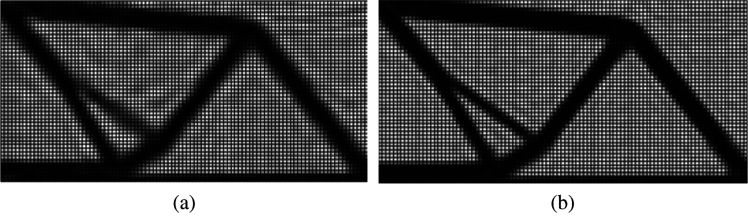
Figure 8: PGD based topology design. (a) Optimized design with 11 density modes (b) Optimized design with 19 density modes

Figure 9: Comparison of FEM-TO and PGD-TO results for a half MBB beam. (a) FEM-TO (b) PGD-TO

4.3 Parametric Learning and Uncertainty Quantification for Additive Manufacturing

Metal additive manufacturing is considered as the manufacturing technology of the future. However, design and development of additively manufactured metallic part is thwarted by the highly non-equilibrium nature of the process and resulting microstructure. The variable nature of the microstructure at different locations in the part gives rise to uncertainty in the resulting mechanical properties. The process conditions also result in residual stress inside the part, which is controlled by the microstructure as well. In turn, the residual stress will affect the microstructural feature such as the grain formation and dislocation distribution. The porosity formed during the manufacturing process is another concern in additive manufacturing. These microstructural features are the determining factors or parameters for the final mechanical properties such as the ultimate tensile strength or fatigue crack incubation life. The microstructural features are dependent on various process parameters such as scan speed, laser power, hatch spacing, powder composition, etc. The process-structure-property chain development by computational aid requires a method that can efficiently compute the field (thermal and mechanical) quantities for a large number of parameters. The proposed reduced order machine learning FEM framework has an immense prospect in this regard.

The outline of the application in the context of additive manufacturing is shown in Fig. 10. The AM-CFD [25] is the computational fluid dynamics code that can faithfully simulate the manufacturing process as a function of different process input parameters. This code can be extended with HiDeNN-FEM concept. The thermal history coming from the AM-CFD can be combined with HiDeNN-ROM to compute the residual stress field. Fig. 11 illustrates an example of residual stress obtained by an advanced ROM [42], which agrees well with the FEM solution. The final computed residual stress in terms of, e.g., two input parameters and locations (different material points) can be written in the following form:

σres(x,μ1,μ2)≈∑q=1Qux(q)(x)uμ1(q)(μ1)uμ2(q)(μ2)(35)

Here, σres is the residual stress, x is the material point, and μ1,μ2 are two manufacturing parameters. The resulting outcome (time-temperature history and residual stress) can be related to the microstructural features and different underlying physical phenomena. For example, the time temperature data holds the information coming from different time scales: nano to millisecond (meltpool dynamics), millisecond (scan speed), second (convection and radiation cooling and residual stress evolution). One way of relating this time-temperature history with mechanical properties is to apply feature engineering such as wavelet transformation and convolutional neural network [43]. In order to use these data-science tools, we need a large high fidelity database that can be generated quickly with the proposed HiDeNN-ROM.

Figure 10: A schematic diagram showing the potential application of HiDeNN-ROM to metal additive manufacturing. The time-temperature history contains multi-resolution information embedded. This multi-resolution time-temperature history and residual stress data can be obtained from the HiDeNN-ROM

Figure 11: Additive manufacturing residual stress obtained by FEM and advanced ROM [42]. (a) FEM (b) Advanced ROM

4.4 Multi-Physics Problems: Field Interaction Modeling of Robotic Materials

The multiphysics problems involves a large number of parameters that need to be considered for optimization, uncertainty quantification, and design. These challenging problems can be addressed by the proposed HiDeNN-PGD and HiDeNN-ROM.

Robotic materials are a class of multifunctional materials that combines responses from different physical field interactions to achieve desired functions. Earlier robotic materials were fabricated using soft matter that exhibited highly nonlinear behavior under the influence of environmental factors such as temperature, pressure, magnetic, electric, and optical fields [44]. Later research with soft robotic materials pushed their limits by considering inclusions of 2D materials or nanofillers, expanding the problem in multiple length scales. By design, these materials need to interact with external stimuli to attain necessary functionality. Therefore, the analysis needs to consider numerous design iterations involving solutions of multiple physical field interactions. In such scenarios, the use of conventional FEA methods is costly and a hindrance to effectively iterate through multiple length scales and multiple field interactions. The proposed HiDeNN-ROM framework can potentially handle the challenge of dimensional reduction by—first optimizing the nodal positions smartly and thus promoting the essence of r and h adaptivity [32], and secondly decoupling the field solvers in an attempt to accelerate the solution techniques using separation of variations as introduced in this work. After solving the problem, the field responses can assist in engineering the configuration for required functionality.

5  Conclusion

This paper proposes a new type of numerical method for analyzing the partial differential equations in computational science and engineering. The so-called reduced order machine learning FEM is a combination of scientific machine learning methods and model reduction techniques. We introduce a particular type of this method, called HiDeNN-PGD, which is actually a combination of HiDeNN-FEM and PGD based model reduction. Advantages of this synergy in accuracy and computational efficiency have been shown with an example of Poisson problems. It is found the HiDeNN-PGD is more accurate with a few modes than FEM and PGD. The potential applications of such method to real life problems have been discussed. We propose a well designed structure of the general HiDeNN-ROM for 1) the multi-scale analysis of composite materials, 2) topology optimization, 3) additive manufacturing. In particular, preliminary numerical results based on PGD-topology optimization have been reported for the first time. It is found that the proposed framework has a good potential to enable high resolution topology optimization at a significantly reduced cost. Finally, the application of the proposed method to multiphysics problems: the field interaction modeling of robotic materials, has also been discussed. We believe that the proposed reduced order machine learning FEM framework is a general and powerful tool for analyzing a large class problems with a high dimensional nature.

Acknowledgement: The authors would like to acknowledge the support of the National Science Foundation under Grant Nos. CMMI-1762035 and CMMI-1934367 and AFOSR under Grant No. FA9550-18-1-0381.

Funding Statement: WKL, YL, HL, SS, SM, AAA are supported by NSF Grants CMMI-1934367 and 1762035. In addition, WKL and SM are supported by AFOSR, USA Grant FA9550-18-1-0381.

Conflicts of Interest: The authors declare that they have no conflicts of interest to report regarding the present study.

This work is licensed under a Creative Commons Attribution 4.0 International License, which permits unrestricted use, distribution, and reproduction in any medium, provided the original work is properly cited.