| Computer Modeling in Engineering & Sciences |
DOI: 10.32604/cmes.2022.016857
ARTICLE
Estimation of Aleatory Randomness by Sa(T1)-Based Intensity Measures in Fragility Analysis of Reinforced Concrete Frame Structures
1College of Civil Engineering, Nanjing Forestry University, Nanjing, 210037, China
2Arup International Consultants (Shanghai) Co., Ltd., Shanghai, 200031, China
3College of Civil and Transportation Engineering, Hohai University, Nanjing, 210098, China
4Power China Huadong Engineering Corporation Limited (HDEC), Hangzhou, 311122, China
*Corresponding Author: Yantai Zhang. Email: atai1991@njfu.edu.cn
Received: 02 April 2021; Accepted: 07 July 2021
Abstract: Based on the multiple stripes analysis method, an investigation of the estimation of aleatory randomness by Sa(T1)-based intensity measures (IMs) in the fragility analysis is carried out for two typical low- and medium-rise reinforced concrete (RC) frame structures with 4 and 8 stories, respectively. The sensitivity of the aleatory randomness estimated in fragility curves to various Sa(T1)-based IMs is analyzed at three damage limit states, i.e., immediate occupancy, life safety, and collapse prevention. In addition, the effect of characterization methods of bidirectional ground motion intensity on the record-to-record variability is investigated. It is found that the damage limit state of the structure has an important influence on the applicability of the ground motion IM. The Sa(T1)-based IMs, considering the effect of softened period, can maintain lower record-to-record variability in the three limit states, and the Sa(T1)-based IMs, considering the effect of higher modes, do not show their advantage over Sa(T1). Furthermore, the optimal multiplier C and exponent α in the dual-parameter ground motion IM are proposed to obtain a lower record-to-record variability in the fragility analysis of different damage limit state. Finally, the improved dual-parameter ground motion IM is applied in the risk assessment of the 8-story frame structure.
Keywords: RC frame structure; intensity measure; fragility analysis; record-to-record variability; softened period; risk assessment
Reinforced concrete (RC) frame structures, as a structural system that enables flexible space separation, are widely used in Chinese cities. Previous earthquake damage surveys have shown that reinforced concrete frame structures are often severely damaged or even collapse during earthquakes [1–4]. Therefore, accurate and solid seismic fragility analysis of RC frame structures is important and necessary. Seismic fragility analysis is an effective method for evaluating the seismic performance of a structure from a probabilistic perspective [5–10].
The first and important step in the fragility analysis is to select a ground motion intensity measure (IM) to measure the aleatory randomness caused by record-to-record variability. The seismic IM is used as an intermediate variable to connect the seismic hazard and engineering performance demand measure (DM). To date, a variety of ground motion IMs have been proposed, and the selection of IMs depends not only on the structural system concerned but also on the engineering performance DM of interest [11–15]. Existing studies are mainly focused on the macro analysis of the relationship between ground motion IMs and engineering performance DMs. At the same time, the applicability of different IMs for seismic fragility analysis at various damage limit states has not yet been analyzed in depth.
The seismic fragility curve illustrates a structure's probability of exceeding a particular damage state under the action of earthquakes with different intensities. However, the establishment of fragility curves requires a significant amount of computations. Therefore, it is critical to quickly and easily estimate fragility curves. Commonly used methods for establishing fragility curves are incremental dynamic analysis [16–20], truncated incremental dynamic analysis [21], multiple stripes analysis [22,23], and static pushover analysis methods [24–26]. Compared with incremental dynamic analysis, the multiple stripes analysis method does not need to scale the amplitude of all the ground motions to a level that causes the damage limit state of interest, but only needs to analyze the structure at specific ground motion intensity levels [21]. The multiple stripes analysis method is equivalent to a special case of the IDA method. Even compared with the truncated incremental dynamic analysis, the calculation amount of the multiple stripes analysis is still smaller [21]. The multiple stripes analysis method can consider the influence of high-modes characteristics of high-rise structures and the hysteretic characteristics of structural members compared with static pushover analysis methods. Therefore, the multiple stripes analysis method can easily present the fragility curves while ensuring accuracy compared to other methods.
Spectral acceleration at fundamental period Sa(T1), a convenient and efficient intensity measure for first mode dominated structures [27], has been widely adopted in seismic design codes and research in many countries. In recent years, various forms of IMs have been proposed based on Sa(T1). The purpose of this paper is to investigate the estimation of aleatory randomness by using different Sa(T1)-based ground motion IMs in the fragility analysis in terms of different damage limit states for the RC frame structures. With thirty pairs of far-field records, multiple stripes analysis is carried out for two RC frame structures with 4 and 8 stories to explore the effect of Sa(T1)-based IMs on the record-to-record variability estimated in fragility curves of different damage limit states. The influence of the bidirectional ground motion intensity characterization methods on the seismic fragility assessment is also explored. Furthermore, the optimal parameters in the dual-parameter ground motion IM for the fragility analysis at different damage states are proposed through parameter analysis. Finally, the improved dual-parameter ground motion IM is applied to the risk assessment of exceeding each limit state for the 8-story frame structure according to the Chinses seismic code.
2 Sa(T1)-Based Ground Motion Intensity Measures
There are many types of ground motion IMs, and the application scopes of different ground motion IMs are different [11,12]. Due to the structural characteristics of RC frame structures, frame buildings in seismic high-risk areas are often structurally not high, and then their dynamic characteristics are generally dominated by the first vibration mode. The spectral acceleration at the first vibration period Sa(T1) is a convenient and efficient ground motion IM in the seismic analysis of structures dominated by the first mode [27]. However, RC frame structures are prone to be elasto-plastic under the action of strong earthquakes, and a single Sa(T1) cannot reflect this characteristic. Cordova et al. [28] considered the effect of structural stiffness degradation and proposed the dual-parameter ground motion IM S* (see Table 1), where the softened period Tf = 2T1 and the combination coefficient α = 0.5. Mehanny [29] proposed the improved IM-CR and IM-SR based on S*. By introducing the self-adaptive parameter RIM, both IM-CR and IM-SR can be applied to situations with different nonlinear levels. RIM was recommended to be 2. Bojórquez et al. [30] proposed an IM exploring the geometric mean of spectral acceleration at multiple periods, in which the parameter Np is used to capture the spectral shape, and TN = 2T1 and α = 0.4 are recommended.
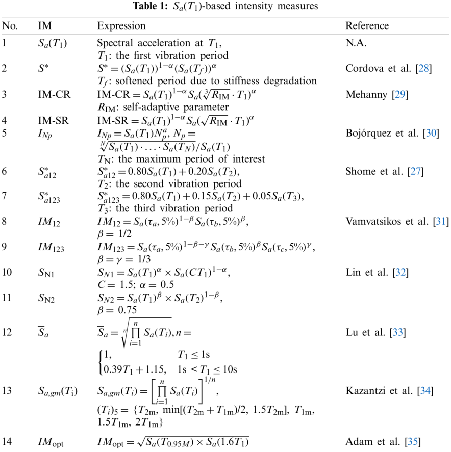
However, the abovementioned ground motion IMs only capture the effect of period elongation and do not reflect the effect of higher vibration modes for long-period structures. Some studies have pointed out that ground motion IMs considering the higher vibration mode are suitable for high-rise buildings. The linear combination-type IMs
Two typical 4- and 8-story RC frame structures with seismic design [36,37] according to the current Chinese Code for Seismic Design of Building [38] are selected as the analysis cases, as shown in Fig. 1. The total heights of the building are 16.2 and 31.8 m, respectively, of which the height of the first story is 4.5 m and the other layers are 3.9 m. The typical floor plan of those buildings is shown in Fig. 2. The frames belong to the seismic precautionary building of Category-C with a design precautionary intensity of 8. Both frames belong to the first design earthquake group, and have type II site classification. The roof dead load and live load are set as 7 and 0.7 kN/m2, respectively. The floor dead and live load are taken as 5 and 2 kN/m2. The load of the infill wall is evenly distributed on the beam, 6 kN/m for the outer wall and 3 kN/m for the inner wall. The frame beams and columns are made of C40 concrete, and the longitudinal reinforcement is HRB335. The detailed dimensions and reinforcement information of frame beams and columns can be found in Wang [36] and He et al. [37].
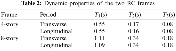
The two RC frames are modeled in the program OpenSEES developed by the Pacific Earthquake Engineering Research (PEER) center [39]. Concrete02 is used to describe the behavior of concrete, and Steel02 is used to represent the behavior of steel. Concrete02 can consider the tensile mechanical properties of concrete and the degradation of unloading stiffness [40]. Steel02 can reflect the isotropic hardening effect and the Bauschinger effect. It is very efficient in calculation because it uses the explicit function expression of strain, and at the same time it maintains good consistency with the results of the cyclical loading tests of steel bars [41]. Columns and beams are modeled by fiber dispBeamColumn elements, by which the nonlinear characteristics of components can be precisely simulated with a small calculation cost compared to standard beam finite elements in general-purpose engineering simulation software. From the aspect of material constitutive, one-dimensional material constitutive is enough for fiber dispBeamColumn elements. From the aspect of simulating deformation, fiber dispBeamColumn elements can simulate bending deformation and axial deformation well, and steel and concrete can be considered separately from the aspect of modeling. The P-delta effect is considered in the models, and Rayleigh damping is used herein with a damping ratio of 5% assumed. Table 2 summarizes some transverse and longitudinal vibration periods of the two RC frames. More detailed modeling information can be obtained referring to Wang [36] and He et al. [37].
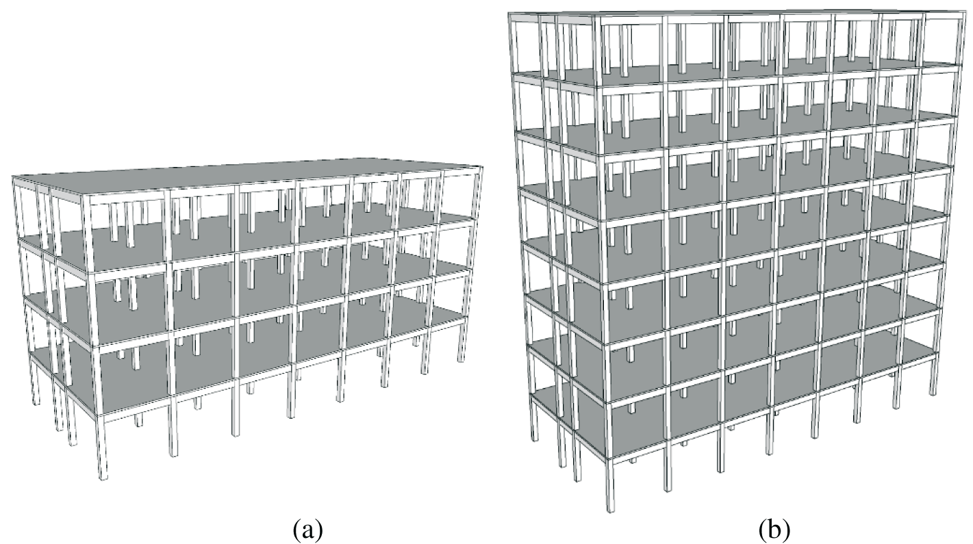
Figure 1: Three-dimensional model of the two RC frames (a) 4-story (b) 8-story
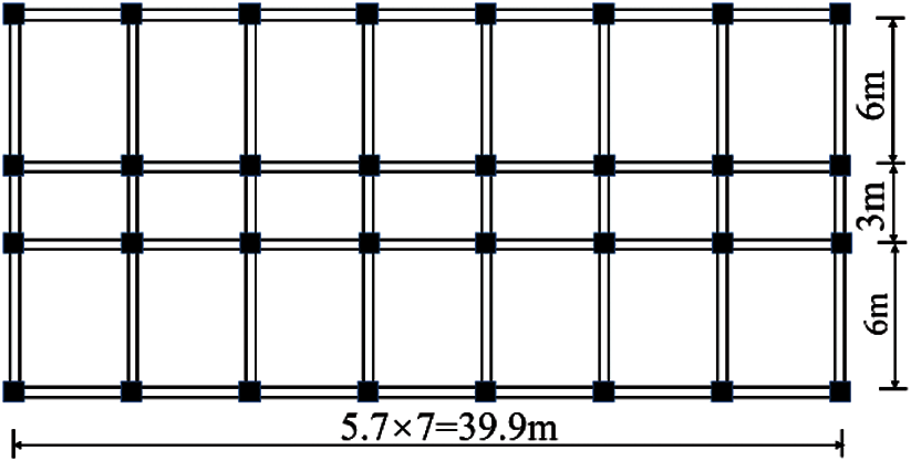
Figure 2: Typical floor plan of the two RC frame structures
3.2 Selection of Ground Motions
Thirty pairs of far-field ground motions (see Table 3) are selected here from the PEER strong motion database [42–44] according to the selection criteria recommended in FEMA P695 [45]. The source-to-distance of the far-field ground motions is greater than 10 km, and enough records from large-magnitude earthquake events are chosen to ensure record-to-record variability. The moment magnitudes of earthquakes are larger than 6.2 with a mean value of 7.0. PGA1 (PGA of Component 1) and PGA2 (PGA of Component 2) of the records are listed in Table 3. The average value of the maximum peak ground acceleration PGAmax of the two components is 0.46 g. The acceleration response spectra of the ground motions with a 5% damping ratio are illustrated in Fig. 3.
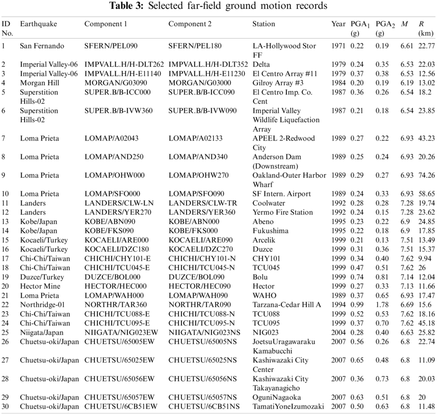
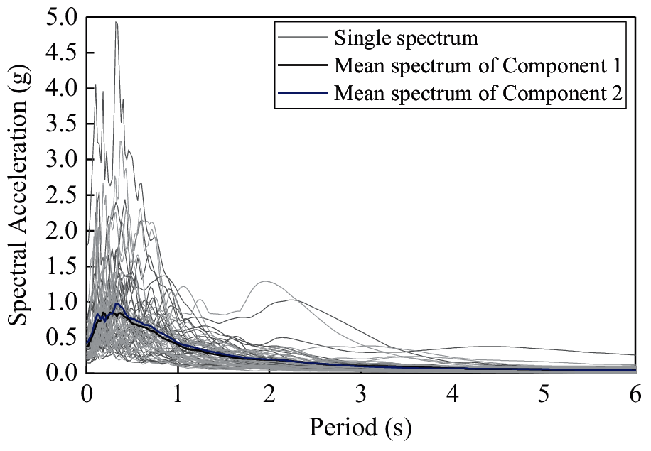
Figure 3: Acceleration response spectra of the selected records with 5% damping ratio
3.3 Multiple Stripes Analysis and Criteria for Each Damage Limit State
The multiple stripes analysis method is selected here to obtain the fragility curves at different damage limit states, as it does not need to scale all the ground motions to the IM levels that cause the damage limit state of interest. Beacuse multiple stripes analysis can only produce the fractions of the damage limit state at some IM levels, the maximum likelihood estimation method, an appropriate fitting approach for the multiple stripes analysis method, is utilized [5,21]. The seismic response from each ground motion is assumed to be independent of the results from other ground motions. The maxima of fragility curve parameters can be obtained by Eq. (1). A detailed introduction to the application of the fitting approach in multiple stripes analysis can be found in Baker [21].
where η is the median capacity at a specific limit state; βRTR is the lognormal standard deviation, which represents the record-to-record variability; m is the number of IM levels; Φ() is the standard normal cumulative distribution function; zj is the number of observations of the limit state out of nj ground motions in the case of intensity level IMj.
The bidirectional ground motions in Table 3 are applied to the two RC frames to obtain the fragility curves at different damage limit states by using multiple stripes analyses. Component 1 of the ground motions is applied to the transverse direction of the frames, and Component 2 is applied to the longitudinal direction. The amplitude scaling is based on Component 1, and the same scale factor is used for Component 2 to preserve the relative amplitude of the two components of the record. In the fragility analysis, the criteria of each damage limit state are determined according to FEMA 356 [46] as shown in Table 4. For the immediate occupancy (IO) limit state, the maximum inter-story drift ratio θmax of RC frames is set as 1%; for the life safety (LS) limit state, the ratio θmax is suggested as 2%; and for the collapse prevention (CP) limit state, the ratio θmax is set as 4%.
It should be noted that the number of IM levels m (see Eq. (1)) is a key parameter for the fitted results in the multiple stripes analysis. If the number of IM levels is larger, the computational cost increases, while if the number of IM levels is smaller, the accuracy of the results cannot be guaranteed. Eads et al. [47] found that the analysis result is mainly affected by the IM levels at the lower half of the fragility curve. Additionally, Baker [21] pointed out that the fragility function can be effectively estimated by the IM levels with a low probability. Héctor Dávalos et al. [48] recommended that it is better to conduct multiple stripes analyses at only two intensity levels, namely, enhanced two-stripe analysis (E2SA). Zhang et al. [44] suggested using three IM levels with two levels lower than the estimated median limit capacity in the multiple stripes analysis. In general, an accurate result can be obtained by the IM levels focused on the lower half of the fragility curve. Therefore, six IM levels with PGA1 (i.e., PGA of Component 1of the records) equal to 0.25, 0.35, 0.45, 0.85, 1.25 and 1.65 g are used in the multiple stripes analysis of the three fragility limit states in this paper. This strategy ensures that there are no less than two fraction points in the lower half of the fragility curves of the three limit states, as shown in Figs. 4 to 5.
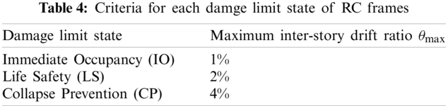
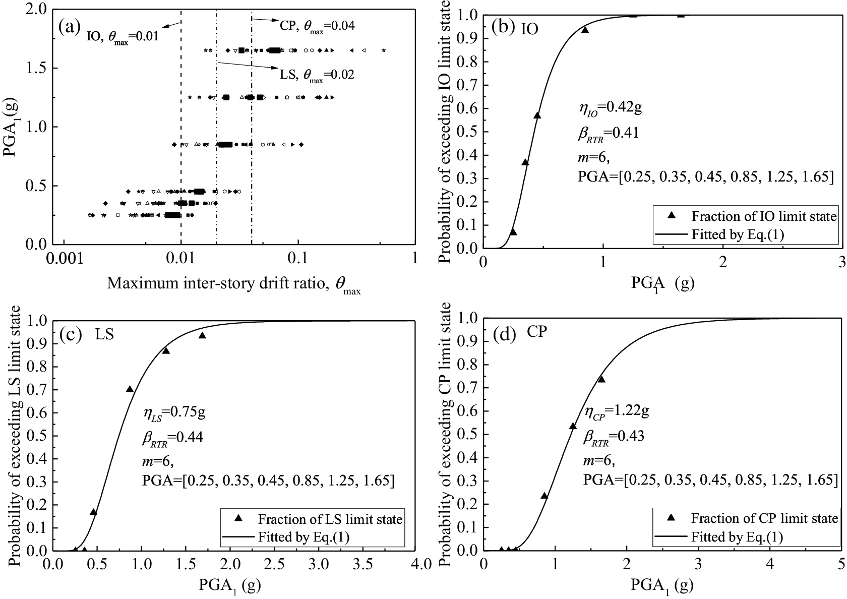
Figure 4: Fragility curves characterized by PGA1 for the 4-story building (a) maximum inter-story drift ratio θmax under different PGA1 levels; (b) fragility curve estimated for IO limit state; (c) fragility curve estimated for LS limit state; (d) fragility curve estimated for CP limit state
In Fig. 4, the median capacity at IO limit state ηIO for the 4-story building is 0.42, the median capacity at LS limit state ηLS is 0.75 g and the median capacity at CP limit state ηCP is 1.22 g. In Fig. 5, the median capacity at IO limit state ηIO for the 8-story building is 0.36 g, the median capacity at LS limit state ηLS is 0.72 g and the median capacity at CP limit state ηCP is 1.55 g. From the IO to CP limit states, the lognormal standard deviations βRTR increase from 0.41 to 0.44 and then to 0.43 in the case of the 4-story building. However, in the case of 8-story building, βRTR is 0.75, 0.57 and 0.61, which do not show a certain regularity. This may be caused by the characteristics of the building itself.
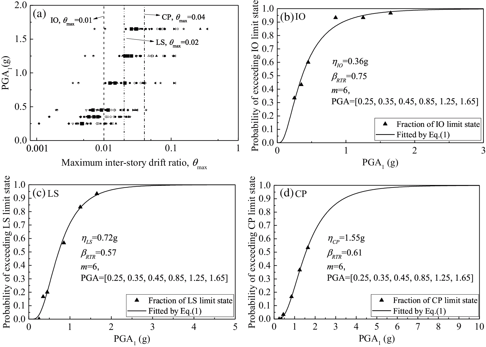
Figure 5: Fragility curves characterized by PGA1 for the 8-story building (a) maximum inter-story drift ratio θmax under different PGA1 levels; (b) fragility curve estimated for IO limit state; (c) fragility curve estimated for LS limit state; (d) fragility curve estimated for CP limit state
4 Estimation of Aleatory Randomness
In addition to the fourteen IMs listed in Table 1, three simple amplitude-type IMs PGA, peak ground velocity (PGV) and peak ground displacement (PGD) are also evaluated here. For S*, α is set as 0.5 and Tf is set to be 2T1. For IM-CR and IM-SR, α is set as 0.5 and RIM is taken as 2. In INp, TN is taken as 2T1 and α is set as 0.4. The original parameters in Table 1 are used in
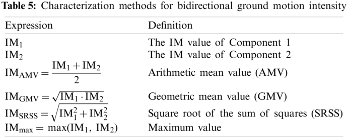
Lucchini et al. [49] and Kostinakis et al. [50] pointed out that the characterization methods of bidirectional ground motion intensity using a single value influence the correlation between the ground motion IMs and engineering performance DM. Therefore, the influence of different characterization methods on the record-to-record variability in the fragility analysis is also investigated herein. As shown in Table 5, six characterization methods for bidirectional ground motion intensity are used here [50].
It should be noted that each ground motion has a different IM level when using different characterization methods or IMs other than PGA1. In such a situation, to estimate the fragility curves, njin Eq. (1) is set to 1, and the probability of a particular limit state is set to 1 if θmax is larger than the corresponding criterion. Taking Sa(T1) as an example, the analysis processes of the 4-story frame using the two bidirectional characterization methods, i.e., IM1 and IMSRSS, are shown in Figs. 6 and 7, respectively. Figs. 6 and 7 show that βRTR estimated by Sa(T1) increases roughly with the shift of the limit state from IO to CP in both the bidirectional ground motion intensity characterization methods IM1 and IMSRSS.
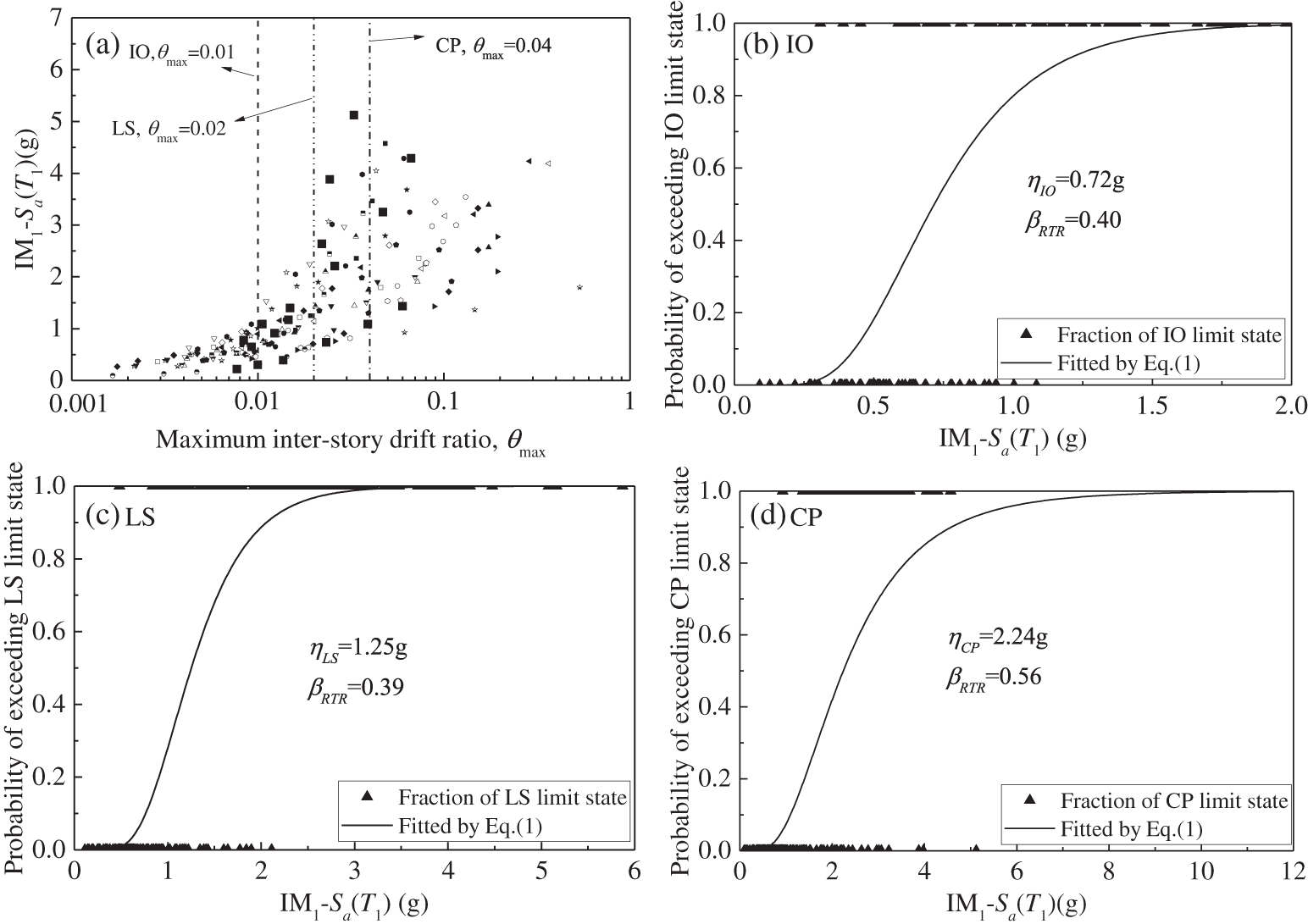
Figure 6: Fragility curves characterized by Sa(T1) in the case of IM1 for the 4-story frame (a) maximum inter-story drift ratio θmax under different IM1-Sa(T1)) levels; (b) fragility curve estimated for IO limit state; (c) fragility curve estimated for LS limit state; (d) fragility curve estimated for CP limit state
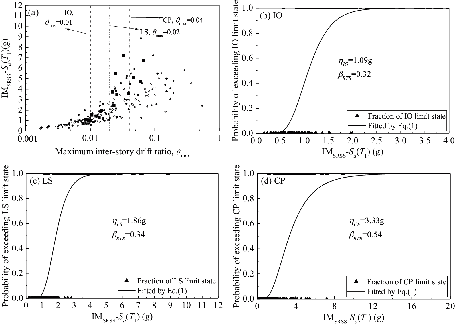
Figure 7: Fragility curves characterized by Sa(T1) in the case of IMSRSS for the 4-story frame (a) maximum inter-story drift ratio θmax under different IMSRSS-Sa(T1) levels; (b) fragility curve estimated for IO limit state; (c) fragility curve estimated for LS limit state; (d) fragility curve estimated for CP limit state
Figs. 8 to 9 illustrate the uncertainties of the ground motion βRTR estimated in three limit states of the two buildings using different bidirectional characterization methods. It can be seen from the figures that the limit state of the structure has an important influence on the applicability of the ground motion IM. With the development of the damage state, that is, from the IO limit state to the CP limit state, the uncertainties of the ground motion βRTR corresponding to each IM generally show an increasing trend.
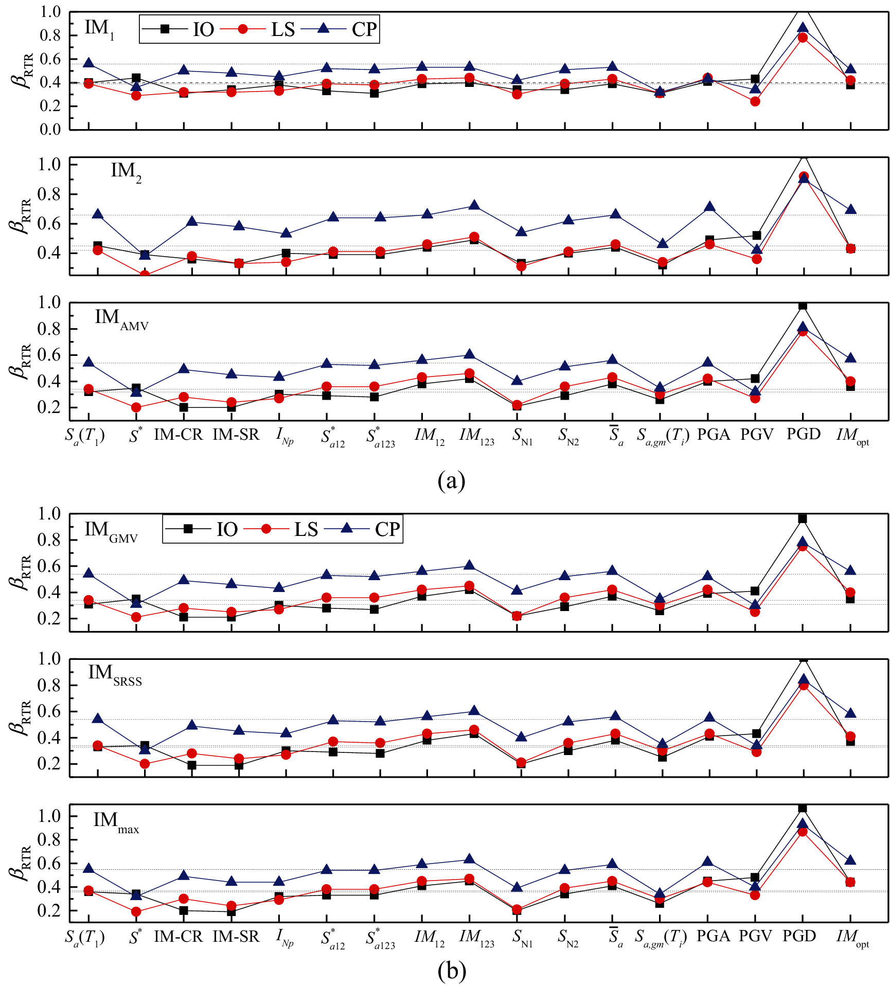
Figure 8: Record-to-record variability βRTR estimated in fragility analysis of the three limit states for the 4-story building by using six bidirectional characterization methods (a) IM1, IM2 and IMAMV (b) IMGMV, IMSRSS and IMmax
For both 4- and 8-story buildings, the IMs considering the effect of higher modes, such as
With respect to most bidirectional characterization methods, both dual-parameter IMs S* and SN1 can maintain lower βRTR in the three limit states for the two buildings. Although IM-CR, IM-SR and INP are also combination-type ground motion IMs that consider the effect of period elongation, their differences in the selected softened period or the power exponents from S* and SN1 caused significant differences in the evaluation of ground motion uncertainty. It is worth noting that in the IO state, the βRTR of SN1, IM-CR and IM-SR is smaller than S*. The selected softened periods in SN1, IM-CR and IM-SR are smaller than that of S*. This shows that the selected softened period should not be a fixed value in different damage states. As analyzed, when the appropriate softened period is selected, that is, the appropriate parameter C in Tf = CT1, the smallest βRTR can be obtained. For the three amplitude-type IMs, PGV has apparent advantages in the three limit states of the buildings. Although IMopt considered the impact of the number of floors in the structure, its performance is not satisfactory, which may be due to the failure to consider the fundamental period of the structure.
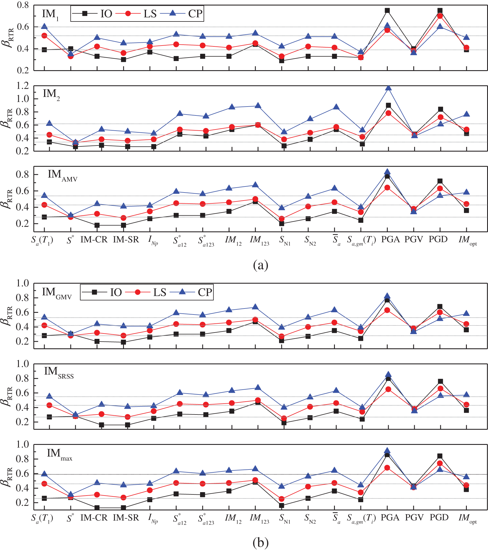
Figure 9: Record-to-record variability βRTR estimated in fragility analysis of the three limit states for the 8-story building by using six bidirectional characterization methods (a) IM1, IM2 and IMAMV (b) IMGMV, IMSRSS and IMmax
The uncertainties estimated by a specific IM using different bidirectional ground motion intensity characterization methods are different, as shown in Figs. 8 and 9. It can be seen from the above analysis that S* and SN1 have apparent advantages in estimating of the uncertainty of ground motion. Taking S* and SN1 as examples, the βRTR estimated in the six bidirectional characterization methods are illustrated in Figs. 10 and 11, respectively. Since only one direction of ground motion intensity is considered, there is a large difference between IM1 and IM2. Structural damage may be related to the intensity of ground motion in both directions. When considering the combination of the intensity in the two directions, IMAMV, IMGMV and IMSRSS can predict relatively stable and similar βRTR in the two structures for each limit state. The βRTR obtained by the two methods is close to the minimum in most cases.
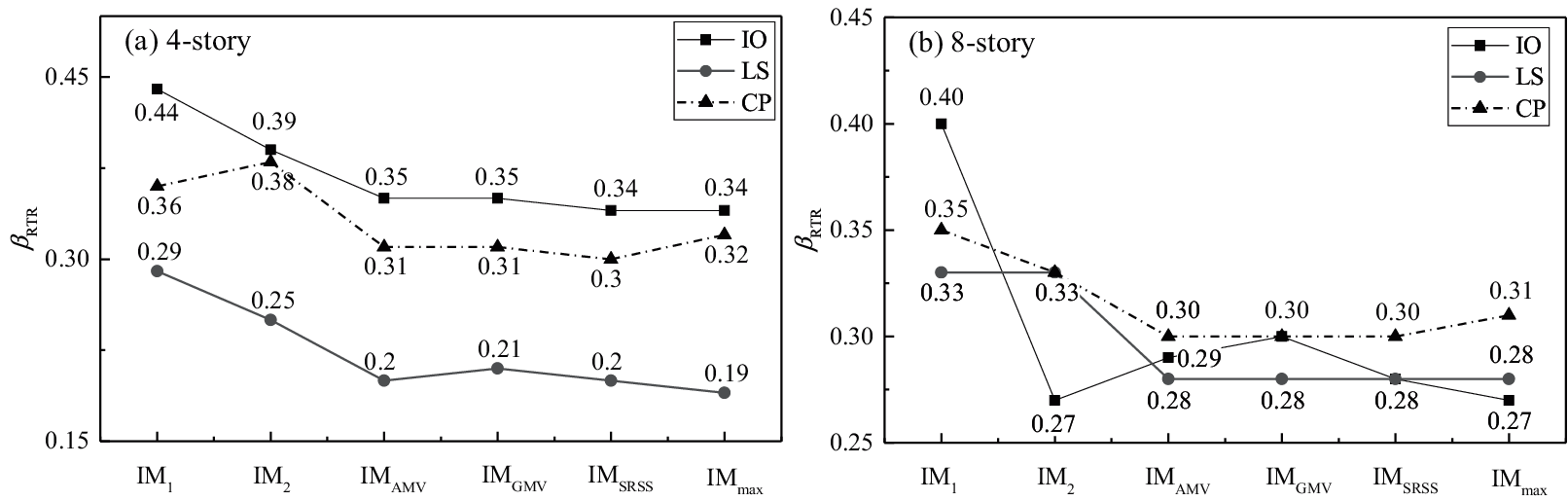
Figure 10: βRTR estimated by S* with the six bidirectional characterization methods
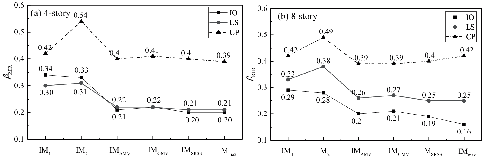
Figure 11: βRTR estimated by SN1 with the six bidirectional characterization methods
5 Improved IM for Fragility Analysis at Different Limit States
From the analysis in the previous section, it can be concluded that the selected softened period in the dual-parameter IM (see Eq. (2)) should not be a fixed value in different damage states. As analyzed, when the appropriate softening period is selected, that is, parameter C in Tf = CT1 as listed in Eq. (2), a smaller βRTR can be obtained. Shown in Fig. 12 are the βRTR estimated by the spectral acceleration at any vibration period of interest. It should be noted that the geometric mean value IMGMV is used here to consider the bidirectional ground motion intensities. Obviously, in the fragility analysis at the three limit states, all the minimum βRTR values are achieved at the softened period in the three structures. As the damage intensifies, the point where the minimum βRTR is obtained moves to the right. As shown in the figure, the point of obtaining the minimum βRTR moves from position A to position B and finally moves to position C from IO to LS and then to CP. That is, as the damage intensifies, the spectral acceleration at a longer softened period has a better correlation with structural damage, namely, a smaller dispersion is achieved. The softened period Tf in Eq. (2) should be adjusted according to the damage limit state of the structure in the fragility analysis.
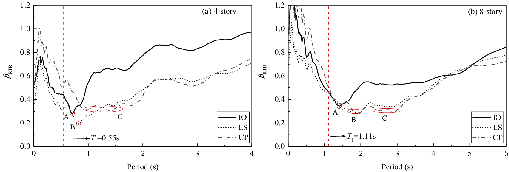
Figure 12: βRTR estimated by the spectral acceleration at any vibration period for the three limit states
In addition, Fig. 12 shows that the spectral acceleration corresponding to the higher modes often achieves a higher βRTR, which is why the IMs considering the effect of higher modes do not perform well, as analyzed in the previous section. Studies have shown that the spectral acceleration corresponding to the higher modes can achieve a higher correlation with structural damage in super high-rise buildings [33,43].
5.2 Optimal C and α in Dual-Parameters IM
In this section, the optimal multiplier C and exponent α suitable for fragility analysis at different damage limits are suggested through parameter analysis. Figs. 13 to 14, presented in the form of contour maps, illustrate the influence of different combinations of C and α on standard deviations, βRTR. The blue part depicts a smaller value of βRTR, and the red part depicts a larger value of βRTR. Note that the geometric mean value IMGMV is used here to reflect the bidirectional ground motion intensity.
Under different combinations of C and α, the lognormal standard deviations βRTR are different and reflect apparent regularity. The optimal combination of the parameters, C and α, is determined when βRTR reaches its minimum. It can be seen from the figure that the position of the smaller dispersion βRTR (see the blue part) is shifted to the right part with a larger C as the damage increases in each structure. That is, structural damage has a better correlation with a longer softening period from the IO limit state to the CP limit state. In addition, the position to achieve a smaller dispersion βRTR moves downward, especially from the IO limit state to the LS limit state. That is, the weight of the softened period, i.e., the combination coefficient α in the IM, is decreasing.
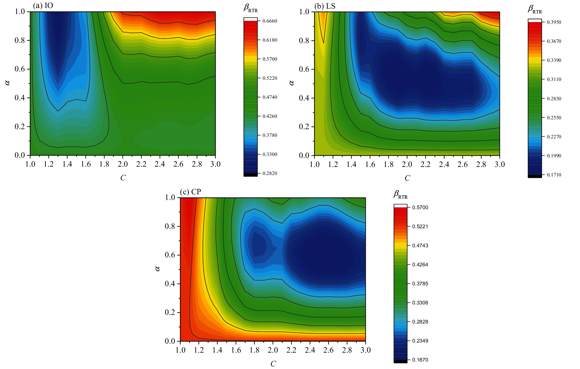
Figure 13: Relation between βRTR and C, α for the 4-story building
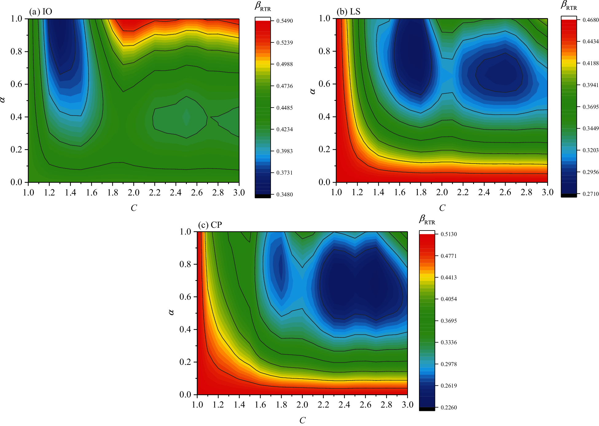
Figure 14: Relation between βRTR and C, α for the 8-story building
Table 6 lists the ranges of C and α by which the two structures can achieve relatively smaller dispersion βRTR under the three limit states. As seen from the table, the value of C increases from IO to CP. In addition, α is getting smaller, especially from IO to LS. Thus, to achieve analytical simplicity, for the IO state, it is recommended to set α to 0.9 and C to 1.3; for the LS state, it is recommended to set α to 0.7 and C to 1.8; for the CP state, it is recommended to set α to 0.6 and C to 2.4, as shown in the improved IM
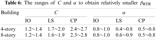
Fig. 15 shows the dispersion βRTR estimated with the improved IM by adopting the parameters suggested in Eq. (3). Compared with S* and SN1 (see Figs. 10 and 11), the improved IM
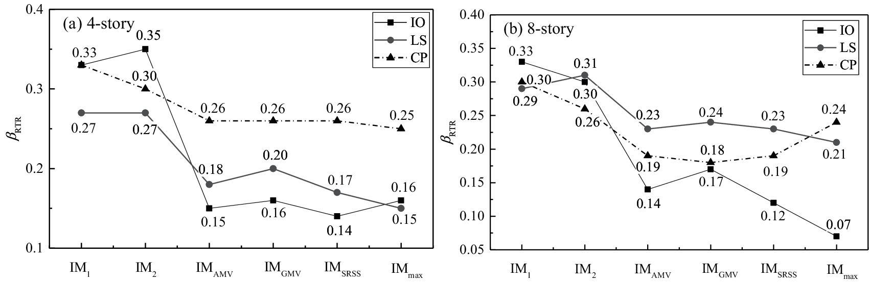
Figure 15: βRTR estimated by
6 Risk Assessment by the Improved IM
In this section, the improved IM is further applied to the risk assessment at the three limit states for the 8-story frame structure according to Chinese codes. Generally, the fragility curve corresponding to one limit state is assumed to be a lognormal cumulative distribution function (see Eq. (4)) as used above in Eq. (1).
where
where k0 and k are two empirical factors. These Sa(T1) and Sa(Tf) corresponding to the frequent earthquake (63.2% probability of exceedance in 50 years), the design basis earthquake (10% probability of exceedance in 50 years) and the maximum considered earthquake (2% probability of exceedance in 50 years) are obtained referring to the Code for Seismic Design of Buildings [38] for the regions with seismic precautionary intensity of 8. Then, the
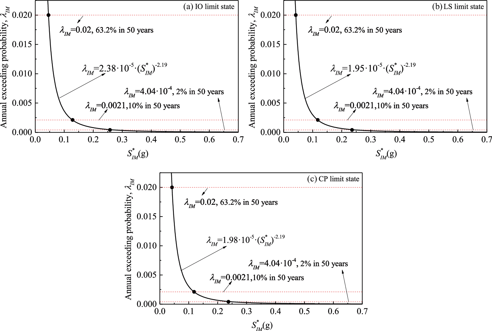
Figure 16: Mean hazard curves expressed by
The annual probability of exceeding one specific limit state, as listed in Eq. (6), can be obtained through the total probability theory by combining the fragility curve (Eq. (4)) with the seismic hazard curve (Eq. (5)).
Furthermore, Eq. (7) can be obtained by substituting and simplifying Eq. (6) [52]. It should be noted that there is no consideration of epistemic uncertainty in Eq. (7).
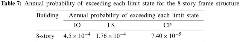
Table 7 shows the annual probability of exceeding each limit state for the 8-story frame structure. Note that the median capacity η and lognormal standard deviation βRTR are estimated by
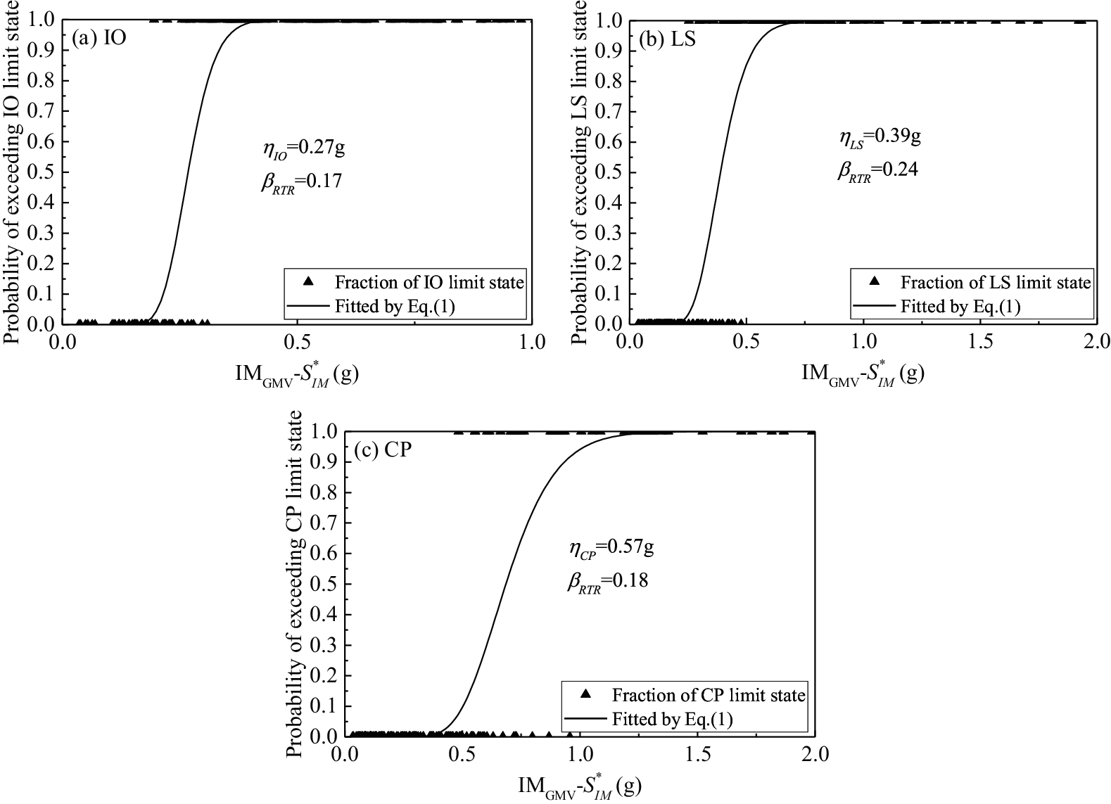
Figure 17: Fragility curves characterized by
Based on two low- and medium-rise RC frame structures, an investigation is first provided in this study regarding the estimation of record-to-record variability βRTR by using Sa(T1)-based IMs in the fragility curves of three limit states (i.e., IO, LS and CP). Subsequently, the optimal multiplier C and exponent α in the dual-parameter IM for different limit states are suggested through parameter analysis. Furthermore, the improved dual-parameter IM is applied to the risk assessment at the three limit states. Several observations can be reached from the case study on the RC frame structure, as follows:
(1) The limit state of the structure has an important influence on the applicability of Sa(T1)-based IMs. From the IO limit state to the CP limit state, the uncertainties of the ground motion βRTR corresponding to most IMs generally show an increasing trend. For low- and medium–rise RC frame structures, the Sa(T1)-based IMs considering the effect of a softened period, i.e., S* and SN1, can maintain a lower βRTR in the three limit states compared to the Sa(T1)-based IMs considering the effect of higher modes.
(2) With increasing structural damage, spectral acceleration and structural damage have a better correlation at longer softening period. The selected softened period in the dual-parameter IM should not be a fixed value in different damage states. In addition, as the damage develops, the combination index α in dual-parameter IM should be reduced to obtain a better correlation. Taking into account the different damage states, a dual variable-parameter is adopted in the improved IM.
(3) The record-to-record variability estimated using different bidirectional ground motion intensity characterization methods with respect to a specific IM is continually varying. The characterization method that only considers the intensity of ground motion in a single direction, IM1 or IM2, lacks stability. When considering the combination of the intensity in the two directions, IMAMV, IMGMV and IMSRSS can predict relatively stable and similar βRTR. By adopting IMGMV, the annual probabilities of exceeding each limit state for the 8-story frame structure were analyzed.
Only two typical low- and medium-rise frame buildings with 4 and 8 stories are employed here. In addition, only 30 pairs of far-field records are selected in this paper. More structure cases and ground motion records with different spectral characteristics, such as near-field records, are needed to verify the suggested parameters in the improved IM.
Funding Statement: This research was financially supported by the Jiangsu Youth Fund Projects (SBK2021044269), the National Natural Science Foundation of China Youth Fund (52108457, 52108133), the Natural Science Foundation of the Jiangsu Higher Education Institutions of China (20KJB560014), Fundamental Research Funds for the Central Universities (B210201019), High-level Talent Research Fund of Nanjing Forestry University (163050115), Nanjing Forestry University Undergraduate Innovation Training Program (2021NFUSPITP0221, 2020NFUSPITP0352 and 2020NFUSPITP0373), and Jiangsu Undergraduate Innovation Training Program (202110298079Y).
Conflicts of Interest: The authors declare that they have no conflicts of interest to report regarding the present study.
1. Ye, L. P., Lu, X. Z., Zhao, S. C., Li, Y. (2009). Seismic collapse resistance of RC frame structures-case studies on seismic damages of several RC frame structures under extreme ground motion in Wenchuan earthquake. Journal of Building Structures, 30(6), 67–76 (in Chinese). DOI 10.14006/j.jzjgxb.2009.06.009. [Google Scholar] [CrossRef]
2. Huo, L. S., Li, H. N., Xiao, S. Y., Wang, D. S. (2009). Earthquake damage investigation and analysis of reinforced concrete frame structures in Wenchuan earthquake. Journal of Dalian University of Technology, 49(5),718–723 (in Chinese). [Google Scholar]
3. Huang, L., Zhou, Z., Liu, H., Si, Y. (2021). Experimental investigation of hysteretic performance of self-centering glulam beam-to-column joint with friction dampers. Journal of Earthquake and Tsunami, 15(1), 2150005. DOI 10.1142/S1793431121500056. [Google Scholar] [CrossRef]
4. Huang, L., Zhou, Z., Clayton, P. M. (2021). Experimental and numerical study of unbonded post-tensioned precast concrete connections with controllable post-decompression stiffness. The Structural Design of Tall and Special Buildings, 30(7), e1847. DOI 10.1002/tal.1847. [Google Scholar] [CrossRef]
5. Shinozuka, M., Feng, M. Q., Lee, J., Naganuma, T. (2000). Statistical analysis of fragility curves. Journal of Engineering Mechanics, 126(12), 1224–1231. DOI 10.1061/(ASCE)0733-9399(2000)126:12(1224). [Google Scholar] [CrossRef]
6. Moehle, J., Deierlein, G. G. (2004). A framework methodology for performance-based earthquake engineering. Proceedings of the 13th World Conference on Earthquake Engineering, Vancouver, B.C., Canada. [Google Scholar]
7. Li, G., Dong, Z. Q., Li, H. N., Yang, Y. B. (2017). Seismic collapse analysis of concentrically-braced frames by the IDA method. Advanced Steel Construction, 13(3), 273–293. DOI 10.18057/IJASC.2017.13.3.5. [Google Scholar] [CrossRef]
8. Fu, X., Li, H. N., Li, G., Dong, Z. Q. (2020). Fragility analysis of a transmission tower under combined wind and rain loads. Journal of Wind Engineering & Industrial Aerodynamics, 199, 104098. DOI 10.1016/j.jweia.2020.104098. [Google Scholar] [CrossRef]
9. Kassem, M. M., Nazri, F. M., Farsangi, E. N. (2020). The efficiency of an improved seismic vulnerability index under strong ground motions. Structures, 23, 366–382. DOI 10.1016/j.istruc.2019.10.016. [Google Scholar] [CrossRef]
10. Kassem, M. M., Nazri, F. M., Wei, L. J., Tan, C. G., Shahidan, S. et al. (2019). Seismic fragility assessment for moment-resisting concrete frame with setback under repeated earthquakes. Asian Journal of Civil Engineering, 20(3), 465–477. DOI 10.1007/s42107-019-00119-z. [Google Scholar] [CrossRef]
11. Riddell, R. (2007). On ground motion intensity indices. Earthquake Spectra, 23(1), 147–173. DOI 10.1193/1.2424748. [Google Scholar] [CrossRef]
12. Ye, L. P., Ma, Q. L., Miao, Z. W., Zhuge, Y. (2013). Numerical and comparative study of earthquake intensity indices in seismic analysis. The Structural Design of Tall and Special Buildings, 22(4), 362–381. DOI 10.1002/tal.693. [Google Scholar] [CrossRef]
13. Ebrahimian, H., Jalayer, F., Lucchini, A., Mollaioli, F., Manfredi, G. (2015). Preliminary ranking of alternative scalar and vector intensity measures of ground shaking. Bulletin of Earthquake Engineering, 13(10), 2805–2840. DOI 10.1007/s10518-015-9755-9. [Google Scholar] [CrossRef]
14. Kostinakis, K., Fontara, I. K., Athanatopoulou, A. M. (2018). Scalar structure-specific ground motion intensity measures for assessing the seismic performance of structures: A review. Journal of Earthquake Engineering, 22(4), 630–665. DOI 10.1080/13632469.2016. 1264323. [Google Scholar] [CrossRef]
15. Zhang, Y. T., He, Z. (2019). Appropriate ground motion intensity measures for estimating the earthquake demand of floor acceleration-sensitive elements in super high-rise buildings. Structure and Infrastructure Engineering, 15(4), 467–483. DOI 10.1080/15732479.2018.1544986. [Google Scholar] [CrossRef]
16. Vamvatsikos, D., Cornell, C. A. (2002). Incremental dynamic analysis. Earthquake Engineering & Structural Dynamics, 31(3), 491–514. DOI 10.1002/eqe.141. [Google Scholar] [CrossRef]
17. Dolšek, M. (2009). Incremental dynamic analysis with consideration of modeling uncertainties. Earthquake Engineering & Structural Dynamics, 38(6), 805–825. DOI 10.1002/eqe. 869. [Google Scholar] [CrossRef]
18. Pang, R., Xu, B., Kong, X., Zou, D. (2018). Seismic fragility for high CFRDs based on deformation and damage index through incremental dynamic analysis. Soil Dynamics and Earthquake Engineering, 104, 432–436. DOI 10.1016/j.soildyn.2017.11.017. [Google Scholar] [CrossRef]
19. Pang, R., Xu, B., Zou, D., Kong, X. (2019). Seismic performance assessment of high CFRDs based on fragility analysis. Science China Technological Sciences, 62(4), 635–648. DOI 10.1007/s11431-017-9220-8. [Google Scholar] [CrossRef]
20. Pang, R., Xu, B., Zhou, Y., Zhang, X., Wang, X. (2020). Fragility analysis of high CFRDs subjected to mainshock-aftershock sequences based on plastic failure. Engineering Structures, 206, 110152. DOI 10.1016/j.engstruct.2019.110152. [Google Scholar] [CrossRef]
21. Baker, J. W. (2015). Efficient analytical fragility function fitting using dynamic structural analysis. Earthquake Spectra, 31(1), 579–599. DOI 10.1193/021113EQS025M. [Google Scholar] [CrossRef]
22. Jalayer, F. (2003). Direct probabilistic seismic analysis: Implementing non-linear dynamic assessments. Stanford University, Stanford, CA. [Google Scholar]
23. Jalayer, F., Cornell, C. A. (2009). Alternative non-linear demand estimation methods for probability-based seismic assessments. Earthquake Engineering & Structural Dynamics, 38(8), 951–972. DOI 10.1002/eqe.876. [Google Scholar] [CrossRef]
24. Dolšek, M. (2012). Simplified method for seismic risk assessment of buildings with consideration of aleatory and epistemic uncertainty. Structure and Infrastructure Engineering, 8(10), 939–953. DOI 10.1080/15732479.2011.574813. [Google Scholar] [CrossRef]
25. Fragiadakis, M., Vamvatsikos, D. (2010). Fast performance uncertainty estimation via pushover and approximate IDA. Earthquake Engineering & Structural Dynamics, 39(6), 683–703. DOI 10.1002/eqe.965. [Google Scholar] [CrossRef]
26. Han, S. W., Moon, K. H., Chopra, A. K. (2010). Application of MPA to estimate probability of collapse of structures. Earthquake Engineering & Structural Dynamics, 39(11), 1259–1278. DOI 10.1002/eqe.992. [Google Scholar] [CrossRef]
27. Shome, N., Cornell, C. A. (1999). Probabilistic seismic demand analysis of non-linear structures (Report No. RMS-35). Stanford University, Stanford, CA. [Google Scholar]
28. Cordova, P. P., Deierlein, G. G., Mehanny, S. S., Cornell, C. A. (2001). Development of a two-parameter seismic intensity measure and probabilistic assessment procedure. Proceedings of the Second US-Japan Workshop on Performance-Based Earthquake Engineering Methodology for Reinforced Concrete Building Structures. Sapporo, Japan. [Google Scholar]
29. Mehanny, S. S. (2009). A broad-range power-law form scalar-based seismic intensity measure. Engineering Structures, 31(7), 1354–1368. DOI 10.1016/j.engstruct.2009.02.003. [Google Scholar] [CrossRef]
30. Bojórquez, E., Iervolino, I. (2011). Spectral shape proxies and nonlinear structural response. Soil Dynamics and Earthquake Engineering, 31(7), 996–1008. DOI 10.1016/j.soildyn.2011.03.006. [Google Scholar] [CrossRef]
31. Vamvatsikos, D., Cornell, C. A. (2005). Developing efficient scalar and vector intensity measures for IDA capacity estimation by incorporating elastic spectral shape information. Earthquake Engineering & Structural Dynamics, 34(13), 1573–1600. DOI 10.1002/eqe.496. [Google Scholar] [CrossRef]
32. Lin, L., Naumoski, N., Saatcioglu, M., Foo, S. (2010). Improved intensity measures for probabilistic seismic demand analysis. Part 1: Development of improved intensity measures. Canadian Journal of Civil Engineering, 38(1), 79–88. DOI 10.1139/L10-110. [Google Scholar] [CrossRef]
33. Lu, X., Ye, L. P., Lu, X. Z., Li, M., Ma, X. (2013). An improved ground motion intensity measure for super high-rise buildings. Science China Technological Sciences, 56(6), 1525–1533. DOI 10.1007/s11431-013-5234-1. [Google Scholar] [CrossRef]
34. Kazantzi, A. K., Vamvatsikos, D. (2015). Intensity measure selection for vulnerability studies of building classes. Earthquake Engineering & Structural Dynamics, 44(15), 2677–2694. DOI 10.1002/eqe.2603. [Google Scholar] [CrossRef]
35. Adam, C., Kampenhuber, D., Ibarra, L. F. (2017). Optimal intensity measure based on spectral acceleration for P-delta vulnerable deteriorating frame structures in the collapse limit state. Bulletin of Earthquake Engineering, 15(10), 4349–4373. DOI 10.1007/s10518-017-0129-3. [Google Scholar] [CrossRef]
36. Wang, Z. (2016). Collapse safety margin and seismic loss assessment of concrete frames having equal construction cost (Master Thesis). Dalian University of Technology, Dalian, China (in Chinese). [Google Scholar]
37. He, Z., Wang, Z., Zhang, Y. T. (2017). Collapse safety margin and seismic loss assessment of RC frames with equal material cost. The Structural Design of Tall & Special Buildings, e1407. DOI 10.1002/tal.1407. [Google Scholar] [CrossRef]
38. Ministry of Housing and Urban-Rural Development of People's Republic of China (2010). Code for seismic design of buildings (GB 50011-2010). China Architecture & Building Press, Beijing, China (in Chinese). [Google Scholar]
39. Mazzoni, S., McKenna, F., Scott, M. H., Fenves, G. L. (2006). Open system for earthquake engineering simulation (OpenSees) command language manual. http://opensees.berkeley.edu/wiki/index.php/Command_Manual. [Google Scholar]
40. Hisham, M., Yassin, M. (1994). Nonlinear analysis of prestressed concrete structures under monotonic and cycling loads (Ph.D. Dissertation). University of California, Berkeley. [Google Scholar]
41. Filippou, F. C., Popov, E. P., Bertero, V. V. (1983). Effects of bond deterioration on hysteretic behavior of reinforced concrete joints. Report EERC 83-19. Earthquake Engineering Research Center, University of California, Berkeley. [Google Scholar]
42. Ancheta, T. D., Darragh, R. B., Stewart, J. P., Seyhan, E., Silva, W. J. et al. (2014). NGA-West2 database. Earthquake Spectra, 30(3), 989–1005. DOI 10.1193/070913EQS197M. [Google Scholar] [CrossRef]
43. Zhang, Y. T., He, Z., Yang, Y. F. (2018). A spectral-velocity-based combination-type earthquake intensity measure for super high-rise buildings. Bulletin of Earthquake Engineering, 16(2), 643–677. DOI 10.1007/s10518-017-0224-5. [Google Scholar] [CrossRef]
44. Zhang, Y. T., He, Z. (2020). Seismic collapse risk assessment of super high-rise buildings considering modeling uncertainty: A case study. The Structural Design of Tall and Special Buildings, 29, e1687. DOI 10.1002/tal.1687. [Google Scholar] [CrossRef]
45. FEMA P695. (2009). Quantification of building seismic performance factors. FEMA, Washington DC. [Google Scholar]
46. FEMA 356. (2000). Prestandard and commentary for the seismic rehabilitation of buildings. FEMA, Washington DC. [Google Scholar]
47. Eads, L., Miranda, E., Krawinkler, H., Lignos, D. G. (2013). An efficient method for estimating the collapse risk of structures in seismic regions. Earthquake Engineering & Structural Dynamics, 42(1), 25–41. DOI 10.1002/eqe.2191. [Google Scholar] [CrossRef]
48. Dávalos, H., Miranda, E. (2021). Enhanced two-stripe analysis for efficient estimation of the probability of collapse. Journal of Earthquake Engineering, 25(11), 2325–2348. DOI 10.1080/13632469.2019.1628127. [Google Scholar] [CrossRef]
49. Lucchini, A., Mollaioli, F., Monti, G. (2011). Intensity measures for response prediction of a torsional building subjected to bi-directional earthquake ground motion. Bulletin of Earthquake Engineering, 9(5), 1499–1518. DOI 10.1007/s10518-011-9258-2. [Google Scholar] [CrossRef]
50. Kostinakis, K., Athanatopoulou, A., Morfidis, K. (2015). Correlation between ground motion intensity measures and seismic damage of 3D R/C buildings. Engineering Structures, 82, 151–167. DOI 10.1016/j.engstruct.2014.10.035. [Google Scholar] [CrossRef]
51. Massumi, A., Moshtagh, E. (2013). A new damage index for RC buildings based on variations of nonlinear fundamental period. The Structural Design of Tall and Special Buildings, 22(1), 50–61. DOI 10.1002/TAL.656. [Google Scholar] [CrossRef]
52. Jalayer, F., Cornell, C. A. (2003). A technical framework for probability-based demand and capacity factor (DCFD) seismic formats. Report No. PEER 2003/08. Pacific Earthquake Engineering Research Center, University of California, Berkeley (CA). [Google Scholar]
53. Zhang, Y. T., He, Z. (2020). Acceptable values of collapse margin ratio with different confidence levels. Structural Safety, 84, 101938. DOI 10.1016/J.STRUSAFE.2020.101938. [Google Scholar] [CrossRef]
 | This work is licensed under a Creative Commons Attribution 4.0 International License, which permits unrestricted use, distribution, and reproduction in any medium, provided the original work is properly cited. |