Computer Modeling in Engineering & Sciences

DOI: 10.32604/cmes.2022.017385

ARTICLE

Approximation by Szász Type Operators Involving Apostol-Genocchi Polynomials

Mine Menekşe Yılmaz*

Department of Mathematics, Faculty of Arts and Science, University of Gaziantep, Gaziantep, TR-27310, Turkey
*Corresponding Author: Mine Menekşe Yılmaz. Email: menekse@gantep.edu.tr
Received: 07 May 2021; Accepted: 12 July 2021

1  Introduction

The Weierstrass approximation theorem shows that the polynomials are uniformly dense in the space of continuous functions on a compact interval equipped with supremum norm [1]. Polynomials are useful tools that are easy to evaluate, differentiate and integrate, and the Weierstrass theorem also shows their importance in the approximation theory. Since Bernstein [2] proved the Weierstrass theorem using a polynomial class in 1911, some authors [3–6], defined linear positive operators for the same purpose. One of these operators is Szász operators that generalization of Bernstein polynomials to infinite interval [7]:

Sn(f;x)=e−nx∑k=0∞(nx)kk!f(kn),x≥0,n∈N, (1)

Many mathematicians have found various generalizations of the Szász positive linear operator and studied the approximate behaviour of these new operators. The idea of establishing an operator using the generating function first appeared in [8]. In [8], assuming that g(z) is analytic function in the disk |z|<r (r>1), the operator is defined as

Pn(f;x)=e−nxg(1)∑k=0∞pk(nx)f(kn), (2)

where pk(x) are called Appell polynomails and their generating function is given by g(t)etx=∑k=0∞pk(x)tk. The operators given by (2) are the most famous generalization of the Szász operators given in (1). After this paper, many authors have established new operators using both the polynomial and its generating function (see [9–19]). In all the mentioned studies, as a priority, the moments of the established operator were calculated, their approximate behaviour was examined, and also the speed of this approach was examined with the help of the modulus of continuity. What separates or connects these studies is the new operators set by a similar method. The Bohman–Korovkin theorems are a well-known method used to study the convergence problem of linear positive operators. Bohman–Korovkin theorems guarantee that a sequence of positive linear operators approaches uniformly to f for each continuous function f. Checking the functions 1, x and x2 are enough for this operation.

In [20], Apostol–Genocchi numbers and polynomials of (real or complex) order α, α∈N∪{0}, are defined with the help of the following generating functions, respectively

(2zβez+1)α=∑∞k=0Gk(α)(β)zkk!(|z|<|log⁡(−β)|), (3)

(2zβez+1)αexz=∑∞k=0Gk(α)(x;β)zkk!(|z|<|log⁡(−β)|), (4)

with Gk(α)(x):=Gk(α)(x;1),Gk(α)(β):=Gk(α)(0;β), Gk(x;β):=Gk(1)(x;β),Gk(β):=Gk(1)(β), where Gk(β), Gk(α)(β), Gk(x;β) denote the so-called Apostol–Genocchi number, Apostol–Genocchi number of order α and Apostol–Genocchi polynomial, respectively.

Generating functions for Apostol–Genocchi polynomials with their congruence properties involving these polynomials has been studied by many authors in recent years (see [21,22]).

Prakash et al. [23] established a sequence that includes Apostol-Genocchi polynomials of order α, and then Deo et al. [24] introduced the Durrmeyer form of Apostol-Genocchi polynomials with Baskakov type operators. In this study, motivated by [23,24], we define a generalization of Szász type operators involving Apostol–Genocchi polynomials of order α as follows

An(α,β,m)(f;x)=e−(n+η)x(2βe+1)−α∑∞k=0Gk(α)((n+η)x;β)k!f(k+mn+η), (5)

where f∈C[0,∞) and Gk(α)(x;β) is Apostol–Genocchi polynomials given in Eq. (4). The aim of this study is to give some convergence properties of Eq. (5).

2  Convergence of the Operator An(α,β,m)

In this section, to begin with, we find the moments of the operator in Eq. (5) by using the generating function of Apostol–Genocchi polynomials. In addition, we prove the convergence of the operator An(α,β,m) with the help of the moments.

Lemma 2.1. The operator An(α,β,m) satisfies the following equalities:

An(α,β,m)(1;x)=1, (6)

An(α,β,m)(s;x)=x+α(n+η)(1+eβ)+mn+η, (7)

An(α,β,m)(s2;x)=x2+(1+2α+eβ(1+eβ)+2m)x(n+η)+1(n+η)2(α2−2αeβ−αe2β2(1+eβ)2+2mα(1+eβ)+m2). (8)

Proof. By the aid of the generating function of the Apostol-Genocchi polynomials in Eq. (4), for Eqs. (6)–(8), we obtain

∑∞k=0Gk(α)((n+η)x;β)k!=(2eβ+1)αe(n+η)x, (9)

∑∞k=0Gk(α)((n+η)x;β)k!k=(2eβ+1)αe(n+η)x[(n+η)x+α1+eβ], (10)

∑∞k=0Gk(α)((n+η)x;β)k!k2=(2eβ+1)αe(n+η)x[(n+η)2x2+(n+η)x1+2α+eβ1+eβ+α2−2αeβ−αe2β2(1+eβ)2]. (11)

In view of Eqs. (9)–(11), we get the required result.

Remark 2.1. Using Lemma 2.1, we can give the central moments of the operator An(α,β,m) as follows:

An(α,β,m)(s−x;x)=α(n+η)(1+eβ)+mn+η. (12)

An(α,β,m)((s−x)2;x)=xn+η+1(n+η)2[α2−2αeβ−αe2β2(1+eβ)2+2mα1+eβ+m2]. (13)

Theorem 2.1. If f∈C[0,∞), then limn→∞An(α,β,m)(f;x)=f(x) uniformly on each compact subset of [0, ∞).

Proof. We have fact that limn→∞An(α,β,m)(si;x)=xi, i = 0, 1, 2 from Lemma 2.1, and then we can use the Korovkin theorem to obtain the required result (see [25]).

3  The Rate of Convergence of the Operator An(α,β,m)

The concept of modulus of continuity is the main instrument in approximation theory by positive linear operators. This concept works well in providing quantitive estimates. In this section, we use the usual modulus of continuity and the second modulus of continuity when measuring the rate of convergence. Since K-functionals express some approximation properties of the function, we will also make use of the K-functional when measuring the rate of convergence. We use the following notations throughout this paper. Let CB[0,∞):={f∣f:[0,∞)→R, f, is uniformly continuous and bounded function} with the norm ‖f‖CB[0,∞)=supx∈[0,∞)|f(x)|.

Definition 3.1. Let f be uniformly continuous function on [0,∞) and δ > 0. The modulus of continuity ω(f;δ) of the function f is defined by ω(f,δ):=supx,y∈[0,∞)|x−y|≤δ|f(x)−f(y)|.

Then for any δ > 0, and each x∈[0,∞) the following relation holds

|f(x)−f(y)|≤ω(f,δ)(|x−y|δ+1). (14)

Definition 3.2. The second modulus of continuity of f∈CB[0,∞) is defined by

ω2(f;δ):=sup0<t≤δ‖f(.+2t)−2f(t)+f(.)‖CB[0,∞). (15)

Definition 3.3. ([26]) The Peetre’s K-functional of the function f∈CB[0,∞) is defined by

K(f;δ)=infh∈CB2[0,∞){‖f−h‖CB[0,∞)+δ‖h‖CB2[0,∞)}, (16)

where δ > 0 and CB2[0,∞):={h∈CB[0,∞):h′,h′′∈CB[0,∞)} with the norm

‖h‖CB2[0,∞):=‖h‖CB[0,∞)+‖h′‖CB[0,∞)+‖h′′‖CB[0,∞). (17)

It is well known that K-functional and the second order modulus of continuity, ω2(f;δ), are equivalent, i.e., there exists a constant C > 0 such that for all f ∈ CB [0,∞),

K(f,δ)≤Cω2(f;δ),δ>0, (18)

(see [27]).

Theorem 3.1. If f ∈CB[0,∞)∩W, then |An(α,β,m)(f;x)−f(x)|≤2ω(f;δn), where

W={f:x∈[0,∞) and limx→∞f(x)1+x2 exists and is finite} and δn(x)=An(α,β,m)((s−x)2;x).

Proof. It follows from Lemma 2.1 and monotonicity property of operators An(α,β,m) that

|An(α,β,m)(f;x)−f(x)|≤An(α,β,m)(|f(s)−f(x)|;x). (19)

Using (14), we get the following from (19)

|An(α,β,m)(f;x)−f(x)|≤ω(f;δ)(1+1δAn(α,β,m)(|x−y|;x)). (20)

Applying the Cauchy–Schwarz inequality to the right side of (20), we get

|An(α,β,m)(f;x)−f(x)|≤ω(f;δ)(1+1δAn(α,β,m)((x−y)2;x)). (21)

By choosing δ:=δn(x)=An(α,β,m)((x−y)2;x) in (21), the proof is completed.

Definition 3.4. Let f∈CB[0,∞) and α∈(0,1]. The Lipschitz class of order α is defined as follows:

LipM(α):={f∈CB[0,∞):|f(t)−f(x)|≤M|t−x|α;t,x∈[0,∞)}, (22)

where M > 0.

Next theorem satisfies an estimate for the error of the operator An(α,β,m) to a function f belongs to Lipschitz class of order α by (22).

Theorem 3.2. Let f∈LipM(α). For x∈[0,∞), we have the following inequality:

|An(α,β,m)(f;x)−f(x)|≤Mδnα(x), (23)

where δn(x):=An(α,β,m)((s−x)2;x).

Proof. Since An(α,β,m) is monotonic, we have

|An(α,β,m)(f;x)−f(x)|≤MAn(α,β,m)(|s−x|α;x). (24)

Using the Hölder inequality and from (24), we can write the following:

|An(α,β,m)(f;x)−f(x)|≤M(An(α,β,m)((s−x)2;x))α2. (25)

Therefore, we obtain (23) by the help of the (25).

Theorem 3.3. Let f∈CB2[0,∞). The following inequality holds

|An(α,β,m)(f;x)−f(x)|≤Cω2(f;τn)+ω(f;α(n+η)(1+eβ)+mn+η), (26)

where C is a constant and τn=14[|An(α,β,m)((s−x)2;x)|+(α(n+η)(1+eβ)+mn+η)2].

Proof. Assume that

Ln(f;x):=An(α,β,m)(f;x)−f(x+α(n+η)(1+eβ)+mn+η)+f(x) (27)

and g∈CB2[0,∞). The expression

g(s)=g(x)+(s−x)g′(x)+∫xs(s−u)g′′(u)du (28)

is the Taylor expansion of g. If we apply the operator Ln by (27) to both sides of the Eq. (28), and use the linearity property of the operator Ln, then we have the following:

|Ln(g;x)−g(x)|=|Ln(∫xs(s−u)g′′(u)du;x)| (29)

Using (12) and (13) in (29), we get

≤|An(α,β,m)(∫xs(s−u)du;x)|‖g′′‖CB[0,∞) (30)

Using (17) in (30), we have

where τn=|An(α,β,m)((s−x)2;δ)|+(α(n+η)(1+eβ)+mn+η).

Now we consider the term of An(α,β,m)(f;x)−f(x).

≤4[ ‖ f−g ‖CB[0,∞)+τn‖ g ‖CB2[0,∞) ]+ω(f;| α(n+η)(1+eβ)+mn+η |). (31)

When infimum is taken over all g∈CB2[0,∞) in (31), we obtain K-functional given by (16) and the following inequality:

|An(α,β,m)(f;x)−f(x)|≤4K(f,τn)+ω(f;α(n+η)(1+eβ)+mn+η). (32)

Using Eq. (18) in (32), we obtain (26). Therefore the proof is completed.

Voronovskaya proved a theorem giving asymptotic error terms for the Bernstein polynomials for functions that can be differentiable twice (see [28]). Based on this idea, we present the following theorem.

Theorem 3.4. If f∈CB2[0,∞), then

limn→∞(n+η)[An(α,β,m)(f;x)−f(x)]=(α1+eβ+m)f′(x)+f′′(x)2!x, (33)

for every x ≥ 0.

Proof. Let f∈CB2[0,∞) and x∈[0,∞) be fixed. From the Taylor formula for f we have

f(s)=f(x)+(s−x)f′(x)+(s−x)22!f′′(x)+r(s,x)(s−x)2, (34)

where r(s,x) is the Peano form of the remainder, r(.,x)∈CB[0,∞) and lims→xr(s,x)=0.

Applying the operator An(α,β,m) to Taylor series of f given by (34) and using the linearity of the operator An(α,β,m), we have

+f''(x)2!(n+η)An(α,β,m)((s−x)2;x)+(n+η)An(α,β,m)(r(s,x)(s−x)2;x). (35)

If we use the Cauchy–Schwarz inequality for the last term in (35), then we get

An(α,β,m)(r(s,x)(s−x)2;x)≤An(α,β,m)(r2(s,x);x)×An(α,β,m)((s−x)4;x). (36)

Observe that r2(x,x)=0 and r2(.,x)∈CB[0,∞). Then it follows from Theorem 2.1 that

limn→∞An(α,β,m)(r2(s,x);x)=r2(x,x)=0, (37)

uniformly with respect to x in every compact set of [0,∞). From (36) and (37), we have

limn→∞(An(α,β,m)(r2(s,x);x))1/2(n+η)(An(α,β,m)((s−x)4;x))1/2=0. (38)

Moreover, if we use (12), (13) and (38) in (35), we get (33). This completes the proof.

4  Weighted Approximation for the Operator An(α,β,m)

Let ρ(x)=1+x2 be weight function. Bρ[0,∞)={f:|f(x)|≤Mfρ(x),x≥0}, where Mf is a constant depending on f. The weighted space Bρ[0,∞) is normed linear space endowed with the norm ‖f‖ρ=supx∈R+|f(x)|ρ(x). Let Cρ[0,∞) be the set of continuous function in Bρ[0,∞).

Lemma 4.1. If f∈Cρ[0,∞) and M > 0, then we have ‖An(α,β,m)(ρ;x)‖ρ≤1+M.

Proof. In view of Lemma 2.1, we can obtain desired result.

Now, we have fact that the operators An(α,β,m) maps from Cρ[0,∞) to Bρ[0,∞) thanks to Lemma 4.1.

Theorem 4.1. For every f∈Cρ[0,∞)∩W, we have that limn→∞‖An(α,β,m)(f;x)−f(x)‖ρ=0.

Proof. From [25], it is sufficient to verify the following cases:

limn→∞‖An(α,β,m)(sr;x)−xr‖ρ=0,r=0,1,2. (39)

Since An(α,β,m)(1;x)=1, Eq. (39) is clear for r = 0.

For r = 1, using Lemma 2.1, we get

‖An(α,β,m)(s;x)−x‖ρ≤|α(n+η)(1+eβ)|supx∈[0,∞)11+x2≤α(n+η)(1+eβ) (40)

as n→∞ the condition in (39) holds. Similarly, we have

‖An(α,β,m)(s2;x)−x2‖ρ≤1(n+η)(1+2α+eβ1+eβ+2m)+1(n+η)2(α2−2αeβ−αe2β2(1+eβ)2+2mα1+eβ+m2), (41)

then, for r = 2, the condition in Eq. (39) holds as n→∞. In view of (40) and (41), the proof is completed.

Corollary 4.1. For each f∈Cρ[0,∞)∩W and a > 0, we have

Proof.

≤‖An(α,β,m)(f;x)−f(x)‖C[0,∞)+‖f‖ρsupx≥x0|An(α,β,m)(1+t2;x)−x)|(1+x2)1+a+supx≥x0|f(x)|(1+x2)1+a. (42)

Let’s examine the terms in (42). From the Theorem 2.1, ‖An(α,β,m)(f;x)−f(x)‖C[0,∞)→0 as n→∞. For any fixed x0, by Lemma 2.1, supx≥x0|An(α,β,m)(1+t2;x)−x)|(1+x2)1+a→0 as n→∞. When we choose x0 > 0 so large, supx≥x0|f(x)|(1+x2)1+a can be made small enough. These facts complete the proof.

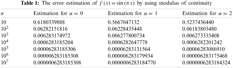
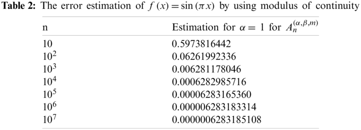
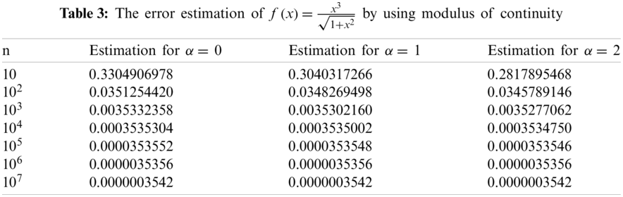
5  Numerical Example for An(α,β,m)

In this section we give some examples to obtain an upper bound for the error f(x)−An(α,β,m)(f;x) in the terms of the modulus of continuity. The computations in this paper were performed by using Maple2021TM.

Example 5.1. Let β = 1, m = η = 0, and n = 0,…,7. The approximation of An(α,β,m) to f = sin(π x) depends on α parameter on [0,∞) is shown in the Table 1.

Example 5.2. Let β = 1, m = η = 1 and n = 0,…,7. The approximation of An(α,β,m) to f = sin(π x) depends on α parameter on [0, ∞) is shown in the Table 2.

Example 5.3. The approximation of An(α,β,m) to f(x)=x31+x2 on [0, ∞) for fixed β = 1, m = η = 0, and n = 0,…7, is shown in the Table 3.

6  Conclusion

In the present paper, we have introduced a form of the operator using the generating function of Apostol-Genocchi polynomials of order α and obtained the approximation properties and rate of convergence of this operator. At the end of the paper, we have found an upper bound for the error f(x)−An(α,β,m)(f;x) in the terms of the modulus of continuity for some functions. For further works, the approximation properties studied for Szász type operators involving Apostol-Genocchi polynomials can also work for Kantorovich–Szász type operators involving Apostol-Genocchi polynomials, moreover, the q analogues of various modifications of Apostol–Genocchi polynomials of order α can discuss.

Acknowledgement: The author would like to thank the editor and referees for their many valuable comments and suggestions to improve the overall presentation of paper.

Funding Statement: The author received no specific funding for this study.

Conflicts of Interest: The author declares that he has no conflicts of interest to report regarding the present study.

References

 1.  Weierstrass, K. (1885). Über die analytische Darstellbarkeit sogenannter willkürlicher Functionen einer reellen Veränderlichen. Sitzungsberichte der Akademie zu Berlin, 2, 633–639. [Google Scholar]

 2.  Bernstein, S. (1912). Démonstration du théorème de Weierstrass fondée sur le calcul des probabilités. Communications of the Kharkov Mathematical Society, 13, 1–2. [Google Scholar]

 3.  Baskakov, V. A. (1957). An example of a sequence of linear positive operators in the space of continuous functions. Doklady Akademii Nauk SSSR, 113(2), 249–251. [Google Scholar]

 4.  Cheney, E. W., Sharma, A. (1964). Bernstein power series. Canadian Journal of Mathematics, 16, 241–252. DOI 10.4153/CJM-1964-023-1. [Google Scholar] [CrossRef]

 5.  Meyer-König, W., Zeller, K. (1960). Bernsteinsche potenzreihen. Studia Mathematica, 19(1), 89–94. DOI 10.4064/sm-19-1-89-94. [Google Scholar] [CrossRef]

 6.  Pethe, S. (1983). On linear positive operators. Journal of the London Mathematical Society, 2(27), 55–62. DOI 10.1112/jlms/s2-27.1.55. [Google Scholar] [CrossRef]

 7.  Szász, O. (1950). Generalization of S. Bernstein’s polynomials to the infinite interval. Journal of Research of the National Bureau of Standards, 45(3), 239–245. DOI 10.6028/jres.045.024. [Google Scholar] [CrossRef]

 8.  Jakimovski, A., Leviatan, D. (1969). Generalized Szász operators for the approximation in the infinite interval. Mathematica (Cluj), 11(34), 97–103. [Google Scholar]

 9.  Ismail, M. E. H. (1974). On a generalization of Szász operators. Mathematica (Cluj), 16(39). [Google Scholar]

10. Ispir, N., Atakut, Ç. (2002). Approximation by modified Szász–Mirakjan operators on weighted spaces. Proceedings of the Indian Academy of Sciences: Mathematical Sciences, 112(4), 571–578. DOI 10.1007/BF02829690. [Google Scholar] [CrossRef]

11. Kajla, A., Agrawal, P. (2015). Approximation properties of Szász type operators based on Charlier polynomials. Turkish Journal of Mathematics, 39(6), 990–1003. DOI 10.3906/mat-1502-80. [Google Scholar] [CrossRef]

12. Mursaleen, M., Ansari, K. J. (2015). On Chlodowsky variant of Szász operators by Brenke type polynomials. Applied Mathematics and Computation, 271(5), 991–1003. DOI 10.1016/j.amc.2015.08.123. [Google Scholar] [CrossRef]

13. Sucu, S., Büyükyazc, I. (2012). Integral operators containing Sheffer polynomials. Bulletin of Mathematical Analysis and Applications, 4(4), 56–66. [Google Scholar]

14. Içöz, G., Varma, S., Sucu, S. (2016). Approximation by operators including generalized Appell polynomials. Filomat, 30(2), 429–440. DOI 10.2298/FIL1602429I. [Google Scholar] [CrossRef]

15. Atakut, Ç., Büyükyazc, I. (2016). Approximation by Kantorovich–Szász type operators based on Brenke type polynomials. Numerical Functional Analysis and Optimization, 37(12), 1488–1502. DOI 10.1080/01630563.2016.1216447. [Google Scholar] [CrossRef]

16. Tasdelen, F., Aktas, R., Altn, A. (2012). A Kantorovich type of Szász operators including Brenke-type polynomials. Abstract and Applied Analysis, 2012, 13. DOI 10.1155/2012/867203. [Google Scholar] [CrossRef]

17. Varma, S., Sucu, S., Içöz, G. (2012). Generalization of Szász operators involving Brenke type polynomials. Computers & Mathematics with Applications, 64(2), 121–127. DOI 10.1016/j.camwa.2012.01.025. [Google Scholar] [CrossRef]

18. Çekim, B., Aktas, R., Içöz, G. (2019). Kantorovich–Stancu type operators including Boas-Buck type polynomials. Hacettepe Journal of Mathematics and Statistics, 48(2), 460–471. DOI 10.15672/HJMS.2017.528. [Google Scholar] [CrossRef]

19. Usta, F. (2021). On approximation properties of a new construction of Baskakov operators. Advances in Difference Equations, 2021(269), 1–13. DOI 10.1186/s13662-021-03425-6. [Google Scholar] [CrossRef]

20. Luo, Q. M. (2009). Q-extensions for the Apostol–Genocchi polynomials. General Mathematics, 17(2), 113–125. [Google Scholar]

21. Araci, S., Khan, W. A., Acikgoz, M., Özel, C., Kumam, P. (2016). A new generalization of Apostol type Hermite–Genocchi polynomials and its applications. SpringerPlus, 5(860), 1. DOI 10.1186/s40064-016-2357-4. [Google Scholar] [CrossRef]

22. Srivastava, M. H., Masjed-Jamei, M., Reza Beyki, M. (2018). A Parametric Type of the Apostol–Bernoulli, Apostol–Euler and Apostol-Genocchi Polynomials. Applied Mathematics & Information Sciences, 12(5), 907–916. DOI 10.18576/amis/120502. [Google Scholar] [CrossRef]

23. Prakash, C., Verma, D. K., Deo, N. (2021). Approximation by a new sequence of operators involving Apostol-Genocchi polynomials. Mathematica Slovaca, 71 (in Press). [Google Scholar]

24. Deo, N., Kumar, S. (2020). Durrmeyer variant of Apostol–Genocchi–Baskakov operators. Quaestiones Mathematicae, 44(4), 1–18. DOI 10.2989/16073606.2020.1834000. [Google Scholar] [CrossRef]

25. Gadzhiev, A. D. (1976). Theorems of Korovkin type. Mathematical Notes of the Academy of Sciences of the USSR, 20, 995–998. DOI 10.1007/BF01146928. [Google Scholar] [CrossRef]

26. Devore, R. A., Lorentz, G. G. (2005). Constructive approximation. Berlin: Springer-Verlag. [Google Scholar]

27. Johnen, H. (1972). Inequalities connected with the moduli of smootness. Matematicki Vesnik, 9(24), 289–305. [Google Scholar]

28. Davis, P. J. (1976). Interpolation and approximation. New York: Dover. [Google Scholar]

This work is licensed under a Creative Commons Attribution 4.0 International License, which permits unrestricted use, distribution, and reproduction in any medium, provided the original work is properly cited.