Computer Modeling in Engineering & Sciences

DOI: 10.32604/cmes.2022.018000

ARTICLE

A Fast Small-Sample Modeling Method for Precision Inertial Systems Fault Prediction and Quantitative Anomaly Measurement

Hongqiao Wang1,* and Yanning Cai2

1Xi'an Research Institute of High-Tech, Xi'an, 710025, China
2Northwest University of Politics and Law, Xi'an, 710122, China
*Corresponding Author: Hongqiao Wang. Email: ep.hqwang@gmail.com
Received: 21 June 2021; Accepted: 29 July 2021

1  Introduction

As the emerging growth of demand for systems’ health monitoring and reliability estimation, the fault diagnosis and prediction problems have become a research focus at present [1–4]. To realize the full-process heath management of system, the data collection, real-time detection, state measurement, modeling, prediction and anomaly evaluation have become more and more important, especially for some precision devices and complex systems requiring high reliability [5,6]. Inertial system platforms are a kind of important precision devices used in many industrial fields, such as navigation, guidance and aerospace, which have the characteristics of difficult acquisition for state data and small sample scale, so the fault trend of the devices should be discovered as early as possible based on the limited data samples to prevent the occurrence of serious damages to the whole system. The fault state of system is actually an abnormal phenomena deviating from the normal state, so the early warning of fault may be realized by novelty recognition before the fault completely occurs [7–10]. The concrete method based on this idea is as follows: build the system's normal working state space directly using the system's normal features, and recognize the novel samples by detecting whether the deviation from the normal features is existed.

For system fault diagnosis and prediction problems using data-driven methods [11–14], one-class SVM (OCSVM) is a typical classification tool, which can identify the known object class(normal sample) and the unknown object class(novel sample). As a popular method, a lot of improved OCSVM algorithms are studied. For example, FernaNdez-Francos et al. [15] presented a υ-SVM based OCSVM. Amer et al. [16] proposed an enhanced OCSVM for unsupervised method of anomaly detecting. Yin et al. [17] and Xiao et al. [18] studied the robust OCSVM algorithms. Yan et al. [19] introduced the OCSVM algorithm to fault prediction in the online condition. Huang et al. [20] combined the wavelet T-F entropy and OCSVM, and applied the method to mechanical system fault prediction. In addition, the one-class classification and the learning algorithms are suitable for data-driven modeling of black-box problems, especially for some pattern recognition applications [21–23]. In the past few years, the OCSVM methods are also used for faults detection, identification and diagnosis [24,25]. To detect the novelty sample effectively, Yi et al. [26] presented a supervised novelty detection SVM, which is extended from OCSVM and has a fast learning speed. Miao et al. [27] presented a distributed model and its online learning method with OCSVM for anomaly finding. Moreover, although most of the OCSVMs are applied for the classification fields, Bhland et al. [28] extended the model to the regression modeling and automated design process. As another data-driven modeling method, the extreme learning machine model is also introduced to the prediction application field [29]. With the widespread utilization of deep learning, the idea of OCSVM is also applied in some deep neural networks. For example, by means of the combination of OCSVM and deep neural networks [30], the deep OCSVM algorithm is proposed [31,32], the one-class convolutional neural network and its applications are also studied [33]. Moreover, by introducing the idea of the adversarial learning, some one-class classification and the anomaly detection methods are proposed based the adversarial framework [34,35]. Considering the small sample scale and the online monitoring conditions of precision inertial devices fault prediction, the training samples’ scale for modeling is too small and the training speed is too fast for all of the deep neural network models. As a result, the deep learning methods are not the ideal solutions in this application situation.

The OCSVM model has good sparseness, namely, the specific form of the model is only decided by part of the samples in the training set, namely the support vectors (SVs). Even so, the modeling efficiency is still greatly decreased as the calculation of a large number of NSVs in the model optimization process. To enhance the modeling efficiency of the fault diagnosis and prediction applications, a synthetical method using SV pre-selection is proposed aiming at the precision inertial device fault prediction in the small sample condition, which realizes data-driven fault diagnosis, state prediction, anomaly detection and quantitative measurement. Considering an OCSVM model, the distribution characteristics of the support vectors in the high dimensional space from are analyzed, respectively. On this basis, a modeling method with the samples owning some geometry characters selected from the training set is also executed. The fault prediction efficiency can be greatly improved using the pre-selection of the non-support-vector samples in the condition of having no effect on the fault prediction capability of OCSVM.

In the remainder of this paper, the sections are organized as follows: in Section 2, the OCSVM method in fault prediction field and the supersphere models for OCSVM are introduced. The support vector pre-selection method for the supersphere model is studied detailedly in Section 3, the number calculation of pre-selected samples and the algorithm's complexity are also analysed. In Section 4, the fault prediction and quantitative anomaly measurement using SV pre-selection OCSVM is studied. Several experiments and result analysis are carried out in Section 5. Finally, we conclude in Section 6.

2  Supersphere Models for OCSVM

2.1 OCSVM Method in Fault Prediction Field

Suppose the system's state can be represented with a d-dimensional variable x={x1,x2…,xd}∈Rd. Let the sample set collected from the normal working state is D={xi}, i=1,2,…,l. With the generation of new sample x′, it is necessary to judge if the sample indicate the existence of the fault trend. The sample has the characteristic of non-output and unlabeled in the above mentioned problem. The key point of the problem lies in how to build the fault prediction model based on the sample set D. In this fault prediction condition, the samples representing the system normal working state are seemed as samples in the target class, and the target class samples commonly have the similar distribution in the feature space. Correspondingly, the samples representing the system anomaly working state belong to the non-target class, which have a scattering distribution, so the one-class target information can be regard as the main information source. Unlike the general supervised classification with two values, this classification method can be seemed as the semi-supervised classification. Through the above analysis, it can be concluded that the OCSVM model can be used for fault prediction problems.

In the research field of SVM, the OCSVM is first introduced from Schölkopf in 1999, which is originally applied to probability density estimation of functions. The main thought of the method is: suppose a dataset in the given input space Rn is given, and it satisfies a distribution with probability P. We hope to find a simple data sub-set S in the input space and approximate the distribution, subject to the probability, that the sample with the P distribution falling into the outside of S, satisfies a certain given probability v(0<v<1) . The OCSVM is an extension of the standard SVM, which has two realization approaches. We will introduce the main thought of the methods in the following subsections.

2.2 Supersphere Model of OCSVM

The form of training samples on the supersphere model of OCSVM is D={xi∈Rd|i=1,…,l}. To build the supersphere model, we firstly should map the samples to a new feature space with a nonlinear mapping function φ(⋅). Secondly, seeking for a minimum sphere with the center aand the radius Rin the new space, which can contain all the samples. For some sample points, some error may exist, we can introduce the ξi as the control variables. At the same time, the calculation of inner product in the new space could conveniently be substituted by the kernel functions satisfying the Mercer conditions. Namely, find a kernel function k(x1,x2) and let k(x1,x2)=φ(x1)⋅φ(x2), as a result, the optimization problem is

minR2+1vl∑i=1lξis.t.[φ(xi)−a][φ(xi)−a]T≤R2+ξiξi≥0,i=1,2,…,l(1)

In (1), v∈(0,1) plays a compromise role between the radius of the supersphere and the training samples’ number containing in the sphere. The slack factors can guarantee that more training samples are containing in the supersphere as far as possible under the condition of the supersphere is maximally compressed. To calculate the center a and the radius R, formula (1) can be transformed into its dual form (2), the deduce process is

min∑i,j=1lαiαjk(xi,xj)−∑i=1lαik(xi,xi)s.t.∑i=1lαi=10≤αi≤1v⋅l,i=1,2,…,l(2)

Solve the optimization problem (2), it can be found that most of the αi are 0, for the αi unequal to 0, the corresponding samples are still called support vectors, and the form of the supersphere is only decided by support vectors. We may analysis the relative location relationship of the sample between the high-dimensional space and the supersphere based on the different values of αi according to the following three situations:

If αi∈(0,1v⋅l), it means that xi satisfies [φ(xi)−a][φ(xi)−a]{\rm T}=R2, namely xi is a boundary sample, and locates at the surface of the supersphere as a support vector.

If αi=1v⋅l, it means that xi satisfies [φ(xi)−a][φ(xi)−a]{\rm T}>R2, namely xi is not a boundary sample, and locates outside of the supersphere as a non-support vector.

If αi=0, it means that xi satisfies [φ(xi)−a][φ(xi)−a]{\rm T}<R2, namely xi locates inside of the supersphere as a non-support vector.

Let ISV is a set of support vectors, and lSV is the support vectors’ number, the center of the obtained supersphere is a=∑i∈ISVαiφ(xi). According to the KKT condition, for the sample xi corresponding to 0<αi<1v⋅l, we can get

R2−[k(xi,xi)−2∑j∈ISVαjk(xj,xi)+c2]=0(3)

As a result, the radius R can be obtained. For a new sample z,

f(z)=[φ(z)−a][φ(z)−a]T−R2=k(z,z)−2∑i∈ISVαik(z,xi)+∑i∈ISV∑j∈ISVαiαjk(xi,xj)−R2(4)

If f(z)≤0, we can conclude that z is normal point, if not, z is a novel point.

3  Sample Set Optimization for the Supersphere Model

The OCSVM model is sparse, namely the decision form of the supersphere is only depend on the support vectors, so the algorithm's complexity may be reduced through simplifying the training set, which is similar to the two-class model of SVM. It also can be found that the probability distribution of the SVs in the high-dimensional mapping space has some characteristics, which provides possibility for the SV pre-selection. Now, we'll discuss how to realize the support vectors pre-selection from the training sample set, namely the sample set optimization, and how to improve the training efficiency of OCSVM.

Definition 1: Suppose a sample set D={xi∈Rd|i=1,2,…,l} is known, let the mapping form to the high-dimension feature space is φ(⋅), the central point of the feature space is m, so m has a form as

m=1l∑i=1lφ(xi)(5)

Definition 2: Suppose two sample points xandyare known, the vectors from the original point to the two sample points are respectively x→ and y→. Let the included angle of the two vectors in the high-dimensional space is θ(x→,y→), its form is

θ(x→,y→)=arccos⁡((φ(x)⋅φ(y))||φ(x)||||φ(y)||)(6)

Definition 3: Suppose two sample points x1 and x2 are known, let the distance of these two points is d(x1,x2), the form is

d(x1,x2)=||φ(x1)−φ(x2))||=k(x1,x1))−2k(x1,x2))+k(x2,x2)(7)

Definition 4: If the sample points x1 and x2 are mapping to the feature space with φ(⋅), the distance of the two points in the feature space satisfies Eq. (8), which implies the Eq. (7).

d2(x1,x2)=||φ(x1)−φ(x2)||2=φ(x1)⋅φ(x1)−2φ(x1)⋅φ(x2)+φ(x2)⋅φ(x2)=k(x1,x1)−2k(x1,x2)+k(x2,x2)(8)

3.1 Support Vector Pre-Selection Method for the Supersphere Model

Theorem 1: Suppose the training sample set is D={xi∈Rd|i=1,2,…,l}, according to the Eq. (2), the supersphere model can be constructed, and the optimal solution of the supersphere is α={α1,…,αl}. The samples with the non-zero Lagrange multipliers are selected from D, with which we can obtain new sets D~={xi|αi≠0, i=1, 2,…, l}, and α~={αi≠0|, i=1,2,…,l}. If the kernel function and model parameters are all the same, and suppose the optimal solution of the supersphere based on D~ is β~, it can be concluded that β~=α~.

Proof: Let the numbers of element in D~ and α~ are both lSV, ISV={i|αi≠0,i=1,…,l}, and the optimal solution is β~={β~i|i=ISV(1),…,ISV(lSV)}.

Set the optimization problem based on D is L1

minL1(α)=∑i,j=1lαiαjk(xi,xj)−∑i=1lαik(xi,xi)s.t.∑i=1lαi=10≤αi≤1v⋅l,i=1,2,…,l(9)

and the optimization problem based on D~ is L2

minL2(β~)=∑i,j∈ISVβ~iβ~jk(xi,xj)−∑i∈ISVβ~ik(xi,xi)s.t.∑i∈ISVβ~i=10≤β~i≤1v⋅l,i=ISV(1),…,ISV(lSV)(10)

If β~ is extended to β with the relationship βi={β~ii∈ISV0i∉ISV, i=1, …,l, it can be obviously find that ∑i∈ISVβ~i=1 and 0≤β~i≤1vl, so β is the feasible solution of L1. As α is the optimal solution of L1, it can be concluded that L1(α)≤L1(β), because

L1(β)=∑i,j=1lβiβjk(xi,xj)−∑i=1lβik(xi,xi)=∑i,j∈ISVβ~iβ~jk(xi,xj)−∑i∈ISVβ~ik(xi,xi)=L2(β~)(11)

L1(α)=∑i,j=1lαiαjk(xi,xj)−∑i=1lαik(xi,xi)=∑i,j∈ISVα~iα~jk(xi,xj)−∑i∈ISVα~ik(xi,xi)=L2(α~)(12)

In summary, L2(α~)≤L2(β~). It is obvious that α~ is the feasible solution of L2, and β~ is the optimal solution of L2, then we have L2(α~)≥L2(β~), as a result, L2(α~)=L2(β~). Considering the uniqueness of the optimal solution of L2, it can be concluded that β~=α~.

From Theorem 1, it can be concluded that the trained supersphere model won't be damaged if the NSVs are removed. The support vector pre-selection principle of the supersphere model is shown as Fig. 1. In the figure, there are five sample points x1∼x5. Based on the construction principle of supersphere, we can know that x1∼x3 are non-support-vectors, x4 and x5 are support vectors. Let the central point of the sample set is m, we can easily find that the sample points x4 and x5, which are far away from m, are more likely becoming the support vectors.

Figure 1: Support vector pre-selection principle of the supersphere model

Through the above analysis, we can conclude the supersphere model's support vector pre-selection algorithm as the following 3 steps:

   Step 1: For a given sample set D={xi∈Rd|i=1,2,…,l}, calculate the sphere center m=1l∑i=1lφ(xi) based on the Definition 1.

   Step 2: Considering Definition 3, the square of distance from the sample x to m in the high-dimensional space is

d2(x,m)=‖φ(x)−1l∑i=1lφ(xi)‖2=k(x,x)−2l∑j=1lk(x,xj)+1l2∑i=1l∑j=1lk(xi,xj)(13)

As 1l2∑i=1l∑j=1lk(xi,xj) is a constant, to reduce the calculation amount, only the former twoitems are considered.

   Step 3: For each sample point xi in D, calculate si according to

si=k(xi,xi)−2l∑j=1lk(xi,xj),(14)

and update the training set through the selection of the bigger si from D.

3.2 Number Calculation of Pre-Selected Samples

In the SV pre-selection process of the supersphere model, the number of pre-selected SVs is an important value to be calculated. Based on (8), it can be find that α={α1,…,αl} subjects to ∑i=1lαi = 1, 0≤αi≤1v⋅l, v∈(0,1). Considering the SVs, set αi>0, i=1,2,…,lsv, which means the SV number is lsv. With regard to the NSVs, set αj=0, j=lsv+1, lsv+2,…,l, as a result, it can be easily concluded as (15)

∑i=1lαi=∑i=1lsvαi+∑j=lsv+1lαi=1(15)

Then, from the relationship of values between αi and 1vl, it can be find that

1=∑i=1lsvαi≤lsv×1vllsv≥vl(16)

From the above-mentioned equations, we can conclude that the total SVs number of the supersphere OCSVM algorithm is vl at least, which also decides the number of pre-selected samples. About how to calculate and obtain the pre-selected samples, the process is: Firstly, rank the set of si(i=1,2,…,l) by the result of (14) using a descending order. Secondly, select vl corresponding samples from the training set based on the former vl elements in the rank set, and set the value with s′ for the vlth element. Thirdly, compare and calculate the value of difference between the latter element in the rank set and s′ successively. If the calculated value is m, the threshold is Θ, and they satisfy m<Θ, select the corresponding sample as a SV.

From the above-mentioned equations, we can conclude that the total SVs number of the supersphere OCSVM algorithm is vl at least, which also decides the number of pre-selected samples. About how to calculate and obtain the pre-selected samples, the process is: Firstly, rank the set of si(i=1,2,…,l) by the result of (14) using a descending order. Secondly, select vl corresponding samples from the training set based on the former vl elements in the rank set, and set the value with s′ for the vlth element. Thirdly, compare and calculate the value of difference between the latter element in the rank set and s′ successively. If the calculated value is m, the threshold is Θ, and they satisfy m<Θ, select the corresponding sample as a SV.

3.3 Complexity Analysis of Algorithm

The essence of the supersphere model construction is to solve the quadratic programming problem, the problem scale and the solving efficiency are related to the samples’ number in training set. The calculation complexity is the cubic of the summation of samples when the traditional quadratic programming is executed. The algorithm's space complexity is primarily decided by the storage of kernel function matrix. Let the sample number of the supersphere is l, we can find that the space complexity is O(l2) for the storage of kernel function matrix, and the time complexity for model optimization is O(l3). There are two steps in the supersphere algorithm based on the support vector pre-selection: 1) Pre-select l′ support vectors from the training set with l samples, this operation has a space complexity of O(2l), namely two vectors which can contain l items are required. One vector is used for the storage of the intermediate result on si,i=1,…,l in (8) and (14), the other one is used for storage of the values of si. The time complexity of this step is O(l2), which is from the sorting of si. 2) Execute the optimization problem on the base of support vector set and build a model. For kernel function matrix, the space complexity is O(l′2), and the complexity of time consumption for model optimization is O(l′3) in this step. As the set of support vectors usually is a fraction of the total training sample set, the pre-selection of SVs method for the supersphere model could reduce the space and time complexity.

4  Fault Prediction and Quantitative Anomaly Measurement Using SV Pre-Selection OCSVM

The OCSVM model based on SVs pre-selection has a faster modeling speed, which can improve the efficiency of fault prediction. For the samples with the form of feature vectors, the model can be applied directly. But for the time series, the phase space reconstruction is firstly needed, and then the fault prediction model with OCSVM could be built. The phase space reconstruction is a research method for system's dynamic behavior based on the limited measured data and the attractor reconstruction. In order to restore the phase space's geometrical structure of dynamic systems from the one-dimensional time series, the one-dimensional time series should be embedded into the m-dimensional space, which has the form as: suppose the observed time series from system is x(t), with t=1, 2,…,N. The dimension of the phase space is m, the fixed time delay is called the embedded delay τ, so the sample points in the space of phase are X(t)=(x(t),x(t−τ),x(t−2τ),…,x(t−(m−1)τ))T, with t=1,2,…,Np, Np=N−(m−1)τ. The time series can be used for novelty detection after the phase space reconstruction, which also provides the theoretical basis for the time series prediction using OCSVM. The main procedure on fault prediction using SVs pre-selection is:

1)    Suppose the collected sample series in the system's normal state is x(t), t=1,2,…,N. Execute the reconstruction of phase space for the time series, and the sample set can be obtained as D={xi∈Rd|i=1,…,N−(m−1)τ}.

2)    Pre-select the support vectors from D, and build the OCSVM model as the fault prediction model based on the selected sample set. For the supersphere model, calculate the variable's value range representing the relative location relationship between the samples in D and the supersphere according formula (10). Then the lower bounds of the two ranges are regarded as the respective threshold reference to judge whether the fault trend exist or not.

3)    Decide whether the time series value x(t′) at time t′ indicate the fault trend. The method is: firstly, construct the sample being adapt to the model as x(t′)=(x(t′),x(t′−τ),x(t′−2τ), ⋯,x(t′−(m−1)τ))T based on x(t′). Then x(t′) is substitute to the OCSVM model after the support vector pre-selection, and the variable value representing the relative location relationship between x(t′) and the supersphere can be calculated. Finally, the variable value is used for judging whether the fault trend exist through the comparison to the fault threshold.

To quantitatively measure the anomaly level of one sample, the anomaly indexes (AIs) [6] can be defined as follows.

Set a system's normal state ω1 can be described by a given sample set {vi,i=1,…,l}, if the sample set is known, it means the normal state ω1 of the system is also known, but the samples in the system's anomaly state or in system's fault state are both unknown. Then set p(vi|ω1) as the probability density of vi, and let ρ1=min(p(vi|ω1)), ρ2=max(p(vi|ω1)), ρ=p(v′|ω1), where v′ is a new sample. As a result, the anomaly level of sample v′can be quantitatively measured by the anomaly indexes AIs(v′) , which has a form as (17)

AIs(v′)={ 0 ρ≥ρ20.5ρ−ρ2ρ1−ρ2 ρ2+(ρ1−ρ2)/0.5<ρ<ρ21 ρ≤ρ2+(ρ1−ρ2)/0.5(17)

For the samples in ω1, it can be found that 0≤AI(vi)≤0.5, i=1,…,l. On this basis, suppose a threshold θ(0≤θ≤1) is selected, if AI(v′)≤θ, it means the new sample v′ having not fault trend; if AI(v′)>θ, it means the new sample v′ has a fault trend. In other words, if AIs satisfies the condition AI(v′)≤θ, the sample v′ can be regarded as a normal sample; and if AI satisfies the condition AI(v′)>θ, it implies that the new sample v′ has a fault trend.

5  Experiments and Result Analysis

5.1 A Simulation Experiment and Analysis of Result

For the supersphere model, the training set is constructed from θ∈U[0,2π], ρ∈U[6,10], and 1000 samples are random generated, so the coordinates of θ and ρ are dimensionless. The RBF kernel is chosen and the pre-selected SVs are shown in Fig. 2.

Figure 2: Support vector pre-selection result of the supersphere model

Considering Fig. 2, it can be concluded that the obtained samples’ set through SV pre-selection of the supersphere model covers most of the SVs. As the supersphere model's training process is entirely unrelated to NSVs, it's obvious that the SV pre-selection approach may enhance the training efficiency in the condition of guaranteeing the model's novelty detection capacity.

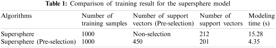
The supersphere algorithm's training results of the simulation samples are shown in Table 1. From data in the table, we also can find the speed of modeling is tremendously enhanced; as a result, the fault prediction and the anomaly measurement efficiency can also be enhanced.

5.2 Experiments for the Single-Dimensional Drift Data of Gyroscope

When the gyroscope devices are working in the normal state, their drift coefficients satisfy a certain transformation rule. When the fault trend exists, the original transformation rule will inevitably occur the drift, even exceed the normal working range. If we find the drift of transformation rule by the fault prediction model, or the working parameters will soon deviate from the normal working range, the fault trend must be predicted. If we find the transformation rule keeps the original state, and locates in the normal range, the conclusion having no fault trend should be given.

In this experiment, the samples come from the reliability experiments of the new gyroscopes. The experiment parameters include the gravitational acceleration g and the geographical latitude R, where g=979.4121cm/s−2, R=34.6006∘.

A data gathering system with special sensor is used for data acquisition and drift data storage. Based on the 91 groups of testing data in the dataset, the supersphere model is trained to detect whether the fault trend exists. Set the dimension of the unlabeled samples is 3, and construct 89 samples, the former 75 samples are used for modeling, and the latter 15 samples are used for fault prediction.

To evaluate the reliability of the experimental results, the experiment with the supersphere model of OCSVM is executed, and the modeling result is described in Fig. 3, which is the support vector pre-selection result. In Fig. 3a, the horizontal ordinates are the sample series numbers, and the vertical ordinate are the corresponding values of Lagrange multipliers, the values decide whether the samples are support vectors. Fig. 3b shows the location relationship between the samples and the supersphere, which is a unitless value of distance. As the pre-selected sample set includes all the SVs of the supersphere model, the results have the same form for the supersphere and the supersphere(SV pre-selection).

Figure 3: Modelling result of supersphere. (a) Support vector pre-selection (b) Location relationship between the samples and the supersphere

Utilizing the modeling result, the density distribution of the variable representing the relative location of the samples and the supersphere can be estimated as Fig. 4a. On this basis, the sample's anomaly indexes (AIs) are calculated. As shown in Fig. 4b, we still can see that the AIs are all below 0.5, namely there is not any fault trend exists in the gyroscope.

Figure 4: Result of anomaly indexes. (a) Density estimation (b) Calculation of AIs

5.3 Experiments for a Precision Inertia System Platform

The inertia system includes three gyroscopes, and we can get 8 drift ampere values of the precision platform by testers, which are the IY−up, IY−down, IX−up, IZX−up, IX−down, IZX−down, IZ−up, IZ - down. Based on the 8 values, 6 drift coefficients of the three gyroscopes can be deduced, the methods are: KOY=12(IY−up + IY−down)⋅KcY, KOX=12(IX−up+IX−down)⋅KcX, KOZ=12(IZ−up+IZ−down)⋅KcZ, KSY=−12(|IY−up| + |IY−down|)⋅KcY+Ωsin⁡φ, KSX=−12(|IX−up| + |IX−down|)⋅KcX+Ωsin⁡φ, KIZ=12(IZX−up + IZX−down)⋅KcZ, where φ is the geographical latitude of testing point, KcX, KcY, KcZ, Ω are constants if the testing target is known.

The sample form of the precision platform is X={KOY,KOX,KOZ,KSY,KSX,KIZ}. There are 130 groups of data with the 6-dimensional drift coefficient gathering from 2001 to 2007, as shown in Fig. 5. The values in this figure are all practical values of the precision platform's drift coefficients. The horizontal ordinates are the sample series numbers, and the vertical ordinate are the practically measured data.

The goal of the experiment is to analysis the platform's working state in 2007 based on the data from 2001 to 2006. There are 74 samples matching the system performance requirement in the six years, and these data are considered as the training samples to build the supersphere model with OCSVM. Fig. 6a is the support vector pre-selection result. In this subfigure, the horizontal ordinates are the sample series numbers of the drift time series, and the vertical ordinates are the values of Lagrange multipliers, the selected support vectors are used to build the supersphere model. The variable values representing the relative location of the samples and the supersphere are then calculated, as shown in Fig. 6b. In this subfigure, the horizontal ordinates are the whole samples including the training and the testing samples, and the vertical ordinates are the relative distances between the samples and the supersphere. If the relative distance is negative, it means the sample is inside the supersphere; if the distance is 0, it means the sample is on the supersphere surface; and if the distance is larger than 0, it means the sample is outside the supersphere.

Figure 5: Practical values of the precision platform's drift coefficients

Utilizing the modeling result, we can calculate the sample's anomaly indexes (AIs) by probability density estimation method, as shown in Fig. 7. It can be found that the AIs of the anomaly samples are all below 0.5 among the 118 samples from 2001 to 2006, which means the AIs can distinguish the normal samples and the anomaly samples. Considering the 4th sample in the 12 samples from 2007, namely the 122th sample in Fig. 7, the AI value is 0.5268, the AIs of the remaining 8 samples are all below 0.5. By analyzing the drift data of the platform's normal state from 2001 to 2006, we can obtain the practical drift range is [−0.5423, 0.5508]. it means that although the 122th sample's AI value is bigger than 0.5, namely the platform is beyond the normal working range in the past, but it still didn't exceed the drift range of the engineering permission. So, we can conclude that the precision platform had no obvious drift fault trend and had a stable running state in 2007.

Figure 6: Modelling result of supersphere. (a) Support vector pre-selection (b) Location relationship between the samples and the supersphere

Figure 7: Result of anomaly indexes (AI)

6  Conclusions

In this paper, a fast small-sample supersphere one-class SVM modeling method using SVs pre-selection is systematically studied, aiming at the data-driven fault state prediction and quantitative degree measurements. (1) The essence of the method lies in two aspects. firstly, construct the supersphere space model based on the samples from the system's normal state; secondly, compare the relative location relationship between the new sample and the supersphere to judge whether the sample deviates from the system's normal state. As a result, the fault prediction goal is reached. (2) The advantages of the method lie in the easily acquisition of data samples, the fast modeling and the strong sensibility to the system's anomaly. (3) The disadvantage is that it cannot track the fault trend continually, so there is a lack of further understanding for the fault trend. (4) When the system's fault trend occurs, how to build the efficient prediction model is the key problem to be solved. The OCSVM fault prediction model is mainly studied based on SV pre-selection. To improve the modeling efficiency, the SV pre-selection method for the supersphere model is proposed. The methods can extract the outside points and boundary points of the supersphere, and can give good fault prediction capability and effectiveness of quantitative anomaly measurement for precision inertial devices. The experiments on precision inertial systems testify that the proposed method has good fault prediction speed and precision, and can effectively quantitative measure the anomaly level of systems.

Acknowledgement: We thank the editors for their rigorous and efficient work, and we also thank the referees for their helpful comments.

Funding Statement: This work was jointly supported by the National Natural Science Foundation of China (Grant No. 61403397) and the Natural Science Basic Research Plan in Shaanxi Province of China (Grant Nos. 2020JM-358, 2015JM6313).

Conflicts of Interest: The authors declare that they have no conflicts of interest to report regarding the present study.

This work is licensed under a Creative Commons Attribution 4.0 International License, which permits unrestricted use, distribution, and reproduction in any medium, provided the original work is properly cited.