| Computer Modeling in Engineering & Sciences |
DOI: 10.32604/cmes.2022.017355
ARTICLE
Hybridization of Differential Evolution and Adaptive-Network-Based Fuzzy Inference System in Estimation of Compression Coefficient of Plastic Clay Soil
1University of Transport and Communications, Hanoi, 100000, Vietnam
2Department of Civil, Environmental and Natural Resources Engineering, Lulea University of Technology, Lulea, 971 87, Sweden
3Department of Watershed & Arid Zone Management, Gorgan University of Agricultural Sciences & Natural Resources, Gorgan, 4918943464, Iran
4University of Transport Technology, Hanoi, 100000, Vietnam
5DDG (R) Geological Survey of India, Gandhinagar, 382010, India
*Corresponding Authors: Nadhir Al-Ansari. Email: nadhir.alansari@ltu.se; Binh Thai Pham. Email: binhpt@utt.edu.vn
Received: 04 May 2021; Accepted: 12 July 2021
Abstract: One of the important geotechnical parameters required for designing of the civil engineering structure is the compressibility of the soil. In this study, the main purpose is to develop a novel hybrid Machine Learning (ML) model (ANFIS-DE), which used Differential Evolution (DE) algorithm to optimize the predictive capability of Adaptive-Network-based Fuzzy Inference System (ANFIS), for estimating soil Compression coefficient (Cc) from other geotechnical parameters namely Water Content, Void Ratio, Specific Gravity, Liquid Limit, Plastic Limit, Clay content and Depth of Soil Samples. Validation of the predictive capability of the novel model was carried out using statistical indices: Root Mean Square Error (RMSE), Mean Absolute Error (MAE), and Correlation Coefficient (R). In addition, two popular ML models namely Reduced Error Pruning Trees (REPTree) and Decision Stump (Dstump) were used for comparison. Results showed that the performance of the novel model ANFIS-DE is the best (R = 0.825, MAE = 0.064 and RMSE = 0.094) in comparison to other models such as REPTree (R = 0.7802, MAE = 0.068 and RMSE = 0.0988) and Dstump (R = 0.7325, MAE = 0.0785 and RMSE = 0.1036). Therefore, the ANFIS-DE model can be used as a promising tool for the correct and quick estimation of the soil Cc, which can be employed in the design and construction of civil engineering structures.
Keywords: Compression coefficient; differential evolution; adaptive-network-based fuzzy inference system; machine learning; vietnam
Soil is a natural resource formed due to weathering of different rocks, comprising of various minerals, air, water, and organic material. The determination of the geotechnical properties of soil is very important for the safe and economic construction of civil engineering structures [1–4]. Soil properties, especially compressibility or compression coefficient (Cc) depend on the types of soils and it’s in filled spaces [1]. Fine-grained soils have a relatively lower load tolerance capacity than coarse-grained soils [2]. Compressibility of soil which includes compaction and consolidation also affects agriculture and plant growth [5]. The conventional methods and tests for determining soil compaction parameters [6–8] and consolidation are costly and time-consuming process and require a great deal of precision [9]. Therefore, various theoretical and experimental models have been developed to establish the correlation between Cc and other soil index properties using minimum data [10].
Recently, Artificial Intelligence (AI) or Machine Learning (ML) techniques have been used to estimate engineering parameters and in solving geotechnical problems including compressibility, soil classification, and shear strength of soil [11–16]. Single algorithms such as Support Vector Machine (SVM), Artificial Neural Network (ANN) have been used successfully in geotechnical engineering. The quality of the input data is also essential for improving the performance of AI or ML models [17]. The application of ML and AI in predicting Cc, has been attempted by some researchers using ANN with seven input variables including water content, liquid limit, plastic index, specific gravity, and soil types, which revealed that the ANN model could perform better than empirical formulas [18]. In another study using the ANN model in estimating Cc of fine-grain soils, they found that the estimated values were obtained nearly equal to the experimental values [19]. Some studies indicated that Adaptive Neuro-Fuzzy Inference System (ANFIS) and Genetic expression programming performed better than existing empirical equations [20].
Recently, hybrid models using a combination of ML algorithms such as ANN, ANFIS, SVM, Multi-Layer Perceptron Neural Network (MLPNN), and Particle swarm optimization (PSO) have been efficiently used to predict soil parameters such as Cc [21,22]. Bui et al. [22] indicated that the hybrid model of Particle Swarm Optimization based Multi-Layer Perceptron (PSO-MLP) has the most accurate prediction of Cc in comparison with the single models of SVM, random forest, and Gaussian process, backpropagation neural network, and radial basis function. Another comparative study between hybrid models and single models also found that a hybrid model of ABC-LM-ANN (Artificial Bee Colony-Levenberg–Marquardt-Artificial Neural Network) could give a better performance compared to other benchmark approaches in predicting Cc for a housing construction project [23]. Moayedi et al. [24] also confirmed that a hybrid model of League Championship optimization Algorithm (LCA) and ANFIS outperformed the single model of ANFIS. Thus, they have concluded that the hybrid model of LCA-ANFIS could be a promising alternative to empirical methods.
Based on the above literature review on the application of ML and AI in predicting Cc, it can be accepted that both single and hybrid models could predict Cc with high accuracy, but in general, the hybrid models performed better than the single models. However, the application of hybrid models in estimating Cc still remains limited, thus it has been attempted in this study. In addition, model development and improvement are a continuous process. As a result, it is necessary to fill this gap in the literature by developing new hybrid models. Therefore, in this work, the main objective is to develop and use first time hybrid ML model namely: ANFIS-DE which is a combination of Differential Evolution (DE), which is one of the most popular optimization techniques, and ANFIS for better prediction or estimation of the soil Cc. For this, a dataset of 817 soil testing samples was used for the model study. The seven soil parameters which are easily determined in the laboratory such as: Water Content, Void Ratio, Specific Gravity, Liquid Limit, Plastic Limit, Clay Content, and Depth (of Soil Samples) were used as input variables for the estimation or prediction as output (Cc). These parameters of soil obtained from the construction projects in Red River Delta, Viet Nam, were used in the present study. Performance of the models was evaluated using statistical indices namely Mean Absolute Error (MAE), Root Mean Square Error (RMSE), and Correlation Coefficient (R). In addition, REPTree (Reduced Error Pruning Trees) and DStump (Decision Stump), which are popular ML models, were used for the comparison.
Methodology of this study is presented in Fig. 1, which includes several main steps such as: (i) The data of Cc and relevant soil parameters (factors) obtained from test results were randomly split into two parts: training (70%) and testing (30%) datasets, (ii) Training dataset was then used to construct the hybrid model ANFIS-DE; out of these, DE was used as an optimization technique which used to optimize the weights and bias of the ANFIS predictor through optimization of the main control parameters of ANFIS (γ and σ2), and (iii) The final step was carried out by validating the constructed ANFIS-DE by using a testing dataset and several common statistical indicators such as R, RMSE, MAE.

Figure 1: Methodological flowchart of this study
Detail description of the data used and methods applied is presented in the following sections.
In this study, the soil data of several construction projects located in Red River Delta, Viet Nam namely Thinh Long Bridge (32 samples), Nam Binh Bridge (31 samples), Bach Dang Bridge (34 samples), Ha Noi–Hai Phong National Highway (346 samples), Nam Dinh Coastal Roads (240 samples), Red River Bridge (28 samples), Tra Ly Bridge (25 samples), Van Giang Commercial Complex of Hung Yen province (36 samples), Thang Long Cement Factory of Quang Ninh province (45 samples) were used for the modeling. Red River Delta is formed by Red River (Hong River) and its distributaries in Northern Vietnam. This delta runs along the Gulf of Tonkin in 120 km length and extends 240 km in land. In total data of 817 soil samples (plastic clay) was used for the present study. The soil data was split in a 70:30 ratio randomly for the training (70%) and testing/validation (30%) of the models. In the modeling, geotechnical parameters namely depth of soil samples, clay content (%), water content (%), void ratio, specific gravity, liquid limit (%), and plastic limit (%) were used as input parameters and compressive coefficient (Cc) as output variable. Detail description of these parameters is presented in the following sections.
2.1.1 Compression Coefficient (Cc)
Compression coefficient (Cc) or compression index is an important soil mechanical parameter, which includes compaction and consolidation of soil [25]. It is an important factor in analyzing the settlement of foundation of structure in soft soil. The Cc is computed by the slope of the compression curve in the oedometer test (Fig. 2) [25]. In this study, the compression index of samples varies from 0.018 to 1.37 (Table 1). The data distribution of the compression coefficient parameter is presented in Fig. 3a.

Figure 2: Consolidation curve for over-consolidated clay [26]


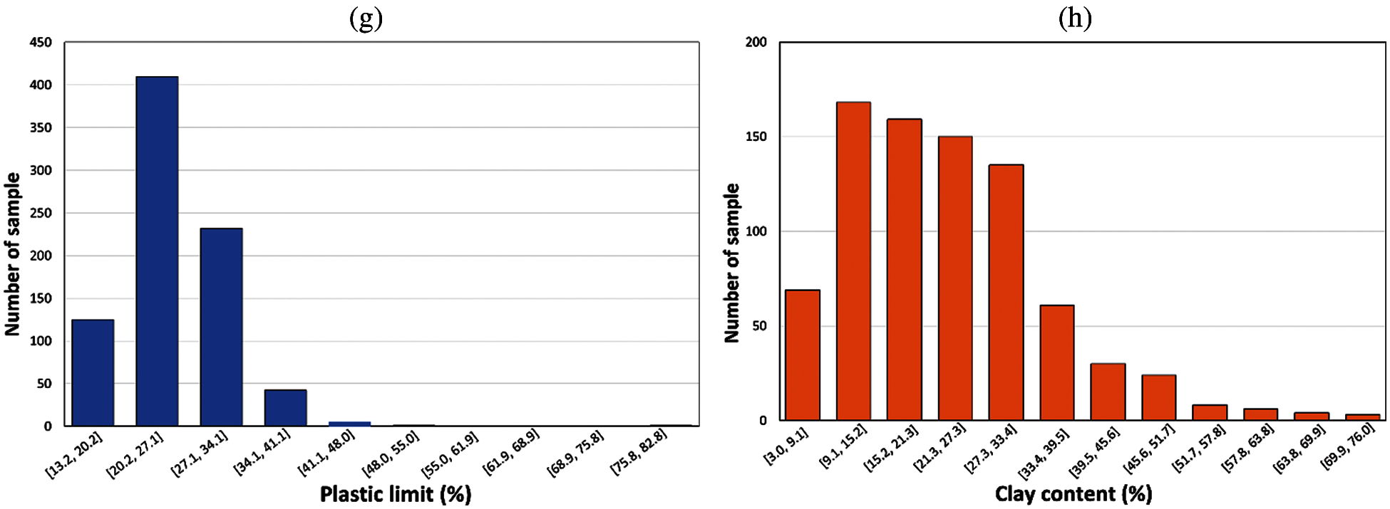
Figure 3: The data distribution plot of input parameters: (a) Compression coefficient; (b) Depth; (c) Water content; (d) Void ratio; (e) Specific gravity; (f) Liquid limit; (g) Plastic limit; and (h) Clay content
2.1.2 Depth of the Soil Samples
The depth at which soil samples were collected for the determination of engineering properties of soil is considered as one of the important factors in the assessment of consolidation of soil [25]. This is a critical input parameter in the prediction of the Cc. In the present work, samples from a depth varying between 1.1 and 45.85 m were collected and analyzed (Table 1). The data distribution of the depth parameter is presented in Fig. 3b.
Water content (w) is defined as the proportion of the specific volume of water to the weight of solids of soil [25]. It is one of the important variables in reducing cohesive forces between soil particles, shear strength of soils, and even causes the saturation of soils [27]. Consolidation of soils occurs when water is expelled from the pore spaces. Thus, it is a critical input parameter for the prediction of the Cc [28–30]. Water content can be calculated as following equation [31]:
where Ww is defined as the weight of water of soil sample, Ws is defined as the weight of solids of the soil sample, mw is defined as the mass of water of soil sample, ms is defined as the mass of the solids of the soil sample, and g is defined as the acceleration of gravity (g = 9.81 m/s2). In the present work, the water content of samples differs from 17.22% to 122.9% (Table 1). The data distribution of the water content parameter is presented in Fig. 3c.
“Void ratio (e) is defined as the ratio of the volume of voids to the volume of solids” [25]. It has a strong correlation with compression index [30,32–34]. It can be calculated as follows [25]:
where Vv is the volume of voids and Vs is the volume of soil solids. In the present work, the void ratio of samples differs from 0.508 to 3.31 (Table 1). The data distribution of the void ratio parameter is shown in Fig. 3d.
“Specific gravity (Gs) is defined as the ratio of the unit weight of a given material to the unit weight of water” [25]. It is an affecting factor to the compression index of soils [35]. The specific gravity of the soil is given by the following equation [36]:
where ρs is the particle density of soil and pw is the density of water (pw = 1000 kg/m3). In this study, the specific gravity of samples differs from 2.5 to 2.78 (Table 1). The data distribution of specific gravity parameter is shown in Fig. 3e.
“Liquid limit (LL) is defined as the moisture content at the point of transition from plastic liquid state”. It is strongly correlated with the compression index of soils [37,38]. The values of this factor can be determined by Atterberg tools in the laboratory, and using the following equation [25]:
where Ws is the weight of solids of the soil sample, Wliquid is defined as the weight of water of the soil sample at the point of transition from plastic to liquid state. In the present work, the liquid limit of samples differs from 20.7% to 127.9% (Table 1). The data distribution of the liquid limit parameter is presented in Fig. 3f.
Plastic Limit (PL) is the moisture content at the point of transition from semisolid to plastic state, which can be determined using Atterberg tools in the laboratory. It is a critical input factor in the prediction of the Cc, which is calculated using the following equation [25]:
where Wplastic is the weight of water of soil sample at the point of transition from semisolid to plastic state. In the present work, the plastic limit of samples differs from 13.22% to 82.8% (Table 1). The data distribution of the plastic limit parameter is shown in Fig. 3g.
Clays are classified as soil solid smaller than 0.002 mm or between 0.002 and 0.005 mm in size [25]. Clay content (μ) is an influencing factor to the compression index of soils, which can be determined in the laboratory through grain size distribution analysis based on the following equation:
where msum is defined as the total mass of the soil sample and m0.005 is defined as the mass of soil passing through 0.005 mm sieve. In the present work, the clay content of samples ranges from 3% to 76% (Table 1). The data distribution of the clay content parameter is shown in Fig. 3h.
2.2.1 Adaptive-Network-Based Fuzzy Inference System (ANFIS)
Fuzzy set theory was proposed in 1965 to describe linguistic expressions as a mathematical method. An ANN is a practical method for learning various functions, such as functions with real values, functions with discrete values, and functions with vector values, which are based on the interconnection of several processing units [39]. The fuzzy-neural model is an extended fuzzy model that uses an ANN learning algorithm to teach the model. ANFIS is a hybrid fuzzy-neural network used to model complex systems. The most important reason for combining fuzzy systems with neural networks is their ability to learn [40]. The ANFIS model consists of a hybrid learning algorithm that includes a combination of the least-squares error algorithm and the reduction slope algorithm [41].
In this model, a set of nonlinear parameters is used in the hypothesis section and a set of linear parameters is used for the result section. Obtaining the value of these parameters is usually done in two steps forward and backward. In the first step, which goes to the fourth layer, the set of nonlinear parameters is assumed to be fixed and the set of linear parameters are calculated using the least-squares error algorithm. In the second step, the set of fixed linear parameters is assumed and the set of nonlinear parameters is obtained using the reduction slope algorithm [42]. The ANFIS output is calculated using the output parameters in the forward step. Output error is used to match the assumed parameters using the standard post-emission algorithm. It has been proved that the hybrid algorithm is very efficient in teaching the ANFIS model [43]. To determine the structure of the model, several methods have been proposed, the most common of which are the network separation method and reduced fuzzy clustering. The main difference between the two methods is in how to determine the fuzzy membership function. In the network separation method, the type and number of membership functions of the input information are determined by the input information [44].
2.2.2 Differential Evolution (DE)
All-purpose optimization evolution algorithms are known to be able to find near-optimal solutions to mathematical and real problems, while classical and analytical methods are not able to find the optimal solution in a logical computational time. One of these evolutionary algorithms that has recently been proposed is the “differential evolution algorithm” [45]. This algorithm uses a differential operator to generate new answers, which causes the exchange of information between samples. The most important features of the DE algorithm are its high speed, simplicity, and power. This method only starts with setting three parameters [46]. The population number parameter, the mutation weight parameter, and the C parameter are the probability of recombination or intersection, which is multiplied by the difference of the two vectors and added to the third vector. The F parameter is usually set between 0 and 2 and the Cr parameter is between 0 and 1 [47]. In general, this algorithm has different stages, mutation, intersection or recombination, and finally the selection, which is described in Fig. 4 [48].

Figure 4: Flowchart of DE optimization
2.2.3 Reduced Error Pruning Trees (REPTree)
REPTree algorithm is a type of speed decision algorithm. According to this algorithm, the information obtained and the error due to variance are reduced. In other words, the REPTree algorithm uses two methods in synthetic with Reduced Error Pruning “REP” and the Decision Tree “DT” [12]. The algorithm is generated using the information of two regression and decision trees for the classification standard. It is noteworthy that the difficulty and complexity of decision algorithms using pruning are reduced as well as the error due to model variance. This is why the simple structure of decision tree algorithms has led to consideration for classification purposes [49]. When the output of this process is high, the DT algorithm uses a series of training data to facilitate the modeling process and the REP to reduce the difficulty of the DT framework [50]. There is an overload overfitting-backward problem in the REPTree algorithm. After pruning the trees, the decision is to choose one of the best trees or one of the most accurate versions. The efficiency of this algorithm is according to notifications obtained from entropy or reduction of variance and reduction of error pruning methods [51]. In this study, the REPTree was trained with the optimal hyper-parameters such as: the bathsize is 100, the number of folds is 3, and the minimum total weights of the instances in a leaf are 2.
Dstump algorithm is a subset of machine learning algorithms [52]. This algorithm is is a type of DT model that includes an interior root or node that straight joint to the end nodes. It should be noted that DTs have an upward trend. It also uses three parameters as input variables. The first variable is the selection threshold “θ”, the second variable is a time period “tp” and the third variable is the sincerity/purity index [53]. Thus, a Dstump, statistical data continues until a limited period of time. The fi ∈ F property is then evaluated based on σ (⋅). On the other hand,
In this work, the statistical measures of “Root Mean Square Error (RMSE)”, “Mean Absolute Error (MAE)” and “Correlation Coefficient (R)” were used to validate and compare the models. Based on the RMSE and MAE indices, the smaller the difference between the actual and simulated data can be, the more reliable the simulation results [57]. Also, according to the RMSE and MAE indices, the closer the results of these are two indices are to zero, the more accurate and efficient the algorithms [58]. R is a statistical tool to determine the type and degree of relationship of one quantitative variable with another quantitative variable [59]. This coefficient is between 1 and −1 and if there is no relationship between the two variables, it is equal to zero [60]. These indicators are calculated based on the following formulas [61–64]:
where N is the total number of data, Xi is the ith simulated data, Yi is the ith observational data,
In this study, the ANFIS-DE was trained with the hyper-parameters such as: the number of populations is 50, lower bound of scaling factor is 0.2, upper bound of scaling factor is 0.8, and crossover probability is 0.5. Fig. 5 shows the optimization process of the ANFIS-DE with 1000 iterations. It can be observed that the R-value of the ANFIS-DE is dramatically increased in about 10 iterations and then stable with the value of approximate 0.8, while the values of RMSE and MAE are dramatically decreased in about 25 iterations and then stable with the values of 0.09 (RMSE) and 0.065 (MAE). These results show that the DE is dramatically optimized the predictive capability of the ANFIS, and thus, the performance of the ANFIS-DE is improved for the prediction of the Cc.

Figure 5: Optimization process of the ANFIS-DE model using different statistical indicators: (a) R, (b) RMSE, and (c) MAE
The correlation analysis results of actual (real) and predicted data of soil training and testing samples using the ANFIS-DE model showed that the R values for testing and training samples were 0.825 and 0.813, respectively (Fig. 6), which indicate that the predictive capability of the novel model ANFIS-DE is good for prediction of the Cc (Fig. 6).
Fig. 7 presents the results of the ANFIS-DE model error analysis using soil training samples. In this figure, it can be observed that the predicted value of the Cc obtained from the novel model is closer to the actual Cc value obtained from the experiment tests, which is also indicated by low values of RMSE (0.096) and MAE (0.065). This indicates that the novel model ANFIS-DE has a great goodness of fit with the training data. Fig. 8 shows the error analysis of the ANFIS-DE hybrid algorithm using soil testing samples. As can be seen, the predicted value of the Cc obtained from the novel model is closer to the actual Cc value obtained from the experiment tests, which is also indicated by low values of RMSE (0.094) and MAE (0.064). This shows that the predictive capability of the novel model ANFIS-DE is good for prediction of the soil Cc.

Figure 6: Correlation analysis of actual and predicted values of Cc using the ANFIS-DE model: (a) Training dataset and (b) Testing dataset

Figure 7: Error analysis of the ANFIS-DE model using the training dataset

Figure 8: Error analysis of the ANFIS-DE model using the testing dataset
3.2 Comparison of ANFIS-DE with Popular Single ML Models
Table 2 shows the comparison of single ML models (REPTree and DStump) and hybrid algorithm (ANFIS-DE) using R, RMSE, and MAE statistical indices for the training dataset, it can be seen that the accuracy of the ANFIS-DE algorithm based on R, RMSE, and MAE is 0.813, 0.096 and 0.065, respectively. Also, the accuracy of REPTree and DStump single algorithms is R = 0.8315 and 0.6699, RMSE = 0.0952 and 0.1272, MAE = 0.0683 and 0.0949, respectively. Therefore, it can be concluded that all three ML models had a great goodness of fit with the data used.

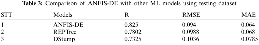
On the other hand, the comparison of hybrid and single ML algorithms using testing dataset showed that the statistical indices R, RMSE, and MAE in the ANFIS-DE hybrid algorithm are 0.825, 0.096, and 0.064, respectively (Table 3), and the efficiency of REPTree and DStump single algorithms in predicting and evaluating the Cc are (0.7802, 0.7325, and 0.0988) and (0.1036, 0.068, and 0.0785), respectively. Therefore, it can be stated that the hybrid model ANFIS-DE is better than other ML models (REPTree and Dstump) for the prediction of Cc. The result of this study is consistent with previous studies that the hybrid models performed better than the single models [22]. For example, Bui et al. [22] revealed that the hybrid model of PSO-MLP has the highest accuracy prediction of Cc in comparison with single models of SVM, Random Forest, and Gaussian process, etc. Besides, other authors also indicated that the hybrid model of LCA-ANFIS outperformed the single model of ANFIS [24].
In general, it can be stated that the novel hybrid model ANFIS-DE has the highest predictive capability compared with other single ML models (REPTree and Dstump). It might be due to the reason that in this hybrid model we have used ANFIS as a base predictor, which is able to model data with more capability. Also, by increasing the number of inputs in the ANFIS model to more than 4 inputs, different combinations of inputs are used in different ANFIS networks and finally enter the final ANFIS to support the output with very high accuracy [65]. In addition, the ANFIS model includes two models: neural networks and a fuzzy model. The fuzzy part establishes the relationship between input and output and the parameters related to the fuzzy part membership functions are determined by neural networks. Therefore, the characteristics of both fuzzy and neural models lie in ANFIS. For this reason, using the capabilities of both models can provide better results in hybrid model [66]. Since the hybrid algorithm has the features and characteristics of both algorithms and even the features of both individual exchange algorithms must be exchanged, generally, it has a very high accuracy and efficiency [67]. Also, the main positive features of hybrid models are high flexibility and reliability [68].
In the present study, soil compression coefficient (Cc) was estimated using a novel hybrid model namely ANFIS-DE, which is a combination of ANFIS and DE optimization techniques. REPTree and Dstump were also selected as benchmark ML models for the comparison. Soil parameters for the modeling were obtained from the analysis of 817 soil samples collected from various civil engineering projects located in Red Northern Delta area, Vietnam. Out of these, Water content, Void Ratio, Specific Gravity, Liquid Limit, Plastic Limit, Clay content, and Depth of Soil Samples were used as input variables and the Cc was used as output variable. Various statistical indicators namely R, RMSE, and MAE were used for the validation and comparison of the models.
The results show that the novel hybrid model ANFIS-DE has a good predictive capability for prediction of the soil Cc (R = 0.825, MAE = 0.064 and RMSE = 0.094), its performance is even better than other benchmark ML models namely REPTree (R = 0.7802, MAE = 0.068 and RMSE = 0.0988) and Dstump (R = 0.7325, MAE = 0.0785 and RMSE = 0.1036). Therefore, it can be concluded that the novel model ANFIS-DE is a promising tool for quick and accurate prediction of the soil Cc, which can be used in proper designing and safe construction of civil engineering structures.
As can be confirmed and verified by the experimental results, one important advantage of the hybrid ANFIS-DE is that it incorporated two powerful single methods (ANFIS and DE) to obtain a good prediction performance of Cc parameter. Thus, this hybrid model is able to provide a reliable prediction of this soil parameter to quickly support engineering decision-making. Finally, the proposed hybrid ANFIS-DE model is a new alternative model to fill the gap in the literature in the application of the hybrid model for estimating Cc and to assist geotechnical engineers in designing building foundation structures. Future studies could consider new robust optimization techniques to enhance the estimation performance of Cc. Besides, future direction of the present study may include applying this hybrid model of ANFIS and DE in the estimation of other parameters and in solving more civil engineering problems.
However, one limitation of this study is that the present hybrid model does not incorporate the feature selection method, thus adopting metaheuristic-based feature evaluation could be a potential direction of this study. Besides, in this study, we have used only ANFIS combined with DE for the development of hybrid model, it is desirable to explore more combination of other single models for the comparison and selection of best hybrid model. Finally, although this study was conducted with a large number of samples with seven input parameters, more numbers of variable input parameters may be considered in future studies using this hybrid model for further refining performance of the model.
Funding Statement: This research is funded by Ministry of Education and Training of Vietnam, Grant No. B2020-GHA-03, organized by the University of Transport and Communications, Hanoi, Vietnam.
Conflicts of Interest: The authors declare that they have no conflicts of interest to report regarding the present study.
1. Ten Damme, L., Stettler, M., Pinet, F., Vervaet, P., Keller, T. et al. (2019). The contribution of tyre evolution to the reduction of soil compaction risks. Soil and Tillage Research, 194, 104–283. [Google Scholar]
2. Stoessel, F., Sonderegger, T., Bayer, P., Hellweg, S. (2018). Assessing the environmental impacts of soil compaction in life cycle assessment. Science of the Total Environment, 630, 913–921. DOI 10.1016/j.scitotenv.2018.02.222. [Google Scholar] [CrossRef]
3. Nguyen, L. T., Nguyen, M. D., Nguyen, H. H. (2021). Analysis of impacting factors for soil-cement column combined high strength geogrid. Transport and Communications Science Journal, 72(1), 9–15. DOI 10.47869/tcsj.72.1.2. [Google Scholar] [CrossRef]
4. Nguyen, M. D., Nguyen, L. N. (2010). Geoenvironment with safety exploitation and use of urban underground. Transport and Communications Science Journal, 29, 65–69. [Google Scholar]
5. Keller, T., Sandin, M., Colombi, T., Horn, R., Or, D. (2019). Historical increase in agricultural machinery weights enhanced soil stress levels and adversely affected soil functioning. Soil and Tillage Research, 194(10), 104–293. DOI 10.1016/j.still.2019.104293. [Google Scholar] [CrossRef]
6. Carter, M., Bentley, S. P. (1991). Correlations of soil properties. London: Pentech Press Publishers. [Google Scholar]
7. Mohammadzadeh, S. D., Bolouri Bazaz, J., Vafaee Jani Yazd, S. H., Alavi, A. H. (2016). Deriving an intelligent model for soil compression index utilizing multi-gene genetic programming. Environmental Earth Sciences, 75(3), 262. DOI 10.1007/s12665-015-4889-2. [Google Scholar] [CrossRef]
8. Singh, A., Noor, S. (2012). Soil compression index prediction model for fine grained soils. International Journal of Innovations in Engineering and Technology, 1(4), 34–37. [Google Scholar]
9. Svalina, I., Galzina, V., Lujić, R., Šimunović, G. (2013). An adaptive network-based fuzzy inference system for the forecasting: The case of close price indices. Expert Systems with Applications, 40(15), 6055–6063. DOI 10.1016/j.eswa.2013.05.029. [Google Scholar] [CrossRef]
10. Hakami, B. A., Seif, E. S. S. A. (2019). Geotechnical aspects and associated problems of Al-Shuaiba Lagoon soil, Red Sea coast, Saudi Arabia. Environmental Earth Sciences, 78(5), 158. DOI 10.1007/s12665-019-8136-0. [Google Scholar] [CrossRef]
11. He, Q., Shahabi, H., Shirzadi, A., Li, S., Chen, W. et al. (2019). Landslide spatial modelling using novel bivariate statistical based naïve bayes, RBF classifier, and RBF network machine learning algorithms. Science of the Total Environment, 663(9), 1–15. DOI 10.1016/j.scitotenv.2019.01.329. [Google Scholar] [CrossRef]
12. Pham, B. T., Prakash, I., Singh, S. K., Shirzadi, A., Shahabi, H. et al. (2019). Landslide susceptibility modeling using reduced error pruning trees and different ensemble techniques: Hybrid machine learning approaches. CATENA, 175, 203–218. DOI 10.1016/j.catena.2018.12.018. [Google Scholar] [CrossRef]
13. Jaafari, A., Panahi, M., Pham, B. T., Shahabi, H., Bui, D. T. et al. (2019). Meta optimization of an adaptive neuro-fuzzy inference system with grey wolf optimizer and biogeography-based optimization algorithms for spatial prediction of landslide susceptibility. CATENA, 175(3), 430–445. DOI 10.1016/j.catena.2018.12.033. [Google Scholar] [CrossRef]
14. Chen, M. Y. (2013). A hybrid ANFIS model for business failure prediction utilizing particle swarm optimization and subtractive clustering. Information Sciences, 220(3), 180–195. DOI 10.1016/j.ins.2011.09.013. [Google Scholar] [CrossRef]
15. Ding, W., Nguyen, M. D., Salih Mohammed, A., Armaghani, D. J., Hasanipanah, M. et al. (2021). A new development of ANFIS-based Henry gas solubility optimization technique for prediction of soil shear strength. Transportation Geotechnics, 29(8), 100579. DOI 10.1016/j.trgeo.2021.100579. [Google Scholar] [CrossRef]
16. Lim, C. S., Mohamad, E. T., Motahari, M. R., Armaghani, D. J., Saad, R. (2020). Machine learning classifiers for modeling soil characteristics by geophysics investigations: A comparative study. Applied Sciences, 10(8). DOI 10.3390/app10175734. [Google Scholar] [CrossRef]
17. de Andrade Barbosa, M., de Sousa Ferraz, R. L., Coutinho, E. L. M., Coutinho Neto, A. M., da Silva, M. S. et al. (2019). Multivariate analysis and modeling of soil quality indicators in long-term management systems. Science of the Total Environment, 657(3), 457–465. DOI 10.1016/j.scitotenv.2018.11.441. [Google Scholar] [CrossRef]
18. Park, H. Il, Lee, S. R. (2011). Evaluation of the compression index of soils using an artificial neural network. Computers and Geotechnics, 38(4), 472–481. DOI 10.1016/j.compgeo.2011.02.011. [Google Scholar] [CrossRef]
19. Kurnaz, T. F., Dagdeviren, U., Yildiz, M., Ozkan, O. (2016). Prediction of compressibility parameters of the soils using artificial neural network. SpringerPlus, 5(1), 1–11. DOI 10.1186/s40064-016-3494-5. [Google Scholar] [CrossRef]
20. Demir, A. (2015). New computational models for better predictions of the soil-compression index. Acta Geotechnica Slovenica, 12, 59–69. [Google Scholar]
21. Pham, B. T., Nguyen, M. D., Dao, D. V., Prakash, I., Ly, H. B. et al. (2019). Development of artificial intelligence models for the prediction of compression coefficient of soil: An application of Monte Carlo sensitivity analysis. Science of the Total Environment, 679, 172–184. DOI 10.1016/j.scitotenv.2019.05.061. [Google Scholar] [CrossRef]
22. Tien Bui, D., Nhu, V. H., Hoang, N. D. (2018). Prediction of soil compression coefficient for urban housing project using novel integration machine learning approach of swarm intelligence and multi-layer perceptron neural network. Advanced Engineering Informatics, 38, 593–604. DOI 10.1016/j.aei.2018.09.005. [Google Scholar] [CrossRef]
23. Samui, P., Hoang, N. D., Nhu, V. H., Nguyen, M. L., Ngo, P. T. T. et al. (2020). A new approach of hybrid bee colony optimized neural computing to estimate the soil compression coefficient for a housing construction project. Applied Sciences, 9(22). DOI 10.3390/app9224912. [Google Scholar] [CrossRef]
24. Moayedi, H., Bui, D. T., Dounis, A., Thao, P., Ngo, T. (2020). A novel application of league championship optimization: Hybridizing fuzzy logic for soil compression coefficient analysis. Applied Sciences, 10(1), 67. DOI 10.3390/app10010067. [Google Scholar] [CrossRef]
25. Das, B. M., Sobhan, K. (2013). Principles of geotechnical engineering. Massachusetts, USA: Cengage Learning. [Google Scholar]
26. Das, B. M. (2015). Principles of foundation engineering. Massachusetts, USA: Cengage Learning. [Google Scholar]
27. Sharma, B., Bora, P. K. (2003). Plastic limit, liquid limit and undrained shear strength of soil-reappraisal. Journal of Geotechnical and Geoenvironmental Engineering, 129(8), 774–777. DOI 10.1061/(ASCE)1090-0241(2003)129:8(774). [Google Scholar] [CrossRef]
28. Koppula, S. D. (1981). Statistical estimation of compression index. Geotechnical Testing Journal, 4(2), 68–73. DOI 10.1520/GTJ10768J. [Google Scholar] [CrossRef]
29. Lo, Y., Lovell, C. W. (1982). Prediction of soil properties from simple indices. USA: Transportation Research Board. [Google Scholar]
30. Azzouz, A. S., Krizek, R. J., Corotis, R. B. (1976). Regression analysis of soil compressibility. Soils and Foundations, 16(2), 19–29. DOI 10.3208/sandf1972.16.2_19. [Google Scholar] [CrossRef]
31. Whitlow, R. (2001). Basic soil mechanics. USA: Transport and Road Research Laboratory. [Google Scholar]
32. Nishida, Y. (1956). A brief note on compression index of soil. Journal of the Soil Mechanics and Foundations Division, 82(3), 160. DOI 10.1061/JSFEAQ.0000015. [Google Scholar] [CrossRef]
33. Hough, B. K. (1957). Basic soils engineering. New York, USA: UC Berkeley Transportation Library. [Google Scholar]
34. Gunduz, Z., Arman, H. (2007). Possible relationships between compression and recompression indices of a low-plasticity clayey soil. Arabian Journal for Science and Engineering Section B: Engineering, 32(2B), 179–190. [Google Scholar]
35. Koumoto, T., Park, J. H. (1998). Compression index equation for undisturbed clays. Transactions of the Japanese Society of Irrigation, Drainage and Reclamation Engineering, 1998(194), 255–259. [Google Scholar]
36. Knappett, J., Craig, R. F. (2012). Craig's soil mechanics. New York, USA: Taylor & Francis Group. [Google Scholar]
37. Skempton, A., Jones, O. T. (1944). Notes on the compressibility of clays. Quarterly Journal of the Geological Society of London, 100(1–4), 119–135. DOI 10.1144/GSL.JGS.1944.100.01-04.08. [Google Scholar] [CrossRef]
38. Terzaghi, K., Peck, R. B., Mesri, G. (1996). Soil mechanics in engineering practice. New York, USA: Wiley. [Google Scholar]
39. Badiei, S., Kardan, M. R., Raisali, G., Rezaeian, P., Moslehi, A. (2019). Unfolding of fast neutron spectra by superheated drop detectors using adaptive network-based fuzzy inference system. Nuclear Instruments and Methods in Physics Research Section A: Accelerators, Spectrometers, Detectors and Associated Equipment, 944(2), 162–517. DOI 10.1016/j.nima.2019.162517. [Google Scholar] [CrossRef]
40. Tay, A., Lafont, F., Balmat, J. F. (2020). Forecasting pest risk level in roses greenhouse: Adaptive neuro-fuzzy inference system vs artificial neural networks. Information Processing in Agriculture (In Press). DOI 10.1016/j.inpa.2020.10.005. [Google Scholar] [CrossRef]
41. Long, S., Li, W., Yang, W., Sun, B., Yang, C. et al. (2020). pH prediction of a neutral leaching process using adaptive-network-based fuzzy inference system and reaction kinetics. IFAC–PapersOnLine, 53(2), 11901–11906. DOI 10.1016/j.ifacol.2020.12.708. [Google Scholar] [CrossRef]
42. Hosseinzadeh, A., Zhou, J. L., Altaee, A., Baziar, M., Li, X. (2020). Modeling water flux in osmotic membrane bioreactor by adaptive network-based fuzzy inference system and artificial neural network. Bioresource Technology, 310. DOI 10.1016/j.biortech.2020.123391. [Google Scholar] [CrossRef]
43. Chen, H. Y., Lee, C. H. (2019). Electricity consumption prediction for buildings using multiple adaptive network-based fuzzy inference system models and gray relational analysis. Energy Reports, 5(8), 1509–1524. DOI 10.1016/j.egyr.2019.10.009. [Google Scholar] [CrossRef]
44. Naghibi, S. A., Salehi, E., Khajavian, M., Vatanpour, V., Sillanpää, M. (2021). Multivariate data-based optimization of membrane adsorption process for wastewater treatment: Multi-layer perceptron adaptive neural network vs. adaptive neural fuzzy inference system. Chemosphere, 267, 129–268. DOI 10.1016/j.chemosphere.2020.129268. [Google Scholar] [CrossRef]
45. Yuan, Y., Wang, X., Meng, X., Zhang, Z., Cao, J. (2021). A strategy for helical coils multi-objective optimization using differential evolution algorithm based on entropy generation theory. International Journal of Thermal Sciences, 164. DOI 10.1016/j.ijthermalsci.2021.106867. [Google Scholar] [CrossRef]
46. Kaya, E., Korkmaz, S., Sahman, M. A., Cinar, A. C. (2021). DEBOHID: A differential evolution based oversampling approach for highly imbalanced datasets. Expert Systems with Applications, 169. DOI 10.1016/j.eswa.2020.114482. [Google Scholar] [CrossRef]
47. Qiu, L., Tian, X., Zhang, J., Gu, C., Sai, S. (2021). LIDDE: A differential evolution algorithm based on local-influence-descending search strategy for influence maximization in social networks. Journal of Network and Computer Applications, 178(6), 102973. DOI 10.1016/j.jnca.2020.102973. [Google Scholar] [CrossRef]
48. Li, W., Meng, X., Huang, Y. (2020). Fitness distance correlation and mixed search strategy for differential evolution. Neurocomputing (In Press). 458, 514–525. DOI 10.1016/j.neucom.2019.12.141. [Google Scholar] [CrossRef]
49. Chen, W., Hong, H., Li, S., Shahabi, H., Wang, Y. et al. (2019). Flood susceptibility modelling using novel hybrid approach of reduced-error pruning trees with bagging and random subspace ensembles. Journal of Hydrology, 575, 864–873. DOI 10.1016/j.jhydrol.2019.05.089. [Google Scholar] [CrossRef]
50. Cestonaro, T., de Vasconcelos Barros, R. T.,de Matos, A. T.,Azevedo Costa, M. (2021). Full scale composting of food waste and tree pruning: How large is the variation on the compost nutrients over time? Science of the Total Environment, 754. DOI 10.1016/j.scitotenv.2020.142078. [Google Scholar] [CrossRef]
51. Burcham, D. C., Autio, W. R., Modarres-Sadeghi, Y., Kane, B. (2021). After pruning, wind-induced bending moments and vibration decrease more on reduced than raised Senegal mahogany (Khaya senegalensis). Urban Forestry & Urban Greening, 61. DOI 10.1016/j.ufug.2021.127100. [Google Scholar] [CrossRef]
52. Kokilavani, S., Sankaralingam, S. K. N., Narmadha, A. S. (2020). Energy aware decision stump linear programming boosting node classification based data aggregation in WSN. Computer Communications, 155(92), 133–142. DOI 10.1016/j.comcom.2020.02.062. [Google Scholar] [CrossRef]
53. Jian, Z., Shirai, H., Takahashi, I., Kuroiwa, J., Odaka, T. et al. (2007). Masquerade detection by boosting decision stumps using UNIX commands. Computers & Security, 26(4), 311–318. DOI 10.1016/j.cose.2006.11.008. [Google Scholar] [CrossRef]
54. Barddal, J. P., Enembreck, F., Gomes, H. M., Bifet, A., Pfahringer, B. (2019). Boosting decision stumps for dynamic feature selection on data streams. Information Systems, 83(1–2), 13–29. DOI 10.1016/j.is.2019.02.003. [Google Scholar] [CrossRef]
55. Bogdanski, B. E. C., Cruickshank, M., Mario Di Lucca, C., Becker, E. (2018). Stumping out tree root disease-an economic analysis of controlling root disease, including its effects on carbon storage in Southern British Columbia. Forest Ecology and Management, 409(3), 129–147. DOI 10.1016/j.foreco.2017.11.012. [Google Scholar] [CrossRef]
56. Bereta, M. (2019). Regularization of boosted decision stumps using tabu search. Applied Soft Computing, 79, 424–438. DOI 10.1016/j.asoc.2019.04.003. [Google Scholar] [CrossRef]
57. Nguyen, M. D., Pham, B. T., Ho, L. S., Ly, H. B., Le, T. T. et al. (2020). Soft-computing techniques for prediction of soils consolidation coefficient. CATENA, 195, 104802. DOI 10.1016/j.catena.2020.104802. [Google Scholar] [CrossRef]
58. Chen, J., Li, A., Bao, C., Dai, Y., Liu, M. et al. (2021). A deep learning forecasting method for frost heave deformation of high-speed railway subgrade. Cold Regions Science and Technology, 185(3), 103265. DOI 10.1016/j.coldregions.2021.103265. [Google Scholar] [CrossRef]
59. Ly, H. B., Nguyen, T. A., Mai, H. V. T. (2021). Compressive strength prediction of recycled aggregate concrete by artificial neural network. Transport and Communications Science Journal, 72(3), 369–383. DOI 10.47869/tcsj.72.1.2. [Google Scholar] [CrossRef]
60. Eem, S., Choi, I. K., Cha, S. L., Kwag, S. (2021). Seismic response correlation coefficient for the structures, systems and components of the Korean nuclear power plant for seismic probabilistic safety assessment. Annals of Nuclear Energy, 150(3), 107759. DOI 10.1016/j.anucene.2020.107759. [Google Scholar] [CrossRef]
61. Liemohn, M. W., Shane, A. D., Azari, A. R., Petersen, A. K., Swiger, B. M. et al. (2021). RMSE is not enough: Guidelines to robust data-model comparisons for magnetospheric physics. Journal of Atmospheric and Solar-Terrestrial Physics, 218(A3), 105624. DOI 10.1016/j.jastp.2021.105624. [Google Scholar] [CrossRef]
62. Hao, X., Qiu, Y., Fan, Y., Li, T., Leng, D. et al. (2020). Applicability of temporal stability analysis in predicting field mean of soil moisture in multiple soil depths and different seasons in an irrigated vineyard. Journal of Hydrology, 588(4), 125059. DOI 10.1016/j.jhydrol.2020.125059. [Google Scholar] [CrossRef]
63. Edelmann, D., Móri, T. F., Székely, G. J. (2021). On relationships between the pearson and the distance correlation coefficients. Statistics & Probability Letters, 61. DOI 10.1016/j.spl.2020.108960. [Google Scholar] [CrossRef]
64. Zeng, W., Wang, F., Miao, L., You, F., Yao, F. (2020). Laser ultrasonic melanoma detection in human skin tissues via pearson correlation coefficient. Optik, 222(6), 165478. DOI 10.1016/j.ijleo.2020.165478. [Google Scholar] [CrossRef]
65. Karthika, B. S., Deka, P. C. (2015). Prediction of air temperature by hybridized model (Wavelet-ANFIS) using wavelet decomposed data. Aquatic Procedia, 4(7), 1155–1161. DOI 10.1016/j.aqpro.2015.02.147. [Google Scholar] [CrossRef]
66. Ghiasi, M. M., Mohammadi, A. H., Zendehboudi, S. (2021). Use of hybrid-ANFIS and ensemble methods to calculate minimum miscibility pressure of CO2-reservoir oil system in miscible flooding process. Journal of Molecular Liquids, 331. DOI 10.1016/j.molliq.2021.115369. [Google Scholar] [CrossRef]
67. Asadzadeh, M. Z., Raninger, P., Prevedel, P., Ecker, W., Mücke, M. (2021). Hybrid modeling of induction hardening processes. Applications in Engineering Science, 5(4), 100030. DOI 10.1016/j.apples.2020.100030. [Google Scholar] [CrossRef]
68. Zhou, T., Gani, R., Sundmacher, K. (2021). Hybrid data-driven and mechanistic modeling approaches for multiscale material and process design. Engineering (In Press). DOI 10.1016/j.eng.2020.12.022. [Google Scholar] [CrossRef]
 | This work is licensed under a Creative Commons Attribution 4.0 International License, which permits unrestricted use, distribution, and reproduction in any medium, provided the original work is properly cited. |