Computer Modeling in Engineering & Sciences

DOI: 10.32604/cmes.2022.018652

ARTICLE

Numerical Analysis of Ice Rubble with a Freeze-Bond Model in Dilated Polyhedral Discrete Element Method

Biyao Zhai, Lu Liu and Shunying Ji*

State Key Laboratory of Structural Analysis for Industrial Equipment, Dalian University of Technology, Dalian, 116023, China
*Corresponding Author: Shunying Ji. Email: jisy@dlut.edu.cn
Received: 08 August 2021; Accepted: 09 September 2021

1  Introduction

Ice rubble is very common in cold regions; it consists of broken ice formed by the deformation, aggregation, and stacking of the floating ice sheet under the driving force of wind, wave, and current. Ice rubble can be defined as an “ice ridge” in lakes, seas, and oceans and an “ice jam” in rivers [1]; it could pose as a potential threat to bridge piers, lighthouses, pipelines, offshore wind turbines, and navigation system [2–4]. As ice blocks pile up in a relatively static state in the cold air and supercooling water, the interstitial water between the blocks can freeze and form a solid ice crust [5,6], which can consolidate the loose ice blocks, resist their relative movement, and alter the global mechanical performance of the ice rubble. The evaluation of the mechanical properties of ice rubble, whether consolidated or not, is a crucial problem that has attracted considerable attention.

Since the beginning of the seventies some investigations have been conducted on ice rubble and the effects of freeze-bonding on ice rubble. Laboratory and in-situ tests are two mainstream approaches at an early stage. The initial tests performed in laboratories were direct shear box tests [7–9]. Subsequently, biaxial shear tests [10–13], triaxial shear tests [14,15] and punch-through tests [16–18] have been conducted. Based on laboratory tests, an elastic-perfectly plastic model based on the Mohr–Coulomb law was proposed to describe ice rubble behavior [19,20]. Furthermore, in-situ punch-through experiments can provide reliable information about the properties and failure of ice rubble under actual environmental conditions [21–24].

To simulate ice rubble, the finite element method (FEM) and discrete element method (DEM) have mainly been used over the years. In FEM, ice rubble is modeled as a continuum and a homogeneous material. FEM has been successfully used in the simulation of punching tests of ice rubble [23,25–27]. However, as ice rubble is modeled as a continuum, FEM cannot provide detailed granular properties of the rubble, and there is uncertainty in determining whether there are enough blocks to consider the rubble as a continuum [28]. The DEM was developed by Cundall et al. [29] and was introduced by Hopkins and Hibler into ice simulations [30–32]. In the DEM, large deformations and discontinuous properties of ice can be modeled using the movement of individual ice blocks within it [33]. In addition, owing to its good performance in modeling the continuous breakage of ice, DEM has wide applications in ice engineering, e.g., ice ridge property experiments [34,35], interaction of ice with ships [36–38], and offshore structures [39–42]. Furthermore, the coupled FEM-DEM or FDEM provides a new alternative for analyzing the breaking process, in which the FEM is used to calculate the deformation of individual particles, while DEM is used for modeling the contact and movement of the particles or fragments [43,44]. This method has been successful in replicating the freeze bonding between individual rubble blocks in ice ridges in a two-dimensional space [28]. However, the FEM calculation for each DEM particle requires additional computation, which limits its application in practical engineering.

In this study, a freeze-bond model based on the dilated polyhedral DEM was proposed, in which the initialization of the bonds between individual particles is emphasized. The model was validated through several fundamental examples and then applied to simulate the freeze-bond effect on ice rubble.

2  Freeze-Bond Model Based on Dilated Polyhedral DEM

For modeling ice rubble consisting of arbitrary shapes of ice blocks, a dilated polyhedral element was constructed based on the Minkowski sum theory. To describe the freeze bonding between ice blocks and random pores in ice rubble, a new bond model was developed, inherited from the “interface-based” bond model and applied to simulate the breaking process of void-free material [45,46].

2.1 Dilated Polyhedral Element

The dilated polyhedral element was constructed using an arbitrary polyhedron dilated by a sphere element based on the Minkowski sum theory, as shown in Fig. 1 and formulated as [47]

A⊕B={x→+y→|x→∈A, y→∈B}, (1)

where A represents a polyhedron and B represents a sphere. The Minkowski sum theory essentially indicates sweeping one geometric feature around the surface of another geometric feature; for a dilated polyhedron, the theory indicates sweeping a sphere over the surface of a polyhedron. Through dilatation, the conventional vertices and edges of the polyhedron are transformed into spherical and cylindrical surfaces of the dilated polyhedron, allowing the easy and efficient detection of the contact between two elements.

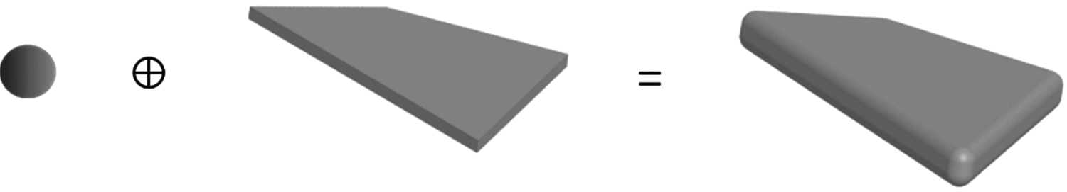
Figure 1: Dilated polyhedron constructed from a polyhedron and a sphere

Based on the theory on potential particles, the dilated polyhedron can be represented by approximate envelope function, which can be obtained by the weighted summation of the functions of polyhedron and sphere [48]. The second-order dilated function of the polyhedron can be expressed as:

f(x,y,z)=∑i=1N⟨aix+biy+ciz−di⟩2−r2, (2)

where (ai, bi, ci) is the unit normal vector of the face i on the polyhedron; N is the total number of faces in the polyhedron; ⟨⟩ is the Macaulay bracket, ⟨x⟩=x,x>0;⟨x⟩=0,x≤0; di is the distance of the coordinate origin to face i; r is the dilated radius. Accordingly, the approximate envelope function is given by:

f(x,y,z)=(1−k)(∑i=1N⟨aix+biy+ciz−di⟩2r2−1)+k(x2+y2+z2R2−1), (3)

where k is the weighting coefficient and R is the radius of the spherical function. The geometric shape represented by the function can approach the dilated polyhedron when k varies from 1 to 0.001. Therefore, it is assumed that the approximate envelope function can represent the dilated polyhedron when k reaches to 0.001.

In addition, the particle shape represented by the approximate envelope function belongs to “potential particle” so the contact detection for the contact center between two adjacent elements A and B can be solved by the optimization model between their respective functions. The corresponding non-linear equations based on the optimization algorithm can be expressed as:

{(1+λ)∇fA(X)+(1−λ)∇fB(X)=0fA(X)−fB(X)=0 (4)

where X = (x, y, z)T and λ is the Lagrange multiplier, fA and fB are the approximate envelope function of particles A and B, respectively. The Newton-Raphson method is used to solve the system of Eq. (4).

The initial point X0 is selected as the contact center between two minimum envelope spheres of each dilated polyhedron, which are expressed as:

X0=RBXOA+RAXOBRA+RB, (5)

where XOA and XOB are the mass center of each element, respectively; and RA and RB are the radii of the minimum envelope sphere of the elements. New initial points X0′ is obtained by Newton-Raphson iterations with the point X0, while the weighting coefficient k changes from 1 to 0.001. It can be used as the initial point in solving Eq. (4). For more details about the calculation of the overlap between dilated polyhedron elements, please refer to [48].

In the numerical simulation based on dilated polyhedron DEM, a given element has translational and rotational motions, which are calculated by the Newton’s second law of motion:

midvidt=∑j=1Nc(Fc)+∑j=1Nb(Fb)+Fe, (6)

Iidωidt=∑j=1Nc(Mc)+∑j=1Nb(Mb)+Me, (7)

where mi, Ii, vi, and ωi are the mass, inertia tensor, translation velocity, and angular velocity of element i, respectively; Fc, Fb, Mc, Mb are the contact force, bond force and their corresponding torques; Nc and Nb are the total number of particles in contact with element i and the total number of particles in bond with element i. Fe and Me are the forces and torques induced by external force.

2.2 Contact Model

Contact overlap and direction must be determined through DEM calculation. Liu et al. [48] proposed an approximate envelope function derived from the weighted summation of the second-order dilated function of polyhedral and spherical functions to represent dilated polyhedral. Thereby, the contact center can be determined using the optimization model between the approximate envelope functions of the two adjacent elements.

The Hertzian model, which exhibits good performance for nonspherical materials, was applied to calculate the contact force. Normal force Fn consists of normal elastic force Fne and viscous force Fnv, which are expressed as:

Fne=knδn32δ32, (8)

Fnv=−cn|δn|δ˙n, (9)

where kn is the normal contact stiffness, kn=4E∗r∗/3, E∗=E/2(1−ν2), r∗=rirj/(ri+rj), and ri and rj are the dilated radii; E and ν are the Young’s modulus and Poisson’s ratios, respectively; δn and δ˙n are the normal overlap and relative normal velocity, respectively; cn is the normal damping coefficient, cn=ζnmijkn and ζn=−ln⁡e/π2+ln2⁡e; e is the restitution coefficient; mij is the equivalent mass of two particles mi and mj; mij=mimj/(mi+mj).

The tangential contact force, Ft, includes elastic force Fte and viscous force Ftv, which are expressed as follows:

Fte=μ|Fne|[1−(1−δtδtmax)]t¯, (10)

Ftv=ct6μmij|Fne|1−δt/δtmaxδtmaxδ˙t, (11)

where μ and t¯ are the friction coefficient and unit direction vector, respectively; δt and δ˙t are the tangential relative displacement and velocity, respectively; δtmax is the maximum overlap in shear that characterizes the maximum tangential friction, δtmax=μδn(2−ν)/(2−2ν); ct is the damping coefficient in the tangential direction, ct=cn/2(1+ν).

2.3 Freeze-Bond Model

Because freeze bonding is generated at the contact positions between the ice blocks, a freeze bonding model was developed to connect the contact points of two particles that resist relative motion and rotation. As shown in Fig. 2, to sinter two particles, contact points P and P′ of two particles DP1 and DP2 are used to form a bond at the initialization step. Points Pc and Pc′ are the midpoints of P and P′, respectively, and are fixed on the local coordinates of particles DP1 and DP2, respectively. Subsequently, two imaginary bonding surfaces (face ABCD and face A′B′C′D′) are established at points Pc and Pc′, respectively, which are perpendicular to the line PP′. Points A,B,C, and D are four evenly distributed points centered at Pc on the bond face. Similarly, points A′,B′,C′, and D′ are centered at point Pc′. Points A,B,C,D, A′,B′,C′, and D′, called as bond points, are correspondingly coincident at the initial state and deform with the movement of their own particles. ni and nj are the outer normal vectors of each bond face and are initially in opposite directions.

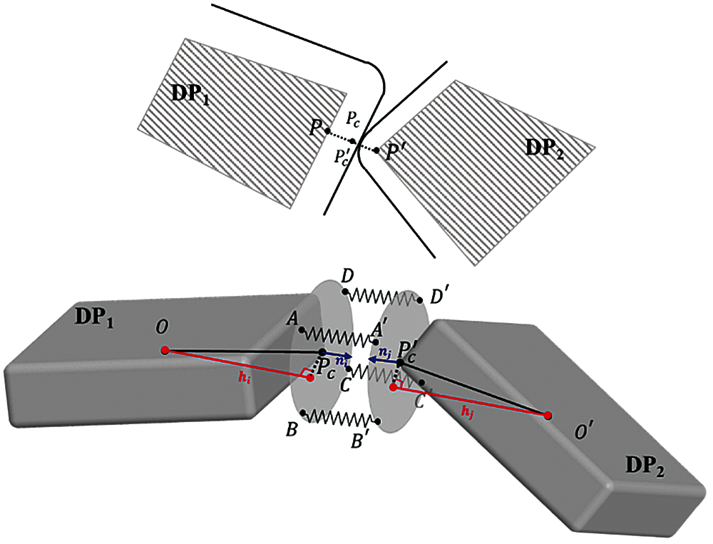
Figure 2: Bond model based on arbitrary contact

Cohesion between the two adjacent particles is established by the four sets of points, i.e., A–A′, B–B′, C–C′, and D–D′. The normal and shear forces are calculated based on the changes in their relative positions. Ultimately, the forces on the bond points are transferred to the mass centers (points O and O′) of the elements.

The normal strain can be obtained from the variation in the relative position of the bond point [46], which can be expressed as:

εnb=d⋅nLij, (12)

where d is the distance vector between two bond points; n is the normal vector of the bond face, which can be written as: n=(ni−nj)/|ni−nj|; Lij is the characteristic length that can be described as: Lij=hi+hj, where hi and hj are the distances from the particle centers (points Oand O′) to the imaginary bond faces, hi=OPc⋅ni, hj=OPc′⋅nj.

The shear strain can be expressed as:

εt=|d−(d⋅n)n|Lij, (13)

where the tangential strain is in the plane of the imaginary bond face and is perpendicular to the normal strain of the element.

The elastic stress of the two bond points is obtained from the three-dimensional elastic matrix [46], which is derived using the rigid finite element method, and it can be expressed as

σeb=[knb00ksb]εb=E(1−ν)(1+ν)(1−2ν)[1001−2ν2(1−ν)]εb, (14)

where σeb consists of normal and tangential parts, i.e., σeb={σbτb}T and εb={εnbεtb}T.

Viscous stress is introduced to dissipate the kinetic energy and provide stability to the simulation; it can be expressed as:

σvb=[cnb00csb]ε˙b=β[knb00ksb]ε˙b, (15)

where ε˙b is the strain rate, which can be calculated using the relative velocity of the bond point, ε˙b={ε˙nbε˙tb}T. cnb and csb are the damping coefficients in the normal and tangential directions, respectively, which can be determined from the scalar constant β related to the stiffness.

The bond force between the two bond points can be calculated as:

Fb=(σeb+σvb)⋅AN, (16)

where A is the area of the imaginary bond face and N is the number of bond points on the imaginary bond face. Ultimately, all forces at the bond points are transferred to the mass center of the particle, and the corresponding resultant force and moment transmitted by the bond model can be determined. In this way, the torsional behavior can be indirectly characterized through the in-plane shear deformation of four adhesive points. Similarly, the bending behavior can be characterized through the resultant force of the stretching and compression of bond points.

Notably, the area of the imaginary bond face and the number of bond points can directly determine the force and moment transmitted between the bonded elements. It is more scientific to set up the bond face area and bond points based on the freezing degree, which is related to the temperature and freezing time. However, few studies have been conducted on the quantitative relationship between the micro freeze bonding strength of the two blocks and the environmental conditions. Here, the bond face was simplified as a circular surface, and the radius of the circular face was consistent with the dilated radius. Furthermore, four bonding points were uniformly distributed on the circumference of the circle.

To model the fracture of the bond, a hybrid fracture criterion considering both tensile and shear failure is applied [49], which avoids the disadvantage of the traditional criterion that implements separate detection for tensile and shear failure [50]. In the hybrid fracture criterion, the criteria of failure for normal and tangential directions are unified as:

(⟨σb⟩ft)2+(τbfs)2≥1, (17)

where ⟨⟩ is the Macaulay bracket, which indicates that if σb > 0, ⟨σb⟩=σb, and if σb < 0, ⟨σb⟩=0, which indicates that compression does not affect the damage; ft and fs are the normal and shear strengths of the bond between the bonded points, respectively. Based on the failure model of sea ice, tensile and shear failure may happen in tensile status, while shear failure may happen in compressive status. The hybrid fracture criterion represents the stress state at failure, as shown in Fig. 3.

In the failure model, the normal strength is set as a constant, while the shear strength is controlled by normal stress based on the Mohr–Coulomb criterion, which can be expressed as:

fs={C−μbσb if  σb<ftC−μbft if  σb≥ft, (18)

where C is the internal cohesion and μb is the internal friction coefficient. This indicates that compression causes a large shear strength while stretch causes a small shear strength.

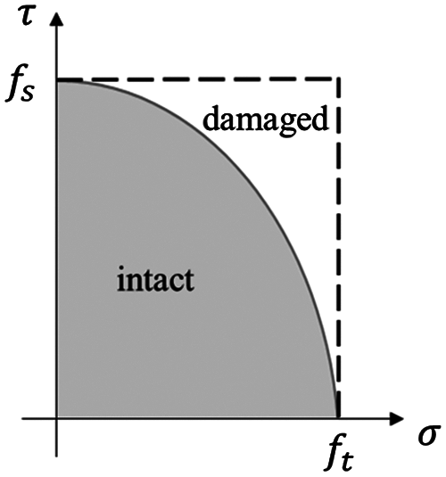
Figure 3: Hybrid failure criterion determined using normal and shear strengths

3  Validation and Analysis

The freeze bonding of the elements can transmit tension, compression, shear, bending moment, and torque. Furthermore, the motion of the elements in the bonding state should be relatively stable. Because it is difficult to identify a quantitative analysis solution for multiple elements, the bond model was validated by testing the motion of two bonded elements.

3.1 Motion Test of Bonded Elements

Two elements, bonded together as shown in Fig. 4, were used to simulate their movements, and one of them was subjected to an external force and moment. Three cases were considered corresponding to the transmissions of compression, tension, and torque. The external force and moment were perpendicular to the surface and passed through the centers of the two particles. The translational displacement and rotation angle in the moving process were recorded to verify whether the bond force transferred by the bond was corrected. The analytical solutions of the translational displacement and rotation angle of the particles were obtained according to the function as x=12(Fm)t2 and θ=12(MJ)t2, where m and J are the mass and moment of inertia, respectively. The comparison of the simulation results and analytical solutions is shown in Fig. 5, indicating that the simulation results are in good agreement with the analytical solutions.

Figure 4: External force on elements with face to face contact

Figure 5: Simulation results and analytical solutions for the elements with face to face contact (a) Translational displacement (b) Rotation angle

The postures of the two cubic elements were adjusted such that one vertex of one element was in contact with one vertex of another and their main diagonals were on the same line, as shown in Fig. 6. Similar cases were conducted to validate the bond model. The simulation results are shown in Fig. 7. These cases illustrate the effectiveness of the bond model under the vertex–vertex contact condition.

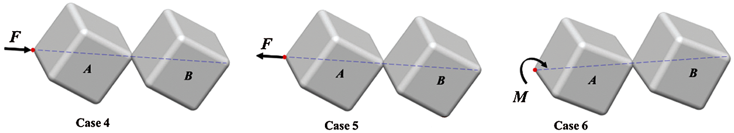
Figure 6: External force on elements with vertex to vertex contact

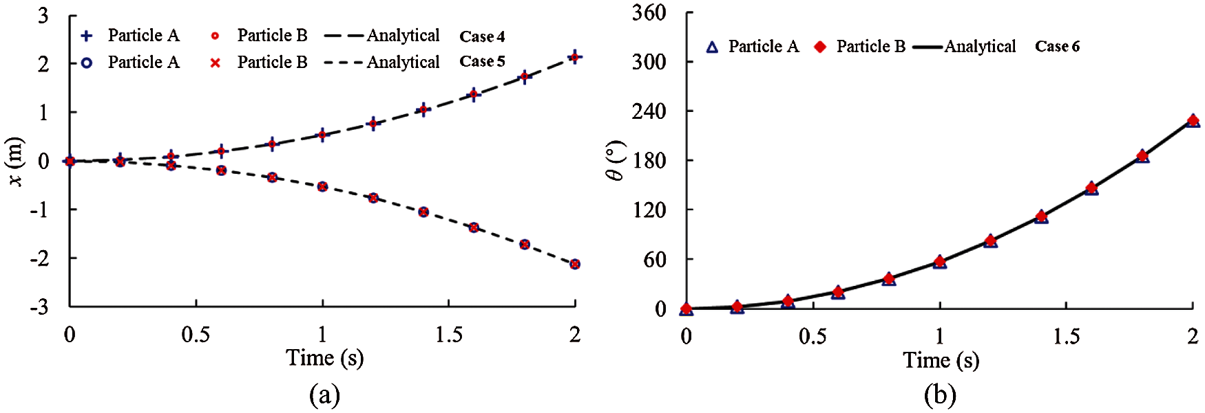
Figure 7: Simulation results and analytical solutions for the elements with vertex to vertex contact (a) Translational displacement (b) Rotation angle

3.2 Impact between the Bonded Elements and Wall

The bonding effect can sinter two elements together. For a proper bond model, no difference should exist between a single element and the bonded elements with the same geometrical features in the simulation. To validate the bond model, simulations of particles impacting on a flat static wall were conducted, where one particle was made up of a single element and another was made up of two elements bonded together, as shown in Fig. 8. The bond strength was set to a large value such that the bond did not break. No gravity and friction were considered when the polyhedral particles impacted the wall with a vertical downward translational velocity vz−. The analytical solutions of the rebound translational velocity vy+ and angular speed ωy+ can be expressed as [51]:

vz+=ωy+rcos⁡(α+θ)−evz−, (19)

ωy+=mvz−(1+e)rcos⁡(α+θ)Iyy+mr2cos2⁡(α+θ), (20)

where m is the mass of the particle; e is the restitution coefficient; α and θ are the angles between the diagonal and edge and the edge and wall, respectively, as shown in Fig. 8; Iyy is the moment of inertia about the y-axis; r is the distance between the center of the face and the corner of the face, as shown in Fig. 8. The simulation parameters are listed in Table 1.

The impact angles varied from 2° to 88°. For each impact angle (θ), the dimensionless rebound transitional velocity (vz+/vz−) and angular velocity (r ωy+/vz−) were calculated using the DEM, and a comparison with the analytical solutions is shown in Fig. 9. The results show that the bonded element corresponds with the single element, and the results also agree well with the analytical solution. The slight difference was possibly caused by the kinetic energy loss due to the deformation and damping of the bond in the calculation and can be neglected.

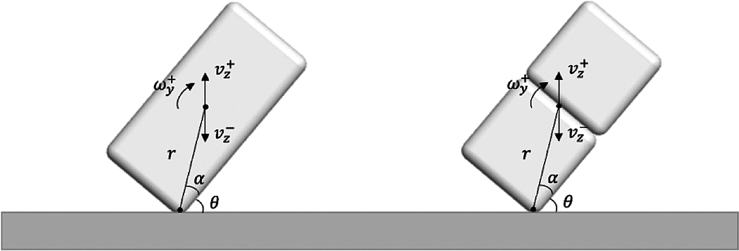
Figure 8: Sketches of single element and bonded elements impacting on the wall

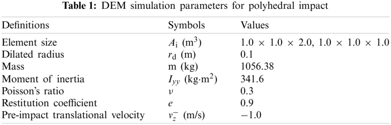
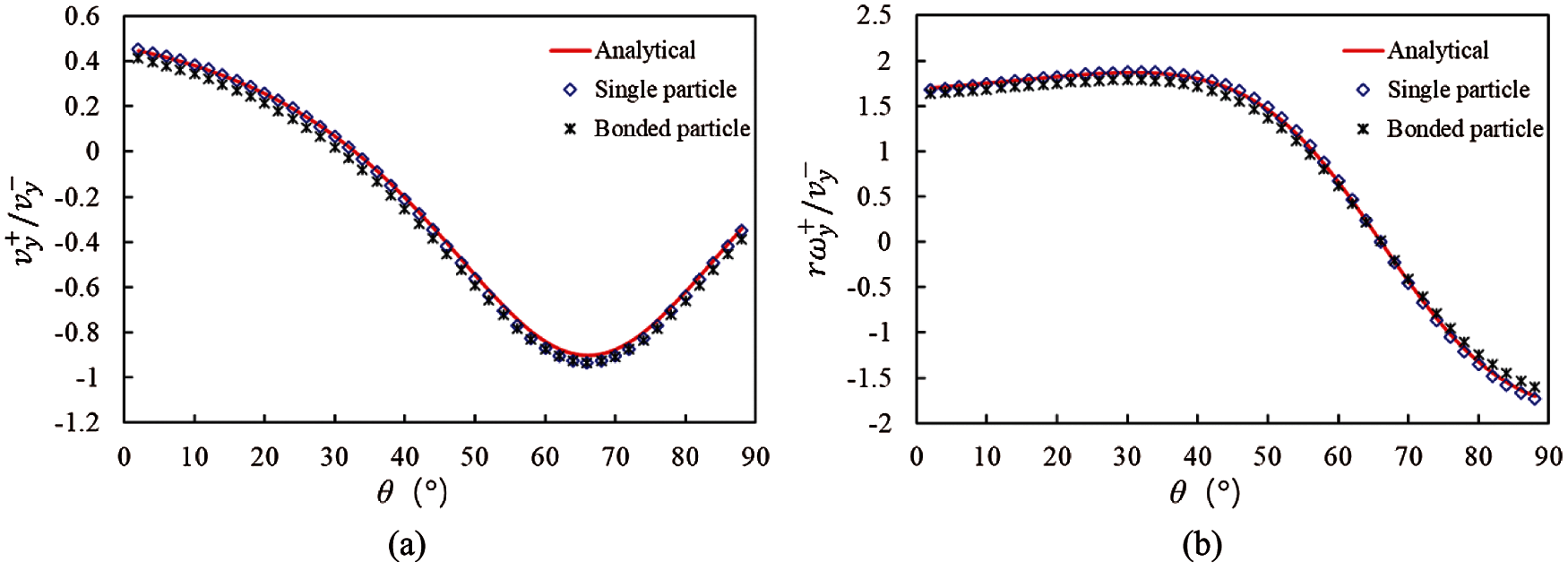
Figure 9: Dimensionless speed obtained from the analytical and simulation results (a) Translational speed (b) Angular speed

3.3 Failure of Bonded Elements

Two cases were considered to determine the failure behavior of the bond. Two cubic elements (1.0 × 1.0 × 1.0 m3) were bonded together in the simulation; one was fixed, and the other applied tensile and shear forces, increasing linearly from zero. Since the freeze-bond effect is applied at the contact point, which is obtained by the optimization model based on the approximate envelope function and has avoided the complex geometric computations of the traditional contact detection approach. The vertex-face bond, edge-face bond and vertex-edge bond are all actually point-point bond, and have no essential difference. Consequently, only the failure modes of bonds created on the contact faces of two dilated polyhedrons are verified here. The parameters considered in the simulation were: normal bonding strength ft=0.6MPa, internal cohesion C=1.8MPa, and bond area = 0.1 m2. Since bending and torsional failures are essentially due to tensile or shear forces reaching the strength, only pure tensile and pure shear simulations were studied here. Fig. 10 shows the time-history curve of the force transmitted by the bond during loading, where the results agree with the fracture criterion mentioned in Eqs. (17)–(18).

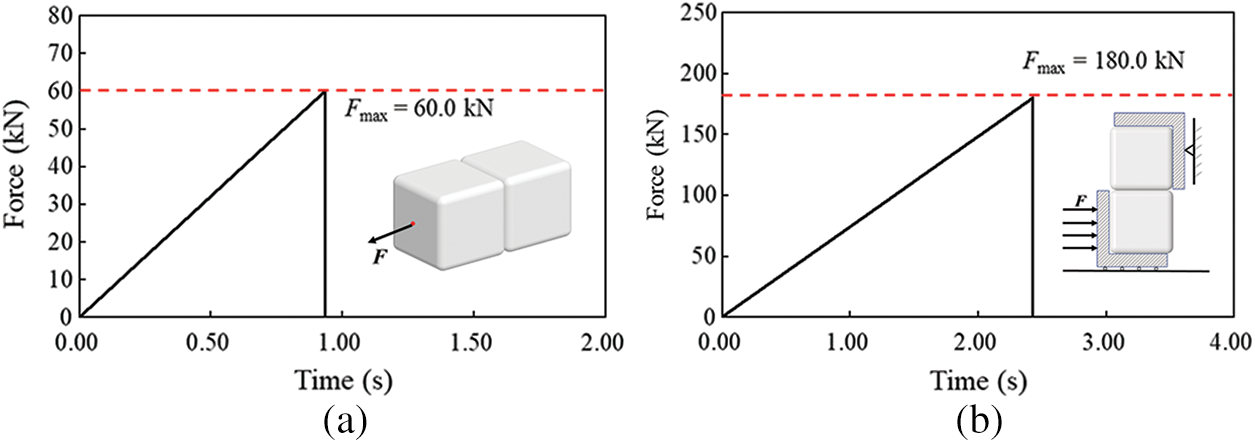
Figure 10: Force history during bonding failure (a) Tension (b) Shear

4  Simulation of the Punch-through Test of Ice Rubble

In order to study the effect of freezing on the mechanical properties of ice pile, the punch-through tests of consolidated and unconsolidated ice-rubble piles were simulated by the freeze-bond model of dilated polyhedral DEM.

4.1 Simulation Setup of Punch Test

The simulation setup refers to previous works on field punch-through experiments [23,52,53] and numerical simulation. Fig. 11 shows the simulation of the punch-through test of ice rubble. The model set consists of three parts: an indenter platen, consolidation layer, and ice rubble. The consolidated layer was like a boundary covering over the ice rubble and consisted of one-layer static ice blocks of 1.8 m × 1.8 m × 0.4 m, with the bottom fixed at z = −1 m. A circular hole was provided at the center for the indenter to press down. An ice-rubble pile floated under the consolidated layer. To construct the ice rubble, two sizes of ice blocks were used, 1.8 m × 1.8 m × 0.4 m and 0.6 m × 0.6 m × 0.4 m. A circular flat indenter with a diameter wI was moved down vertically into the ice rubble, its reactive force F and displacement δ were recorded, and the buoyancy on the indenter was ignored.

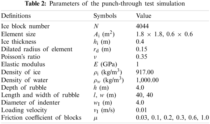
Initially, the bottom of the indenter was slightly higher than the bottom of the consolidated layer, trying not to touch the ice blocks. A total of 4,404 ice blocks of two sizes with random positions, orientations, and translational and rotational velocities were released underwater in a pool of 40 m × 40 m and allowed to float with their buoyancy until they remained static beneath the consolidated layer. Fig. 12 shows the initial state of the DEM simulation, where the red portion represents the consolidated layer and the ice rubble mass is displayed in green and blue layers according to the vertical position for better display of the relative movement of ice blocks. The initial thickness of the ice rubble was h = 4 m, and the length and width were l = w = 40 m. The ice rubble is surrounded by four vertical fixed walls, whose friction coefficients are set as zero. The rubble length and width are enough to ensure that the punching process and force exerted on the wall were not affected by wall constraints. The porosity of the initial ice rubble was approximately 51.55%, and the main parameters of the simulation are listed in Table 2. Following the work of Heinonen [23], the indenter had a diameter of 4 m and thickness of 1.0 m and moved downward vertically with a constant velocity of 0.01 m/s.

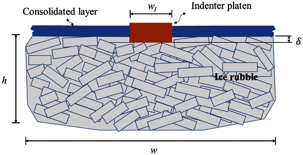
Figure 11: Sketch of punch-through test for ice rubble

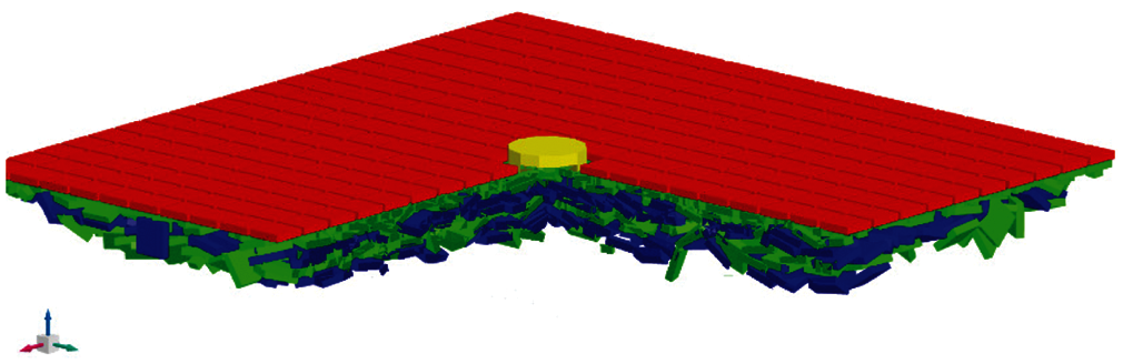
Figure 12: DEM model of punch-through test

4.2 Punch-through Test of the Unconsolidated Ice Rubble

The effect of freezing on the mechanical properties of ice rubble was studied by comparing the punch-through test results of the unconsolidated and consolidated ice rubble. This section presents the results for unconsolidated ice rubble; the process is shown in Fig. 13, and the friction coefficient used is 0.03. As the indenter penetrated, the ice blocks beneath the indenter were squeezed, resulting in their vertical downward displacement, and the ice blocks near the edge of the indenter also slipped.

Fig. 14 shows the force–displacement curve of the indenter from the simulation of the unconsolidated ice rubble. According to the characteristics of the curve, the punch-through test was divided into four stages:

In Stage I, with the penetration of the indenter, the indenter resistance initially increased rapidly until the force reached a maximum value of approximately 54 kN. At δ = 200 mm, a sudden drop in the force occurred, which was caused by the release of shape interlocking and redistribution of inter-particle forces within the rubble at this time. The subsequent loading made the ice recompact, and then the resistance of the indenter continued to rise.

In Stage II, the resistive force remained at an approximately constant level after reaching the maximum value. The relative displacement between the ice blocks in the ice rubble was small, and no large movement occurred. The ice block at the lower edge of the indenter tilted slightly but did not deviate from the pressure range of the indenter. Fmax is the average value of the force at this stage, which characterizes the overall mechanical properties.

In Stage III, resistance reduction occurred. The indenter continued to penetrate the internal structure of the ice rubble, and the ice blocks below moved downward; in addition, the ice blocks at the edge of the indenter bottom also underwent a tangential relative displacement with respect to the ice beneath the indenter, and the interlocking effect was broken gradually. This stage can be regarded as the stage of shear failure of the entire structure.

Stage IV is the equilibrium stage after punching through, at which the resistance force of the indenter was mainly derived from the buoyancy of the residual ice blocks below.

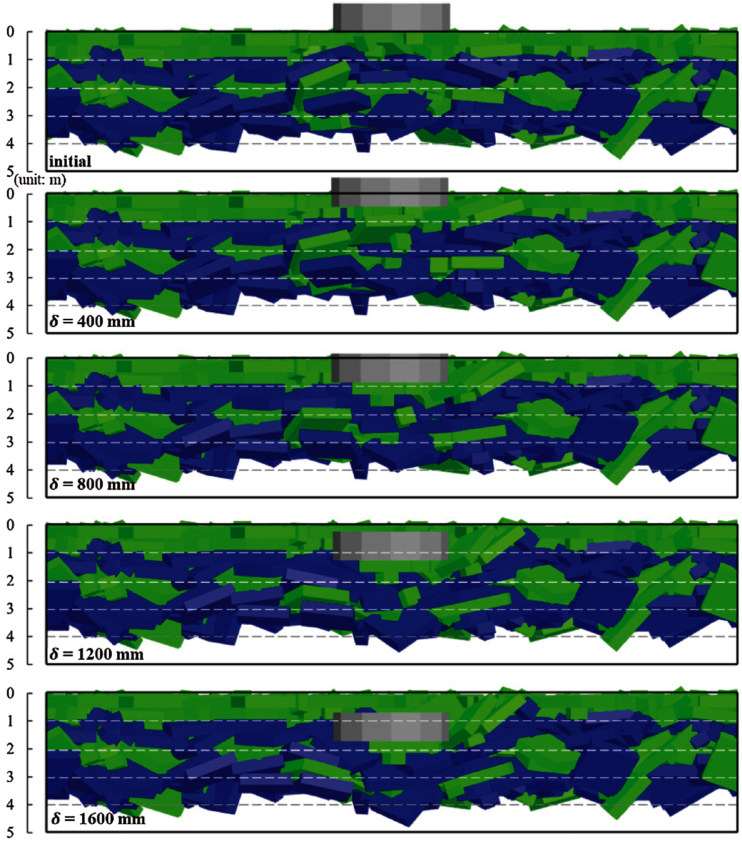
Figure 13: Simulation results of punch-through test of unconsolidated ice rubble

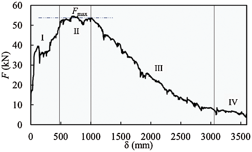
Figure 14: Force–displacement curve for the test on unconsolidated ice rubble

In the process of indenter penetration, the displacement of the ice blocks can be divided into vertical movement that follows the downward movement of the indenter and horizontal movement from the center to periphery. The two types of displacement distributions are shown in Fig. 15. The relative displacement shown in color is dimensionless (calculated as displacement of ice blocks divided by displacement of indenter) to better represent the movement. As observed, the ice blocks mainly moved vertically, and the magnitude of lateral movement was small relative to the vertical movement (Note: the upper limits for the scales in Figs. 15a and 15b differ by a factor of two). The ice blocks directly beneath the indenter mainly moved vertically, while the peripheral ice near r = 2 m mainly moved horizontally to the outside.

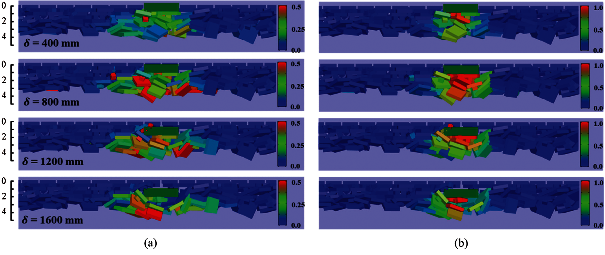
Figure 15: Movement of ice blocks during the punch-through test (a) in lateral direction and (b) in vertical direction

4.3 Punch-through Test of the Consolidated Ice Rubble

The same initial ice rubble, as described earlier in Section 4.1, was used to apply the cohesion between the ice elements. The calculation parameters of this simulation are listed in Table 3, and the other parameters are consistent with those in the above case. In natural ice rubble, since the frozen face size has a random and inconsistent distribution, it is difficult to make a calibration while studying ice freezing behavior. Therefore, to simplify the setting, the bonding face area between the ice elements and bond strength in the simulation were assumed to have constant values.

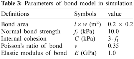
Fig. 16a shows the force–displacement curve of the indenter for the punch-through test performed on consolidated ice rubble, and Fig. 16b shows an enlarged version of Fig. 16a for the initial range of indenter penetration. According to the characteristics of the force–displacement curve, the punching process can be divided into three stages, as shown in Fig. 16b. Stage I is the initial stage of penetration, where the resistance increased rapidly with the downward movement of the indenter and quickly reached the peak value Fmax. In Stage II, the indenter resistance decreased rapidly, and the ice rubble entered the overall failure stage. In the micro view, a large number of bonds in the ice body were broken, and in the macro view, it was the shear failure of the entire ice rubble. At this stage, the strength of the ice rubble mainly depended on the freeze bond between ice blocks, rather than interlocking and tangential friction. In Stage III, most bonds on the shear plane failed, and dislocations occurred in the ice rubble. The major factors controlling the stiffness of ice rubble were interlocking and friction. Furthermore, the fluctuations in the curve corresponded to slip and recompaction between ice blocks. After this stage, the phenomenon was similar to that of unconsolidated ice rubble. Moreover, it did not affect the overall strength; thus, details have not been provided.

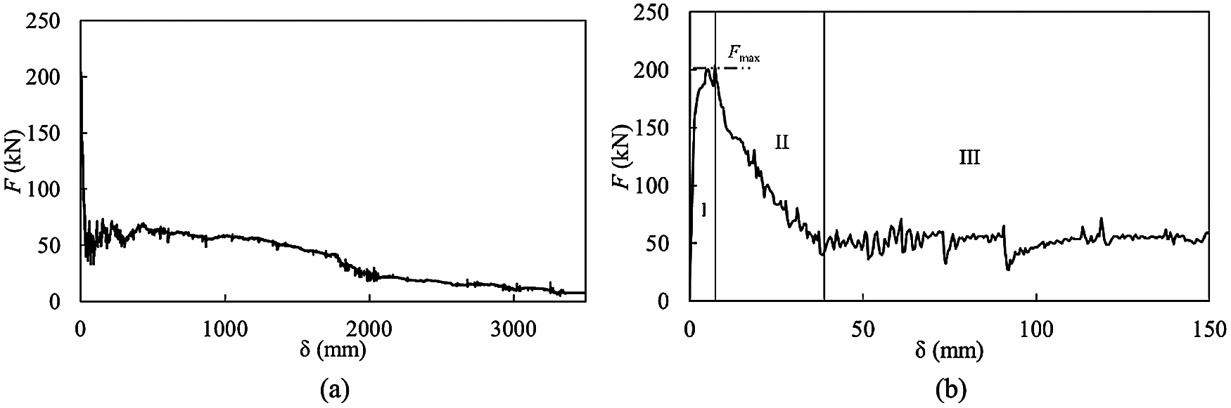
Figure 16: Force–displacement curve for the test on consolidated ice rubble (a) δ = 0–1000 mm (b) δ = 0–150 mm

Fig. 17 shows the ice blocks’ vertical displacement (dimensionless) distributions during the penetration process at each stage. Because the horizontal displacement was not apparent at the early stage, it is not presented. Accordingly, Fig. 18 shows the number of cohesive bonds broken and the breaking rates in the three stages. It can be observed that the deformation in the ice rubble was small in Stage I, and the internal force increased continuously, but there were few bond fractures. Therefore, the ice rubble was a complete structure with little damage at this stage. In Stage II, both the number of failed bonds and failure rate were the highest among the three stages, which indicated that the failure of the internal bonds was very severe at this stage. The resistance of the indenter also decreased rapidly with the fracture of a large number of bonds, which verifies that freeze bonding plays a crucial role in the overall strength of the ice rubble. After the breakage of the majority of the bonds, the ice rubble deformed more significantly than that in Stage I, and the general failure occurred. In Stage III, ice blocks beneath the indenter moved down as a whole after compaction. The bond failure rate also decreased, which indicates that it mainly depended on the interlocking effect and friction to resist the deformation. All the results corresponded well to the force–displacement curve of the indenter and explained the failure mechanism of the ice rubble.

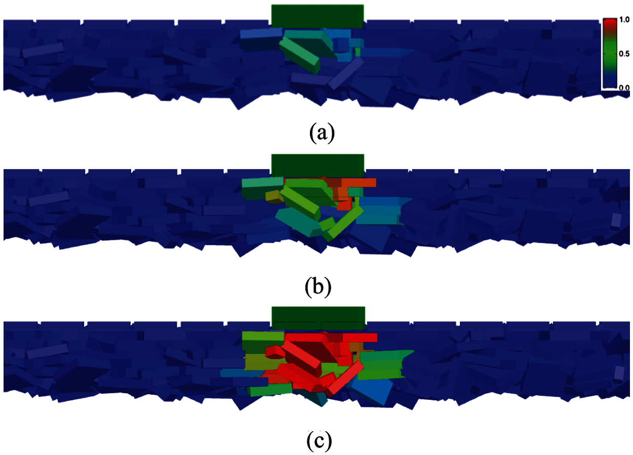
Figure 17: Movement of ice during the punch-through test for consolidated ice rubble (a) Stage I (b) Stage II (c) Stage III

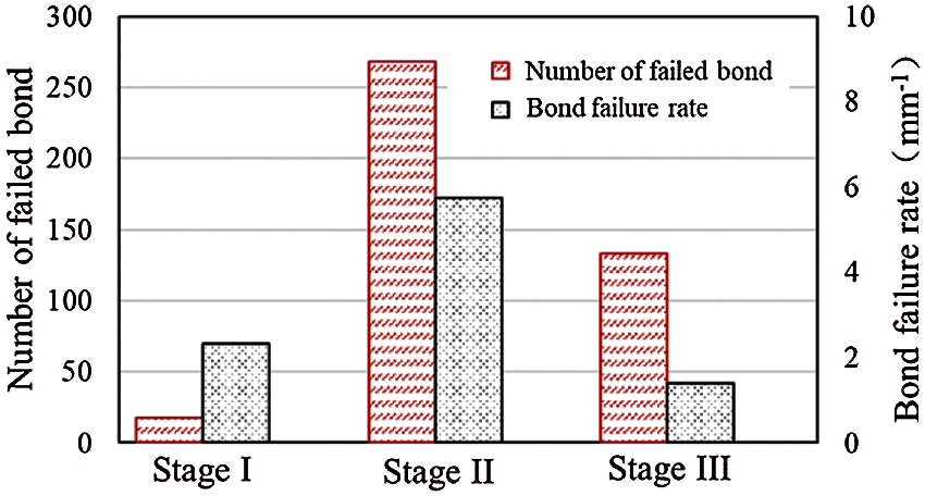
Figure 18: Bond failure process during the punch-through test for the consolidated ice rubble

The DEM simulation results were compared with the experimental results of Helnonen’s work on the in-situ punch-through test of an ice ridge [23], as shown in Fig. 19. As shown, significant uncertainty was observed in the experiment, but the general trend of the curve could explain the failure process of the ice rubble. The DEM simulation and experimental results agreed well in Stage I and Stage II; however, the differences between the results in Stage III may be due to the differences between the initial ice rubble properties, i.e., the porosity, internal friction, geometry, and size of the ice blocks. Through this comparison, the DEM bond model was also validated.

4.4 Comparison of Results of Unconsolidated and Consolidated Ice Rubble

Comparing the force–displacement curves of unconsolidated and consolidated ice rubble (Figs. 14 and 16b), it is observed that the consolidated ice rubble exhibited higher strength and larger stiffness. In addition, comparing the overall failure stages of the curves, it can be observed that the force drop of the frozen ice rubble was steeper than that of the nonfrozen ice rubble, and the frozen ice rubble exhibited clearer brittleness characteristics than that of the nonfrozen ice rubble.

In the first three stages of the unconsolidated ice rubble, the strength and stiffness of the ice rubble were mainly provided by the interlocking and tangential friction between the ice blocks. When the indenter was pressed down, the ice blocks moved and adjusted their positions to adapt to the higher pressure. Therefore, the resistive force did not increase or decrease immediately as the indenter penetrated; thus, the unconsolidated ice rubble can be considered to have the characteristics of a relative ductile failure. In the first and second stages of the consolidated ice rubble, the main structural strength of the consolidated ice rubble was provided by the freeze bonding between the ice blocks. At the initial stage of pressing the indenter, the ice rubble can be regarded as a complete structure, and the ice did not dislocate relatively. Therefore, the indenter resistance increased rapidly during loading. When the maximum force was reached, the local freeze bond could not bear the large deformation, and failure occurred. The failure of the local bond reduced the overall strength of the consolidated ice rubble rapidly. This type of failure is largely similar to brittle failure.

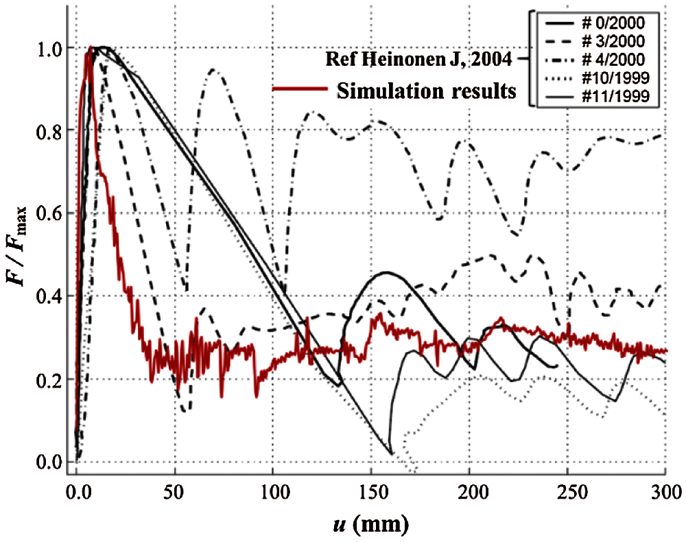
Figure 19: Dimensionless force–displacement comparison between simulation and in-situ test

According to the deformation and failure process of the ice rubble, the shear plane of the ice rubble failure was assumed to be a cylindrical surface, which can be defined by the perimeter of the indenter platen and rubble thickness [23]. Therefore, the effective shear strength of the ice rubble can be expressed as:

τ=FmaxπwIh, (21)

where Fmax is the maximum resistance of the indenter during penetration, and wI and h are the diameter of the indenter and thickness of the ice rubble, respectively.

To investigate the effect of the friction coefficients μ on the shear strength, punch-through tests of consolidated and unconsolidated ice rubble under six different friction coefficients were simulated, and the results are shown in Fig. 20. The results show that for any friction coefficient, the shear strength of consolidated ice rubble is larger than that of unconsolidated ice rubble. In addition, the friction coefficient has a significant influence on the shear strength of unconsolidated ice rubble but has little effect on consolidated ice rubble. As mentioned above, the shear strength of consolidated ice rubble is mainly related to the strength of the freeze bonding but not to the friction coefficient. However, for unconsolidated ice rubble, the shear strength is mainly affected by the interlocking effect and shear friction between the ice blocks. Consequently, as the friction coefficient increases, the shear strength shows an approximate linear increase.

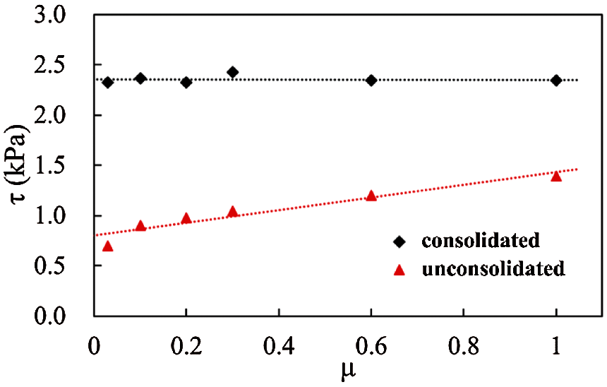
Figure 20: Effect of friction coefficient on shear strength of ice rubble

5  Conclusions

In this study, a freeze-bond model based on the dilated polyhedral DEM was developed to model the freeze bonding in ice rubble. This paper includes the methodology, verification, and application of the model to simulate the punch-through test of unconsolidated and consolidated ice rubble. The DEM polyhedral elements could be bonded together by establishing an imaginary bonding surface and bonding point to transfer the force and moment between the freezing elements. The failure process of the freeze bonding adopted the mixed fracture criterion considering the tensile and shear strengths together. The bonding effect between the two freezing elements and the fragmentation behavior were simulated, and the accuracy and stability of the model were verified.

The proposed bond model of the DEM polyhedral elements was used to simulate the punching process of the ice rubble, and the macroscopic mechanical properties of the ice rubble under nonfreezing and freezing conditions were considered. The resistive force–displacement curve of the indenter and movement of the individual ice blocks were analyzed. In conclusion, the strength and stiffness of the ice rubble increase under freezing and the resistance to deformation mainly depends on the freeze bond effect between ice blocks. Moreover, under nonfreezing conditions, the overall strength mainly depends on the interlocking and friction between the elements.

Frozen face size indeed has a random and inconsistent distribution in the ice rubble, however, there are few works on the relationship between freezing degree and bonding area. Besides, the freezing degree is also dominated by environmental conditions. Further work on the calibration of bond parameters needs to be organized and the quantitative relationship between the parameters of the DEM bond model and the mechanical properties of the frozen bond in specific environmental conditions should be established by the lab and in situ experiments.

Funding Statement: This study was financially supported by the National Key Research and Development Program of China (Grant No. 2018YFA0605902), the National Natural Science Foundation of China (Grant Nos. 20212024, 11872136) and China Postdoctoral Science Foundation (Grant No. 2020M670746).

Conflicts of Interest: The authors declare that they have no conflicts of interest to report regarding the present study.

This work is licensed under a Creative Commons Attribution 4.0 International License, which permits unrestricted use, distribution, and reproduction in any medium, provided the original work is properly cited.