Computer Modeling in Engineering & Sciences

DOI: 10.32604/cmes.2022.018113

ARTICLE

Dynamic-Response Analysis of the Branch System of a Utility Tunnel Subjected to Near-Fault and Far-Field Ground Motions in Different Input Mechanisms

Yuhang Jin1,2, Endong Guo1,2,*, Houli Wu1,2 and Peilei Yan1,2

1Institute of Engineering Mechanics, China Earthquake Administration, Harbin, 150080, China
2Key Laboratory of Earthquake Engineering and Engineering Vibration, Harbin, 150080, China
*Corresponding Author: Endong Guo. Email: iemged@263.net
Received: 30 June 2021; Accepted: 07 September 2021

1  Introduction

Currently, traffic jams and the lack of public space caused by the old urban form have greatly restricted the development of cities. Among the numerous reconstruction schemes, the urban underground space has been considered to play an effective role in urban renewal [1]. As an important infrastructure in the urban underground space, utility tunnels refer to the underground construction of a tunnel space that integrates electricity, communication, water-supply, and drainage, among other municipal pipelines. In addition, these tunnels are equipped with ventilation shafts and a pipeline branch system to realize unified construction and management [2]. However, there are many kinds of pipelines in a utility tunnel, which may lead to multi-hazard coupling disasters, causing severe economic losses and heavy casualties. Compared with the low-impact high-probability characteristics of the traditional buried-pipeline accident, a utility-tunnel accident has the characteristics of high-impact and low-probability [3]. Soil liquefaction occurred during the Niigata earthquake in Japan in 1964, which caused the whole tunnel to float up, and soil flowed into the tunnel [4]. The Miyagi earthquake in 1971 caused the interface to break and the tunnel to crack, and it damaged the water supply, drainage, and gas supply pipelines [5]. The 1994 Northridge earthquake in the United States caused the explosion of a gas pipeline and damaged the tunnel [6]. Unfortunately, earthquakes are one of the main reasons for the damage to underground structures. The current code for utility tunnels does not provide a clear seismic design method, which needs to be solved urgently.

Seismic analysis methods of underground structures can be divided into quasi-static analyses and time-history analyses [7]. The calculation process of the pseudo-static analysis method is relatively simple and is suitable for practical engineering structures with simple cross-section forms. Common quasi-static analysis methods such as the response-deformation method, which uses a soil spring to replace the soil around the structure, can achieve better calculation accuracy for simple-structure systems. Liu et al. [8] proposed an integral response-deformation method, which was in good agreement with the dynamic time-history analysis method when calculating the standard section of a two-dimensional subway station. The time-history analysis method can also achieve high accuracy for complex structural systems, but the calculation cost is high, and it has high requirements for the treatment of the soil-structure interface, the selection of an artificial boundary, and the input of ground motion. Sun et al. [9] established the structure-soil-spring coupling finite element model and used the contact pair to simulate the soil-structure interaction.

In recent years, research on the dynamic response of near-fault earthquakes and far-field earthquakes has mainly focused on the above-ground structure [10–12]. Only a few scholars have studied the underground tunnel. Mei et al. [13] proposed a new velocity-pulse equivalent model to explain the seismic response of a tunnel during near-fault pulse ground motion; Yu et al. [14] developed an analytical solution for a deep-buried circular tunnel covered by an isolation layer that was subjected to far-field shear stresses; Sun et al. [15] evaluated the seismic response and damage degree of a hydraulic-arch tunnel under a near-fault SV wave and compared the effects to a probabilistic seismic response with far-field ground motion; Yang et al. [16] studied the dynamic response of a tunnel in sand under near-fault ground motion by using a 1 g shaking-table test. However, the traditional tunnel is quite different from the utility tunnel in terms of buried depth, site conditions, and structural form. Therefore, it is necessary to study the seismic response of the utility tunnel to near-fault and far-field ground motions.

Based on the popularization of utility tunnels in the urban underground space and many damage cases of utility tunnels due to earthquakes, the seismic performance of utility tunnels has attracted the attention of scholars. The current seismic research on utility tunnels has mainly focused on the standard segment of the utility tunnel. Through time-history analysis, Jiang et al. [17] obtained the weak position of an urban underground pipe gallery when it was damaged. Chen et al. [18] carried out a shaking-table test on a model of a utility tunnel with construction joints and obtained the relationship between the dynamic response and the peak acceleration of the utility tunnel. Some scholars also focus on the seismic performance of the joints of the utility tunnel, but most of them do not consider the internal pipes. Pan et al. [19] studied the mechanical performance of an L-shaped joint under different loads using a shaking-table test and finite element analysis. A few scholars have considered the pipelines in the utility tunnel in the seismic analyses, but the section form of the utility tunnel was simple [20–22].

At present, the seismic research on utility tunnels is mostly concentrated on the standard section, and the related research on pipelines in the tunnels is less common. Additionally, the research form is relatively narrow, which is not enough to meet the development trend of the diversified structure of utility tunnels, the integrated construction of underground spaces, and the changing social needs [23–25]. However, as an important joint of a utility tunnel, the branch system is a weak link in the seismic design of the whole utility tunnel due to the sudden changes of the section form. Once the tunnel is damaged under an earthquake’s action, it will inevitably lead to a domino effect, resulting in damage to the internal pipeline, leading to the leakage of liquid or gas, which will lead to serious secondary disasters.

To study the seismic response of complex underground structures such as the branch system, an input model of the ground motion is explained in Section 2, which includes the viscous-spring artificial-boundary theory and the deduction of an equivalent nodal force when the P wave and SV wave are vertically incident. Section 3 presents a finite element model in ABAQUS software, including the model size, constitutive relation, implementation of the artificial boundary, and equivalent nodal force in the software. In Section 4, the selected near-fault and far-field ground motions are described. Section 5 presents the comparison of the dynamic response of the branch system of a utility tunnel subjected to different ground motions in different input mechanisms as well as a series of seismic analyses. Finally, the conclusion of this study is presented in Section 6.

2  Ground Motion Input Model

2.1 Three Dimensional Viscous-Spring Artificial Boundary Theory

To ensure the calculation accuracy of the soil-structure interaction, a viscous-spring artificial boundary was used to simulate the infinite field. This was achieved using a parallel system of spring-dampers on the intercepted soil boundary nodes, which were used to simulate the elastic-recovery capacity of a semi-infinite medium, consume the ground-motion energy, and overcome the low-frequency global drift [26]. The spring stiffness and damping coefficients of the artificial boundary were determined by the soil properties, and the calculation formula is as follows [27,28]:

KBN=αNGR,CBN=ρCp, (1)

KBT=αTGR,CBT=ρCs, (2)

where KBN and KBT are the normal and tangential spring-stiffness coefficients, respectively, CBN and CBT are the boundary normal and tangential damping coefficients, respectively, G is the shear modulus, ρ is the foundation density, and R is the distance from the wave source to the artificial-boundary node. Generally, the distance from the geometric center of the ground surface to the side boundary can be approximately taken for four side boundaries, and the distance from the geometric center to the bottom boundary is approximately taken for the bottom boundary. Cp and Cs are the velocities of the P wave and S wave, respectively, and αN and αT are the normal and tangential artificial-boundary coefficients, respectively, and their values need not be fixed. Good results can be obtained in a certain range [11], and in this paper, αN = 1.33 and αT = 0.67.

According to the elastic formula, the shear modulus G can be expressed by the elastic modulus E and Poisson’s ratio ν:

G=E2(1+ν). (3)

The velocities of the P and S waves are defined as follows:

Cs=Gρ=E2ρ(1+ν), (4)

CP=λ+2Gρ=E(1−ν)ρ(1+ν)(1−2ν). (5)

For node b, shown in Fig. 1, the spring-stiffness coefficients and damping coefficients in Eqs. (1) and (2) needed to be multiplied by the influence area of node b to obtain the spring stiffness and damping values of node b. The influence area of a node is equal to the total area of the elements around the node divided by the number of elements around the node.

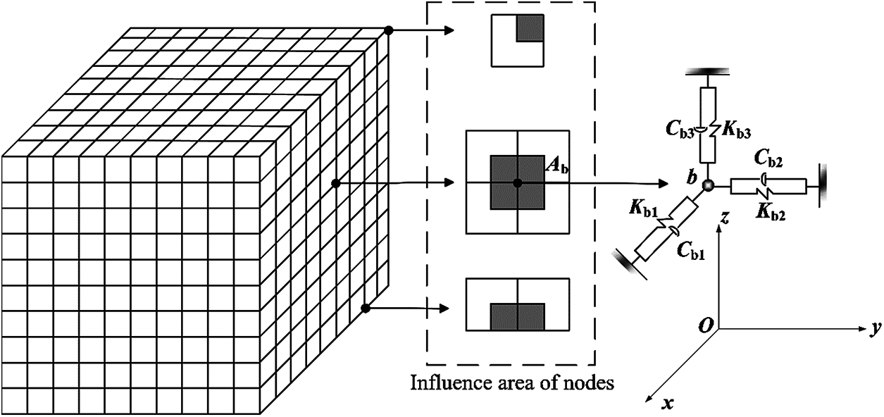
Figure 1: The sketch of the viscous-spring boundary

2.2 Equivalent Nodal Force Theory

This paper refers to the method of Liu et al. [29]. Transforming a seismic-wave input into a wave-source input enables free-field motion of the boundary nodes, such that the ground motion can be input into the finite element model in the form of a concentrated force at the boundary nodes. For the boundary node b, the equivalent nodal force is:

Fb=(KbUbf+CbU˙bf+σbfn)Ab={FbxFbyFbz}, (6)

where Ubf=[u,v,w]T, U˙bf=[u˙,v˙,w˙]T, and σbf are the displacement vector, velocity vector, and stress tensor of the free field of boundary nodes, respectively, n is the normal cosine vector of the boundary surface where node b is located, and Ab is the influence area of the node.

Since the incident angle of the seismic wave is nearly perpendicular to the surface when it reaches the ground surface, according to the geometric and physical equations of elastic mechanics:

εxx=0,εyy=0,εzz=∂w∂z,εxy=0,εyz=∂v∂z,εzx=∂u∂z, (7)

{σxxσyyσzzσyzσzxσxy}=[λ+2Gλλλλ+2Gλλλλ+2GGGG]{εxxεyyεzzεyzεzxεxy}={λ∂w∂zλ∂w∂z(λ+2G)∂w∂zG∂v∂zG∂u∂z0}. (8)

The free-field stress tensor can be obtained as follows:

σbf=[λ∂w∂z0G∂u∂z0λ∂w∂zG∂v∂zG∂u∂zG∂v∂z(λ+2G)∂w∂z]=[λ∂w∂z0ρCs2∂u∂z0λ∂w∂zρCs2∂v∂zρCs2∂u∂zρCs2∂v∂zρCp2∂w∂z], (9)

where λ is the lame constant.

In this paper, the P wave and SV wave are vertically incident at the same time; Ubf=[u(t),v(t),w(t)]T, and U˙bf=[u˙(t),v˙(t),w˙(t)]T. Therefore, according to one-dimensional wave theory:

∂u∂z=−1Cs∂u∂t,∂v∂z=−1Cs∂v∂t,∂w∂z=−1Cp∂w∂t. (10)

We can obtain:

σbf=[−λCp∂w∂t0−ρCs∂u∂t0−λCp∂w∂t−ρCs∂v∂t−ρCs∂u∂t−ρCs∂v∂t−ρCp∂w∂t]. (11)

When node b is located on the artificial boundary of the bottom surface:

Ubf={u(t)v(t)w(t)}={u0(t)+u0(t−2HCs)v0(t)+v0(t−2HCs)w0(t)+w0(t−2HCp)}. (12)

When node b is located on the artificial boundary of the side surface:

Ubf={u(t)v(t)w(t)}={u0(t−hCs)+u0(t−2H−hCs)v0(t−hCs)+v0(t−2H−hCs)w0(t−hCp)+w0(t−2H−hCp)}, (13)

where h is the distance from b to the artificial boundary, and H is the distance from the bottom artificial boundary to the ground surface.

3  Finite Element Model

The branch system is the part where the internal pipeline and external pipeline of a utility tunnel are connected. The tunnel section is partially expanded, and either the roof is partially raised or the floor is lowered locally. In this paper, the branch system of a utility tunnel in Nanjing was taken as the research object, and nonlinear dynamic-response analysis was carried out to study the seismic characteristics of the branch system in different ground-motion input mechanisms.

3.1 Geometric Parameters of the Model

Due to the large scale of the utility tunnel in the longitudinal direction, in order to save calculation costs, the 3D time-history analysis cannot be modeled completely according to the original longitudinal dimension. In fact, when the longitudinal dimension is larger than a certain length (75–100 m), the influence of the longitudinal boundary condition on the structural response is weakened [22,30]. In this paper, the longitudinal length was 100 m. The reinforcement drawings of the standard segment and branch joint of the utility tunnel are shown in Figs. 2–7. The unmarked steel bars in the drawing are 28 mm in diameter and 150 mm in spacing.

The pipeline route is shown in Fig. 8. The diameter of the internal pipeline of the utility tunnel is 800 mm, and the diameter of the buried pipeline of the outgoing line is 500 mm. The pipeline in the tunnel is provided with a pier every 6 m. The width in the Y-direction and the depth in the Z-direction are 42 and 20 m, respectively. The upper part of the branch system of the pipeline is covered with 0.5 m of soil, and the buried depth of the outlet pipeline is 1.75 m.

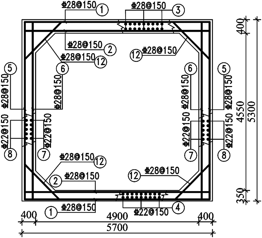
Figure 2: Cross-section Ⅰ size and reinforcement drawing

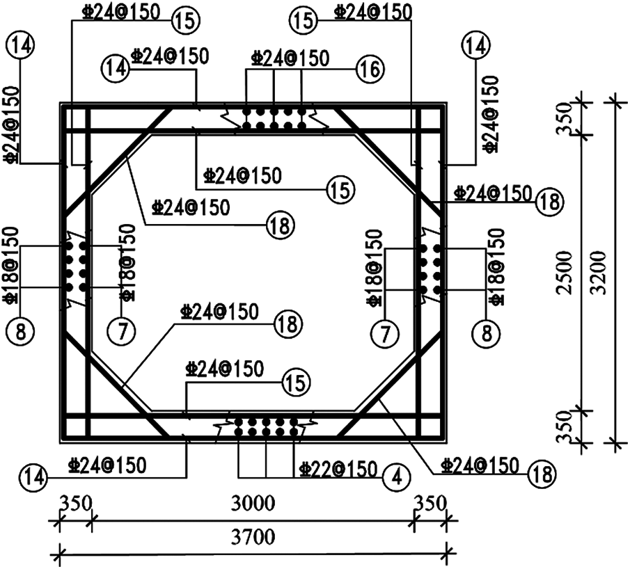
Figure 3: Cross-section ⅠⅠ size and reinforcement drawing

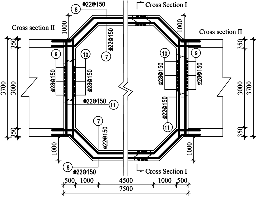
Figure 4: Plane reinforcement drawing of the branch joint of a utility tunnel

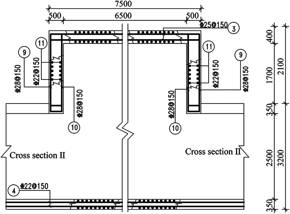
Figure 5: Elevational reinforcement drawing of the branch joint of a utility tunnel

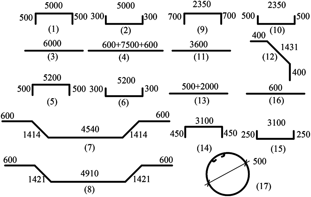
Figure 6: Master drawing of reinforcement

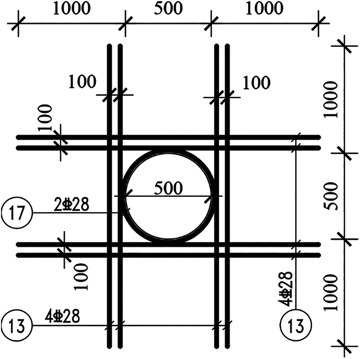
Figure 7: Branch joint opening size and reinforcement

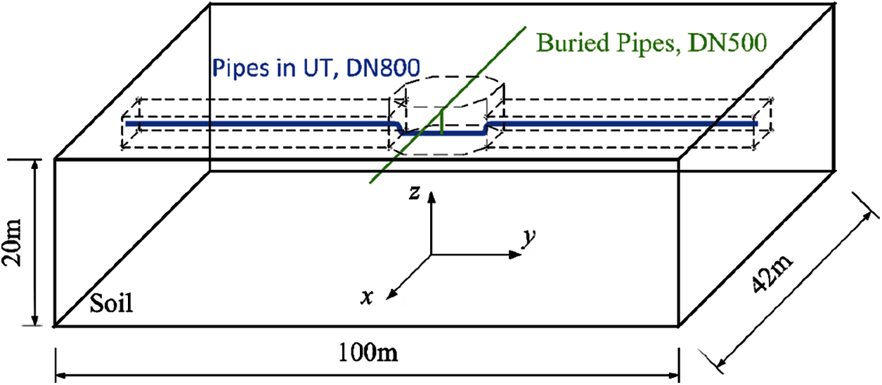
Figure 8: Drawing of pipeline route

3.2 Material Properties

The plastic-damage model [31,32] was adopted in the utility tunnel to simulate concrete damage. It was assumed that the strain can be decomposed into:

ε=εe+εp, (14)

where εis the total strain tensor, εe is the elastic part of the strain tensor, and εp is the plastic part of the strain tensor.

The stress-strain relations can be expressed by stiffness degradation and the elastic part of the strain tensor:

σ=(1−d)D0e:(ε−εp)=(1−d)σ¯,σ¯=D0e:(ε−εp), (15)

where σ is the stress, and d is the scalar stiffness-degradation variable that has a value that varies from 0 to 1, and concrete cracking or crushing will lead to the change of d. D0e is the initial elastic stiffness (undamaged stiffness), and σ¯ is the effective stress.

For any section, (1 – d) represents the proportion of the effective area of load-carrying to the total cross-sectional area, that is, the undamaged effective section bears the load after the concrete cross-section is damaged, so as to establish a plastic formula for the effective stress.

The equivalent plastic strain ε˜p consists of two independent variables: the tension part ε˜tp and the compression part ε˜cp. The degradation response of concrete is also controlled by two independent uniaxial stiffness-degradation variables, dt and dc; the effective uniaxial cohesion stress can be expressed as follows:

{σ¯t=σt(1−dt)=E0(εt−εtp)σ¯c=σc(1−dc)=E0(εc−εcp), (16)

where E0 is the initial elastic stiffness.

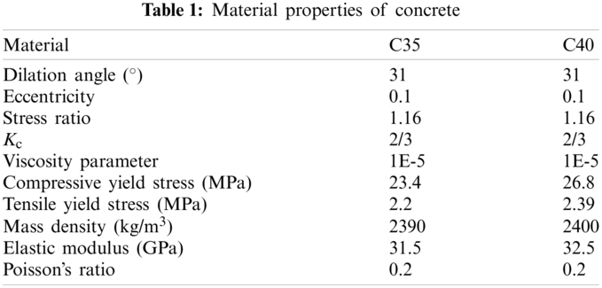
In this paper, C35 concrete was used for the main structure and piers of the utility tunnel, a concrete casing was set at the branch-joint opening, and C40 concrete was used for simulation. From the Chinese Code [33], the specific material properties are presented in Table 1, and the yield stress-cracking strain curve and the damage factor-cracking strain curve of concrete are shown in Fig. 9.

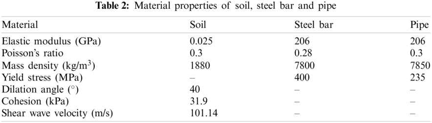
According to the report of the geotechnical investigation, the soil in this area is mainly silty clay. The Drucker–Prager failure criterion was used for the soil, Q235 steel was used for the pipe, and HRB400 steel was used for the steel bar. The specific properties are presented in Table 2.

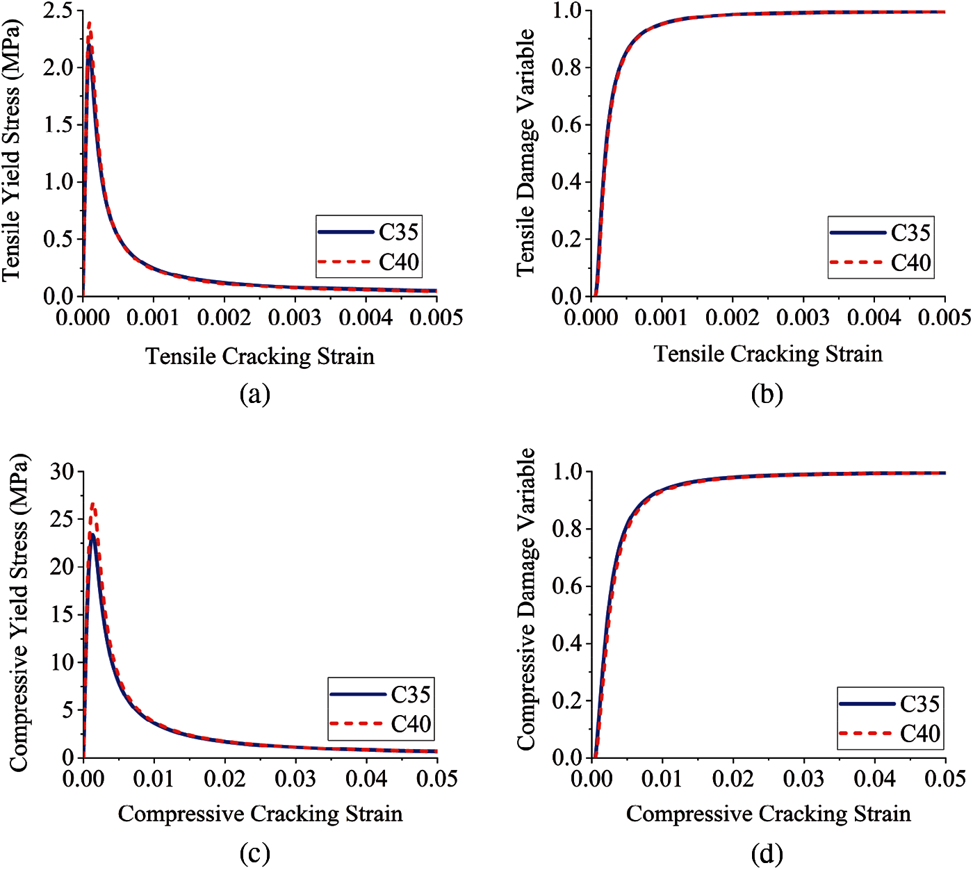
Figure 9: Mechanical behavior curve of concrete (a) Tensile yield stress-tensile cracking strain curve (b) Tensile damage variable-tensile cracking strain curve (c) Compressive yield stress-compressive cracking strain curve (d) Compressive damage variable-compressive cracking strain curve

3.3 Details of the Model

In this paper, ABAQUS software was used for modeling. To ensure the accuracy of the ground-motion input, the size of the finite element mesh was limited to a certain extent. However, the finer the mesh is, the higher the cost of the calculation will be. Element mesh size is generally determined by the seismic wavelength, such that d/λmax≤1/20. In other words, the mesh size d is determined by the wavelength of the highest-frequency component of the ground motion [34].

The soil was simulated by a solid element (C3D8R), and the mesh size was 1 m × 1 m × 1 m, which was refined near the branch joint and the buried pipeline. For the utility tunnel, this paper mainly studied the branch joint. Therefore, the branch joint was divided by the solid element (C3D8R), and the standard segments on both sides of the branch joint were divided by the continuous shell element (SC8R). At the same time, the steel bars were embedded in the concrete without considering their bonding slip. The pipe was simulated by a shell element (S4R), and the piers were poured with plain concrete, which was divided by solid elements.

In practical engineering, the pipe is completely fixed on the piers by a steel hoop; so, in the simulation, the pipe was fixed by tie constraints on the contact surface. In the simulation of the soil-structure interaction, general contact was used to simulate the contact relationship between the soil-tunnel, soil-pipe, and pipe-tunnel. The tangential behavior was defined as a penalty contact, and the friction coefficient was 0.3 [35,36]. The normal behavior was defined as a hard contact, and water in the pipe was applied to the inner surface of the pipe in the form of a non-structural mass.

A self-developed MATLAB program was used to realize the batch implementation of the viscous-spring artificial boundary and equivalent node force on the boundary nodes. The flowchart is shown in Fig. 10.

The finite element model is shown in Fig. 11; there were 131889 elements in total and 10987 nodes on the boundary.

3.4 Numerical-simulation Analysis Steps

Step 1: The static model is established to balance the initial ground stress until the vertical displacement of the site is less than 10-4 m. At this time, four lateral boundaries and one bottom boundary are used as normal fixed constraints, and the support reaction on the boundary is extracted.

Step 2: Before dynamic analysis, the boundary constraints need to be removed to ensure the seismic input. At this time, the support reaction extracted from the static model should be applied to each boundary in the form of a concentrated force to ensure that the stress field remains unchanged.

Step 3: In the dynamic-analysis step, the boundary condition is changed to viscous-spring artificial boundary to ensure the equivalent nodal-force input.

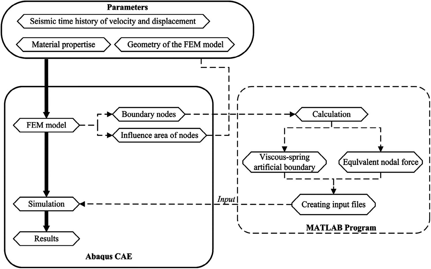
Figure 10: The flowchart of the implementation of viscous-spring artificial boundary and equivalent nodal force

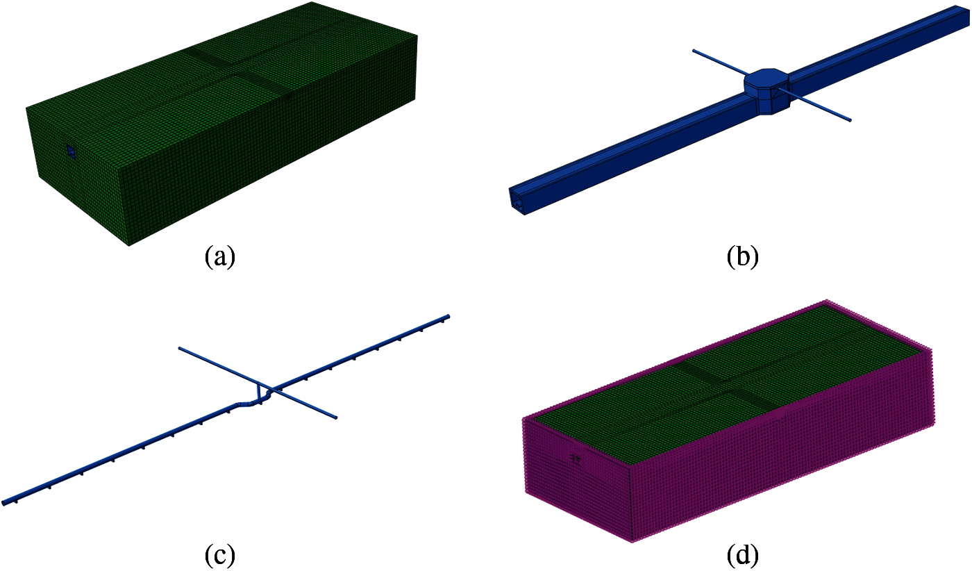
Figure 11: Finite element model (a) Soil model (b) Tunnel model (c) Pipe model (d) Viscous-spring boundary

4  Selection of Ground Motions

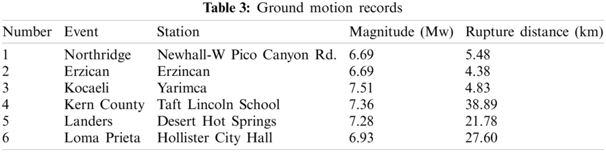
There have been 32 destructive earthquakes in Nanjing and its surrounding areas, recorded in history. These areas are likely to encounter near-fault earthquakes of magnitude over 6.0 and far-field earthquakes of magnitude 7.0–7.5 [37]. The fault distance of 20 km was taken as the limit in this paper [38], and three near-fault ground motions along with three far-field ground motions were selected from the PEER database [39] for numerical simulation and comparative analysis according to the site conditions and the requirements for the number of ground motions in the Chinese standard [40].

The Northridge earthquake in 1994, the Erzincan earthquake in 1992, and the Kocaeli earthquake in 1999 were selected as the excitations for near-fault ground motion. Similarly, the Taft earthquake in 1952, the Landers earthquake in 1992, and the Loma Prieta earthquake in 1989 were selected as the excitations for far-site ground motion, as shown in Table 3.

The mean acceleration response-spectrum values in the three directions are shown in Figs. 12a, 12c, 12e. To compare the difference of the response spectra between near-fault ground motion and far-field ground motion, they were normalized by adjusting the peak acceleration in the three directions of each group of ground motion to 1 m/s2, and the average acceleration response spectrum was drawn, as shown in Figs. 12b, 12d, 12f. In Fig. 12, the light solid line represents the three selected near-fault ground motions, and the dashed line represents the three selected far-field ground motions. When compared with the far-field ground motion, it was found that the near-fault ground motion had a stronger response over a long period, which was consistent with previous research [41].

In this paper, the amplitude of the ground-motion acceleration was adjusted. The horizontal ground motion was input according to the peak accelerations of 0.2 and 0.4 g, considering an earthquake intensity of VIII in the Chinese Code [42], and the vertical ground motion was adjusted to be 0.7 times the horizontal peak acceleration [43]. The values of 0.2 and 0.4 g represented the design and rare earthquakes, respectively. Considering the better seismic performance of the underground structure, this paper did not consider the 0.1 g condition, which represented a frequent earthquake. The duration of each ground motion was 15 s.

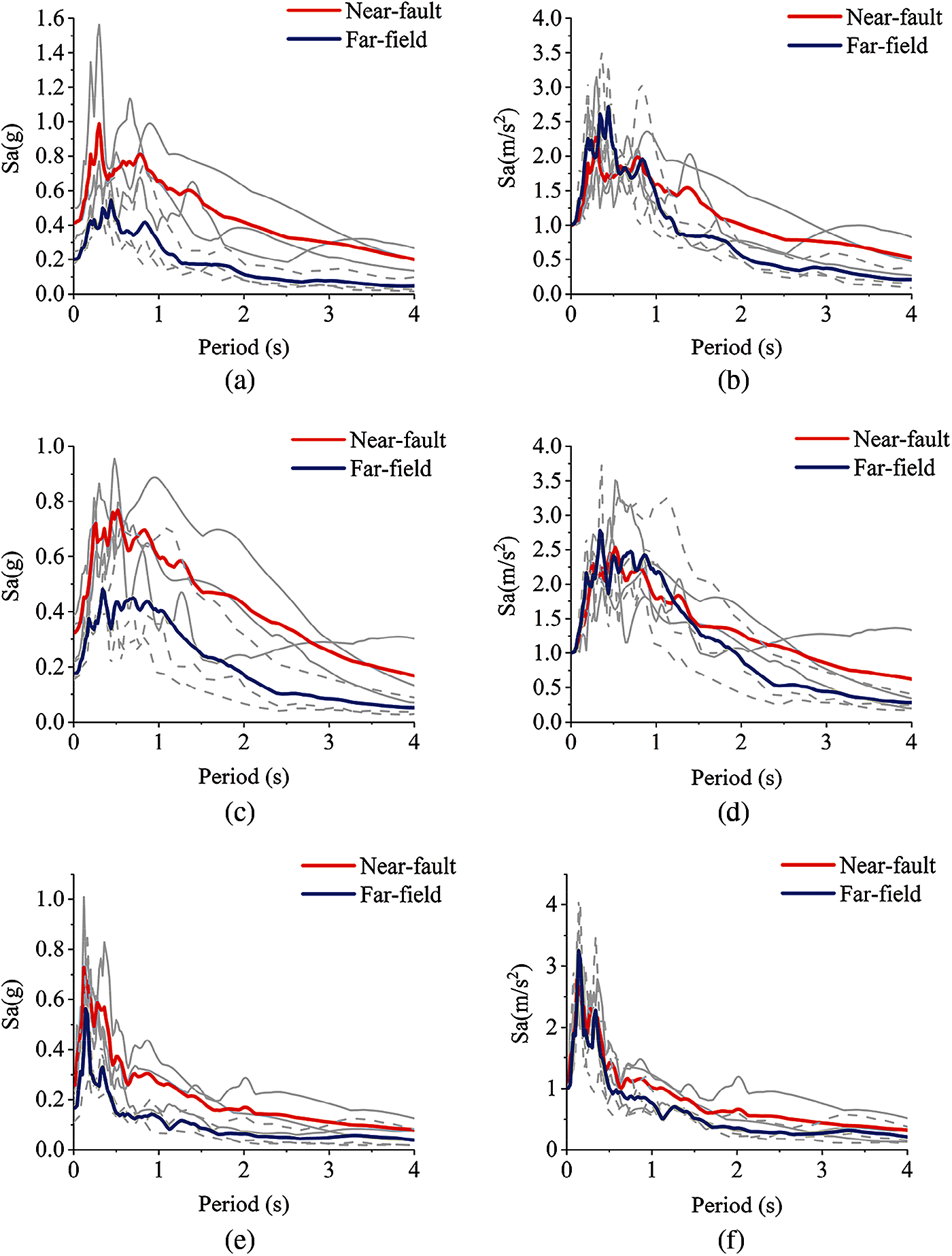
Figure 12: Ground-motion mean acceleration response-spectrum values (a) Mean response spectrum in the X-direction (b) Normalized mean response spectrum in the X-direction (c) Mean response spectrum in the Y-direction (d) Normalized mean response spectrum in the Y-direction (e) Mean response spectrum in the Z-direction (f) Normalized mean response spectrum in the Z-direction

5  Dynamic Response of Branch System

5.1 Damage Assessment of Tunnel

The results showed that the damage to the tunnel under a seismic intensity of 0.2 g was relatively light; so, only the damage to the tunnel under a seismic intensity of 0.4 g was counted. The locations of serious damage in the tunnel are shown in Fig. 13, which were concentrated in the connections between the standard segment, the branch joint A, and the branch-joint opening B. In this paper, the tunnel was mainly subjected to tensile damage; so, the damage variable mentioned below is a tensile-damage variable. Under bidirectional (X, Y) input and tridirectional (X, Y, Z) input of the ground motion, the number of elements with a damage variable greater than 0.5 [44] is shown in Fig. 14. It was found that far-field ground motions had little difference under bidirectional and tridirectional input conditions, but the number of damaged elements under the tridirectional input of near-fault ground motions was obviously more than that under bidirectional input and about 1.2 times greater than that of the bidirectional input. Considering that the number of elements in the branch joint only accounts for 30% of the total number of tunnel elements and most of the concrete that was unable to bear any more loading was concentrated near the branch joint, in fact, 1.2 times was a big increase. For far-field ground motions, the damage caused by the vertical component to the tunnel was very small. The reason for the small difference is the P-delta effect caused by the vertical component [45].

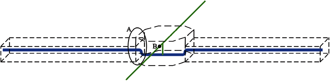
Figure 13: Diagram of tunnel damage location

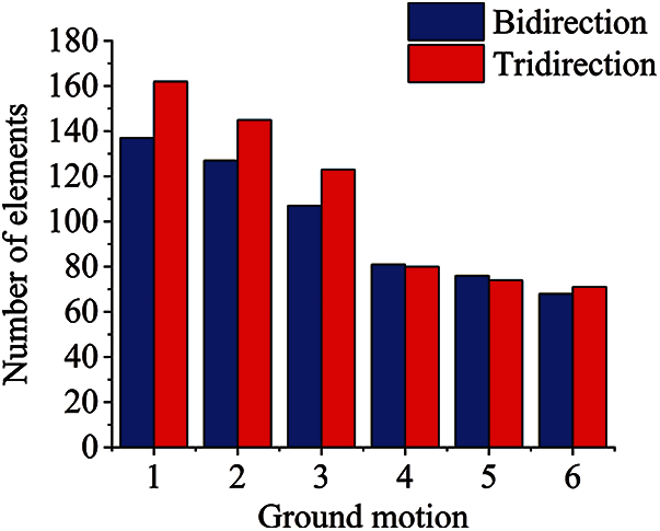
Figure 14: Number of damage elements

Taking Erzincan as an example, it was assumed that the elements with a damage variable greater than 0.5 failed to bear any load, and the red region shown in Fig. 15 represents the failed elements. Compared with the bidirectional-input condition, the tridirectional input directly led to the failure of elements on the roof of the connection between the standard segment and the branch joint, which could easily cause the tensile fracture of the tunnel. The tridirectional input also led to more serious damage at the opening of the branch joint, where the damage mainly occurred in the concrete casing but had little effect on the main structure of the surrounding tunnel.

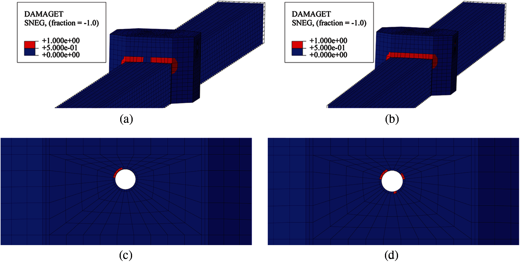
Figure 15: Tunnel damage under Erzincan 0.4 g seismic intensity (a) The connection of seismic bidirectional input (b) The connection of seismic tridirectional input (c) The opening of seismic bidirectional input (d) The opening of seismic tridirectional input

5.2 Stress Assessment of Pipe

Some representative sampling points were set on the pipe to extract the pipe stress, as shown in Fig. 16. Point A was the contact point between the pipe and the casing, point B was the buried pipe, point C was the overhead three-way pipe in the tunnel, point D was the fixed three-way pipe in the tunnel’s piers, point E was the curved pipe in the tunnel, and point F was the straight pipe in the tunnel.

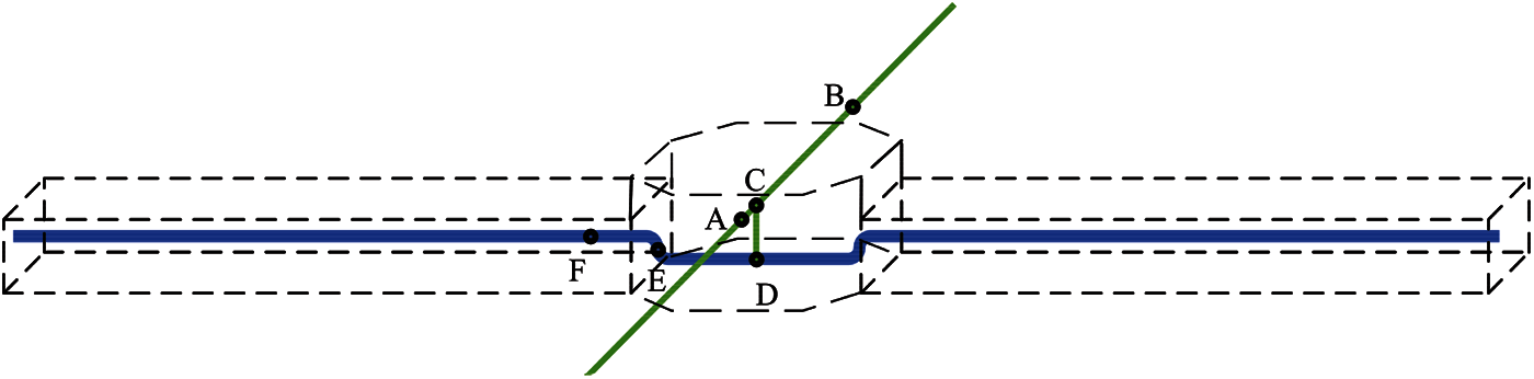
Figure 16: Pipe sampling points

The maximum stress of the pipeline sampling points under 0.4 and 0.2 g seismic intensities is shown in Figs. 17 and 18, respectively. There was only a slight difference between the pipe stress under bidirectional input and tridirectional input, which was different from the damage response of the tunnel; so, only the result of the tridirectional input is shown in Figs. 17 and 18.

Under 0.4 g seismic intensity, the near-fault seismic response (Fig. 17a) was significantly higher than the far-field seismic response (Fig. 17b), whereas under 0.2 g seismic intensity, the near-fault seismic response (Fig. 18a) was not significantly different from the far-field seismic response (Fig. 18b). A previous study [30] suggested that the pipe stress in the tunnel would be less than that of the general buried pipeline, but from this point of view, it was only true for the curved pipe E and straight pipe F in the tunnel. The stress level of the special joints such as contact point A, overhead three-way pipe C, and fixed three-way pipe D in the tunnel was significantly higher than that of other locations. In fact, for the pipes with a small elevation difference between the upper and lower three-way joints, the dislocation between the upper and lower pipes under the seismic action led to local joint stress concentrations easily.

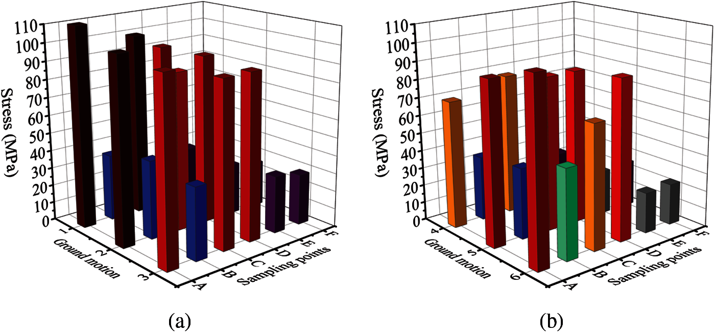
Figure 17: Maximum Mises stress of pipe under 0.4 g seismic intensity (a) Near-fault ground motions (b) Far-field ground motions

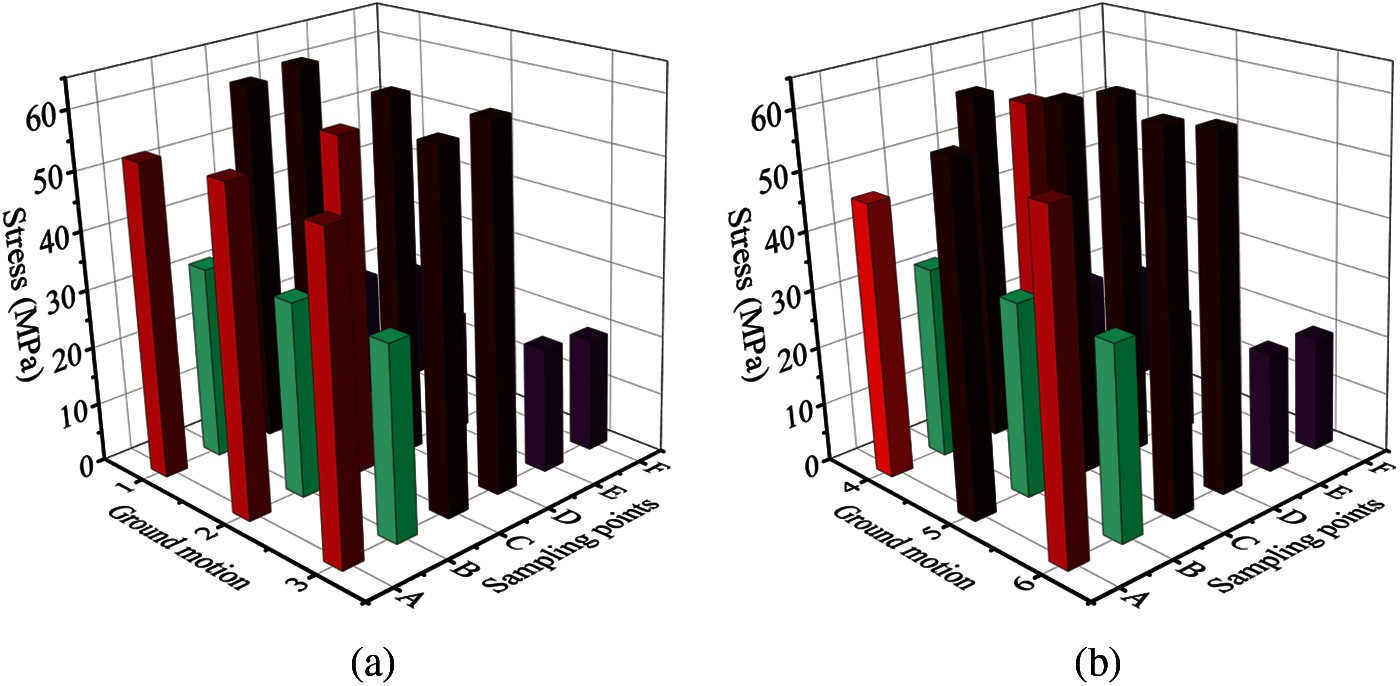
Figure 18: Maximum Mises stress of pipe under 0.2 g seismic intensity (a) Near-fault ground motions (b) Far-field ground motions

6  Conclusion

In this paper, the dynamic responses of the branch joint and inner pipelines of the urban-underground utility tunnel of Nanjing under near-fault and far-field earthquakes were studied according to bidirectional and tridirectional input. A viscous-spring artificial boundary was used to solve the semi-infinite space problem and simulate the energy dissipation. The equivalent nodal-force input method was deduced when a P wave and SV wave were incident vertically at the same time and was realized by the finite element method in ABAQUS software.

According to the dynamic-response results, near-fault and far-field earthquakes had significant influence on the structural response under different input mechanisms. The following conclusions were obtained:

1.    The influence of the vertical component of near-fault ground motion on the damage to the utility tunnel cannot be ignored, causing 20% more damaged elements in the tridirectional input than in the bidirectional input.

2.    The connection between the branch joint of the utility tunnel and the standard segment is the most seriously damaged part under an earthquake, which can easily cause tensile fracture under strong ground motion. Due to the existence of the concrete casing, the damage to the concrete main structure around the opening of the branch joint is very small.

3.    With the increase of the ground motion intensity, the pipe stress under the near-fault ground motion is significantly higher than that under far-field ground motion. For rare earthquakes, the pipe stress under a near-fault earthquake is 20%–50% higher than that under a far-field earthquake.

4.    The stress level of the straight or curved pipeline in the tunnel under ground motion is smaller than that of the general buried pipeline. However, for the dislocation between the special joints such as the three-way pipeline and the contact point between the pipe and the casing in the tunnel under ground motion, the stress level will rise sharply, being 2–3 times higher than the stress of the general pipe in the tunnel.

5.    In general, the branch system of the utility tunnel has as good a seismic performance as the traditional underground structure. Owing to its good mechanical properties, it can resist design earthquakes. Only the roof at the connection between the branch joint of the utility tunnel and the standard segment is damaged under a rare earthquake action, and the internal pipe stress does not reach the yield limit of the material.

Funding Statement: This research work was supported by National Key R&D Program of China under Grants No. 2019YFC1509301.

Conflicts of Interest: The authors declare that they have no conflicts of interest to report regarding the present study.

References

 1.  Cui, J. Q., Broere, W., Lin, D. (2021). Underground space utilisation for urban renewal. Tunnelling and Underground Space Technology, 108(3), 103726. DOI 10.1016/j.tust.2020.103726. [Google Scholar] [CrossRef]

 2.  Wang, H. D., Xue, W. C. (2013). Theory and practice of utility tunnel engineering. Beijing: China Architecture & Building Press (in Chinese). [Google Scholar]

 3.  Bai, Y. P., Zhou, R., Wu, J. S. (2020). Hazard identification and analysis of urban utility tunnels in China. Tunnelling and Underground Space Technology, 106, 103584. DOI 10.1016/j.tust.2020.103584. [Google Scholar] [CrossRef]

 4.  Tsunami Digital Library (2003) (in Japanese). http://tsunami-dl.jp/document/145. [Google Scholar]

 5.  Guo, J. Q., Qian, Y., Wang, Z. Z., Dun, Z. L., Liu, X. (2019). The common operational disasters and countermeasures of utility tunnel in urban. Journal of Catastrophology, 34(1), 27–33. [Google Scholar]

 6.  Federal Emergency Management Agency (1996). USGS response to an urban earthquake, Northridge '94. Washington: FEMA Press. [Google Scholar]

 7.  Liu, J. B., Wang, D. Y., Tan, H., Li, S. T., Bao, X. (2019). Theorectical derivation and consistency proof of the integral response deformation method. China Civil Engineering Journal, 52(8), 18–23. [Google Scholar]

 8.  Liu, J. B., Wang, W. H., Zhao, D. D., Zhang, X. B. (2013). Integral response deformation method for seismic analysis of underground structure. Chinese Journal of Rock Mechanics & Engineering, 32(8), 1618–1624. [Google Scholar]

 9.  Sun, W. W., Min, H. P., Chen, J. Z., Ruan, C., Zhang, Y. J. et al. (2021). Numerical analysis of three-layer deep tunnel composite structure. Computer Modeling in Engineering & Sciences, 127(1), 223–239. DOI 10.32604/cmes.2021.015208. [Google Scholar] [CrossRef]

10. Zhang, S. R., Wang, G. H. (2013). Effects of near-fault and far-fault ground motions on nonlinear dynamic response and seismic damage of concrete gravity dams. Soil Dynamics and Earthquake Engineering, 53(12), 217–229. DOI 10.1016/j.soildyn.2013.07.014. [Google Scholar] [CrossRef]

11. Pang, Y. T., Wei, H., Zhong, J. (2021). Risk-based design and optimization of shape memory alloy restrained sliding bearings for highway bridges under near-fault ground motions. Engineering Structures, 241(6), 112421. DOI 10.1016/j.engstruct.2021.112421. [Google Scholar] [CrossRef]

12. Hu, Y., Jiang, L. Q., Ye, J. H., Zhang, X. S., Jiang, L. Z. (2021). Seismic responses and damage assessment of a mid-rise cold-formed steel building under far-fault and near-fault ground motions. Thin-Walled Structures, 163(6), 107690. DOI 10.1016/j.tws.2021.107690. [Google Scholar] [CrossRef]

13. Mei, X. C., Sheng, Q., Cui, Z. (2021). Effect of near-fault pulsed ground motions on seismic response and seismic performance to tunnel structures. Shock and Vibration, 2021, 1–18. [Google Scholar]

14. Yu, H. T., Wang, Q. (2021). Analytical solution for deep circular tunnels covered by an isolation coating layer subjected to far-field shear stresses. Tunnelling and Underground Space Technology, 115, 104026. DOI 10.1016/j.tust.2021.104026. [Google Scholar] [CrossRef]

15. Sun, B. B., Zhang, S. R., Deng, M. J., Wang, C. (2020). Inelastic dynamic response and fragility analysis of arched hydraulic tunnels under as-recorded far-fault and near-fault ground motions. Soil Dynamics and Earthquake Engineering, 132, 106070. DOI 10.1016/j.soildyn.2020.106070. [Google Scholar] [CrossRef]

16. Yang, Y. S., Yu, H. T., Yuan, Y., Sun, J. (2021). 1g Shaking table test of segmental tunnel in sand under near-fault motions. Tunnelling and Underground Space Technology, 115(3), 104080. DOI 10.1016/j.tust.2021.104080. [Google Scholar] [CrossRef]

17. Jiang, L. Z., Chen, J., Li, J. (2010). Seismic response of underground utility tunnels: Shaking table testing and FEM analysis. Earthquake Engineering and Engineering Vibration, 9(4), 555–567. DOI 10.1007/s11803-010-0037-x. [Google Scholar] [CrossRef]

18. Chen, J., Shi, X. J., Li, J. (2010). Shaking table test of utility tunnel under non-uniform earthquake wave excitation. Soil Dynamics and Earthquake Engineering, 30(11), 1400–1416. DOI 10.1016/j.soildyn.2010.06.014. [Google Scholar] [CrossRef]

19. Pan, Y., Yi, D. H., Wu, W. L., Bao, Y. L., Guo, R. (2020). Mechanical performance test and finite element analysis of prefabricated utility tunnel L-shaped joint. Structural Design of Tall and Special Buildings, 29, e1748. [Google Scholar]

20. Zhou, R., Fang, W. P., Wu, J. S. (2020). A risk assessment model of a sewer pipeline in an underground utility tunnel based on a Bayesian network. Tunnelling and Underground Space Technology, 103(3), 103473. DOI 10.1016/j.tust.2020.103473. [Google Scholar] [CrossRef]

21. Liu, W., Song, Z., Wang, Y. (2020). Seismic analysis of the connections of buried segmented pipes. Computer Modeling in Engineering and Sciences, 123(1), 257–282. DOI 10.32604/cmes.2020.07220. [Google Scholar] [CrossRef]

22. Guo, E. D., Wang, P. Y., Liu, S. H., Wang, X. J. (2018). Seismic response analysis of typical utility tunnel system. Earthquake Engineering and Engineering Vibration, 38(1), 124–141. [Google Scholar]

23. Wang, T. Y., Tan, L. X., Xie, S. Y., Ma, B. S. (2018). Development and applications of common utility tunnels in China. Tunnelling and Underground Space Technology, 76(3), 92–106. DOI 10.1016/j.tust.2018.03.006. [Google Scholar] [CrossRef]

24. Valdenebro, J. V., Gimena, F. N. (2018). Urban utility tunnels as a long-term solution for the sustainable revitalization of historic centres: The case study of Pamplona-Spain. Tunnelling and Underground Space Technology, 81(4), 228–236. DOI 10.1016/j.tust.2018.07.024. [Google Scholar] [CrossRef]

25. Luo, Y., Alaghbandrad, A., Genger, T. K., Hammad, A. (2020). History and recent development of multi-purpose utility tunnels. Tunnelling and Underground Space Technology, 103(1–2), 32. DOI 10.1016/j.tust.2020.103511. [Google Scholar] [CrossRef]

26. Gu, Y., Liu, J. B., Du, Y. X. (2007). 3D consistent viscous-spring artificial boundary and viscous-spring boundary element. Engineering Mechanics, 24, 31–37. [Google Scholar]

27. He, J. T., Ma, H. F., Chen, H. Q. (2012). Calculation of structures comprehensive response under static and dynamic loads considering foundation radiation damping. World Earthquake Engineering, 28, 79–83. [Google Scholar]

28. He, J. T., Ma, H. F., Zhang, B. Y., Chen, H. Q. (2010). Method and realization of seismic motion input of viscous-spring boundary. Journal of Hydraulic Engineering, 41, 960–969. [Google Scholar]

29. Liu, J. B., Lu, Y. D. (1998). A direct method for analysis of dynamic soil-structure interaction based on interface idea. Developments in Geotechnical Engineering, 83(3), 261–276. DOI 10.1016/S0165-1250(98)80018-7. [Google Scholar] [CrossRef]

30. Liu, W., Wu, Q. X. (2020). Comparison between the seismic performance of buried pipes and pipes in a utility tunnel. Computer Modeling in Engineering and Sciences, 123(2), 661–690. DOI 10.32604/cmes.2020.07764. [Google Scholar] [CrossRef]

31. Lee, J., Fenves, G. L. (1998). Plastic-damage model for cyclic loading of concrete structures. Journal of Engineering Mechanics, 124(8), 892–900. DOI 10.1061/(ASCE)0733-9399(1998)124:8(892). [Google Scholar] [CrossRef]

32. Lubliner, J., Oliver, J., Oller, S., Oñate, E. (1989). A plastic-damage model for concrete. International Journal of Solids and Structures, 25(3), 299–326. DOI 10.1016/0020-7683(89)90050-4. [Google Scholar] [CrossRef]

33. Ministry of Housing and Urban-Rural Development of the China (2015). GB50010-2010: Code for Seismic Design of Buildings (modified in 2015). Beijing: China Architecture & Building Press. [Google Scholar]

34. Zhao, J. F., Du, X. L., Han, Q., Li, Y. L. (2007). An approach to numerical simulation for external source wave motion. Engineering Mechanics, 24, 52–58. [Google Scholar]

35. Ministry of Housing and Urban-Rural Development of the China (2011). GB50007-2011: Code for design of building foundation. Beijing: China Architecture & Building Press. [Google Scholar]

36. Ministry of Housing and Urban-Rural Development of the China (2014). GB51019-2014: Code for design of pipe racks and pipe sleepers in chemical industry. Beijing: China Architecture & Building Press. [Google Scholar]

37. Chen, L., Chen, G. X., Li, L. M. (2010). Seismic response characteristics of the double-layer vertical Overlapping metro tunnels under near-field and far-field ground motions. China Railway Science, 31, 79–86. [Google Scholar]

38. Li, S., Xie, L. L. (2007). Progress and trend on near-field problems in civil engineering. Acta Seismologica Sinica, 29(1), 102–111. DOI 10.1007/s11589-007-0105-0. [Google Scholar] [CrossRef]

39. Pacific Earthquake Engineering Research Center (2013). PEER NGA-WEST2 Strong Motion Database. Berkeley: University of California. https://ngawest2.berkeley.edu/. [Google Scholar]

40. Ministry of Housing and Urban-Rural Development of the China (2018). GB/T 51336-2018: Standard for seismic design of underground structures. Beijing: China Architecture & Building Press. [Google Scholar]

41. Cui, Z., Sheng, Q., Leng, X. L. (2018). Effects of a controlling geological discontinuity on the seismic stability of an underground cavern subjected to near-fault ground motions. Bulletin of Engineering Geology and the Environment, 77(1), 265–282. DOI 10.1007/s10064-016-0936-9. [Google Scholar] [CrossRef]

42. Ministry of Housing and Urban-Rural Development of the China (2015). GB 50011-2015: Code for seismic design of buildings. Beijing: China Architecture & Building Press. [Google Scholar]

43. Ministry of Housing and Urban-Rural Development of the China (2014). GB 50909-2014: Code for seismic design of urban rail transit structures. Beijing: China Architecture & Building Press. [Google Scholar]

44. Zhao, W. S., Chen, W. Z. (2015). Effect of near-fault ground motions with long-period pulses on the tunnel. Journal of Vibroengineering, 17, 841–858. [Google Scholar]

45. Xu, Z. G., Du, X. L., Xu, C. S., Hao, H., Bi, K. M. et al. (2019). Numerical research on seismic response characteristics of shallow buried rectangular underground structure. Soil Dynamics and Earthquake Engineering, 116, 242–252. DOI 10.1016/j.soildyn.2018.10.030. [Google Scholar] [CrossRef]

This work is licensed under a Creative Commons Attribution 4.0 International License, which permits unrestricted use, distribution, and reproduction in any medium, provided the original work is properly cited.