| Computer Modeling in Engineering & Sciences |
DOI: 10.32604/cmes.2022.016621
ARTICLE
COVID-19 Detection via a 6-Layer Deep Convolutional Neural Network
School of Computer Science and Technology, Henan Polytechnic University, Jiaozuo, 454000, China
*Corresponding Author: Ji Han. Email: HanJi@home.hpu.edu.cn
Received: 12 March 2021; Accepted: 05 August 2021
Abstract: Many people around the world have lost their lives due to COVID-19. The symptoms of most COVID-19 patients are fever, tiredness and dry cough, and the disease can easily spread to those around them. If the infected people can be detected early, this will help local authorities control the speed of the virus, and the infected can also be treated in time. We proposed a six-layer convolutional neural network combined with max pooling, batch normalization and Adam algorithm to improve the detection effect of COVID-19 patients. In the 10-fold cross-validation methods, our method is superior to several state-of-the-art methods. In addition, we use Grad-CAM technology to realize heat map visualization to observe the process of model training and detection.
Keywords: COVID-19; deep learning; convolutional neural network; max pooling; batch normalization; Adam; Grad-CAM
COVID-19 is a disease that easily spreads among people. It originated from the severe acute respiratory syndrome coronavirus 2 (SARS-CoV-2) [1]. The spread of this disease includes human-to-human contact, or contact with polluted air, as well as respiratory droplets and feces [2]. Therefore, the authorities have adopted a series of measures, including wearing masks in public places, quarantining people entering the country from abroad, and reminding people of the country not to travel to high-risk areas [3].
Early detection of COVID-19 helps various departments to take preventive and control measures in advance to protect the safety of local residents. The most commonly used testing methods are real-time reverse transcription polymerase chain reaction (RT-PCR) and point-of-care (POC) methods [4]. POC can be used to detect genes encoding viral proteins in respiratory samples, and this method test takes less than an hour to get the result. POC can be used to detect genes encoding viral proteins in respiratory samples. This method only takes a few minutes to get the test results. However, the sensitivity of these two methods may not be sufficient to detect early infections caused by low virus concentrations.
Traditional artificial intelligence (AI) methods [5] may not work well on handling complicated image processing tasks [6]. Now, many researchers use deep learning (DL) methods to optimize the detection of certain diseases based on medical images. For example, Guo et al. [7] employed ResNet-18 to detect Thyroid Ultrasound Standard Plane images. Wu [8] chose to combine wavelet Renyi entropy with their proposed three-segment biogeography-based optimization. Ni et al. [9] proposed a deep learning approach (DPA) for COVID-19 detection. Wang [10] combined graph convolutional network (GCN) with convolutional neural network (CNN) using deep feature fusion method. Wang [11] proposed a novel CCSH network to detect COVID-19. There are many other successful applications of deep learning cases [12–14], which all prove the powerfulness of DL.
In addition, more and more researchers also use transfer learning. Transfer learning is suitable for situations where a large number of source data features in the training model are similar to a small number of target data features in the detection model, so it is not suitable for our experiments. In this paper, we collected CT images of COVID-19 and proposed a 6-layer convolutional neural network method to detect COVID-19. Max pooling proved to perform better than other traditional pooling methods. Batch normalization effectively improves the training speed of convolutional neural networks. Adam algorithm is better than other algorithms in terms of model training effect.
The remaining chapters of this paper are as follows. Section 2 introduces the collection of datasets and the characteristics of the datasets. Section 3 describes the various modules of the convolutional neural network. Section 4 introduces the model we built and analyzes the experimental results. In the last section, we made a summary of our experiments and results.
The image dataset was from [15]. In the experiment, Philips Ingenuity 64-line spiral CT machines were used to collect lung pictures. During the CT scan, keep the patient supine and breathe deeply back, which helps scan from the lung tip to the rib diaphragm angle.
The image slices we collected came from 142 COVID-19 patients and 142 healthy people. From the CT images of each subject, 1–4 slices were selected as experimental data, and the resolution rate of all images was 1,024 × 1,024. Table 1 shows the characteristic data of the collected objects. In Fig. 1, we can find that the lung biopsy samples of COVID-19 patients have obvious white lesions.
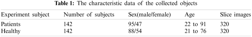
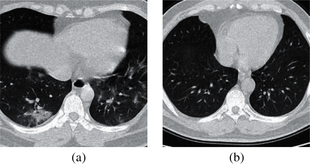
Figure 1: The sample of lung slices from patient with COVID-19 and healthy person. (a) COVID-19 (b) Normal
Convolutional neural network is a classifier, this method can identify normal images and abnormal images from medical images [16]. A classic neural network consists of an input layer, a convolutional layer, a pooling layer, a fully connected layer and an output layer [17,18]. The convolutional layer and the pooling layer are used to extract image features, and the fully connected layer is used for image classification. Fig. 2 shows the flowchart of CNN.
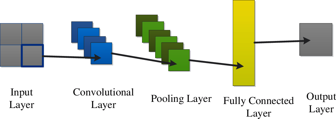
Figure 2: The flowchart of CNN
In the convolutional layer, the input image data and the kernel are convolved to output the feature map. The operation of the convolutional layer contains three hyperparameters [19], which are kernel size, filter depth, and stride. The kernel size represents the pixel size of the convolution filter. The filter depth controls the number of output feature maps, representing the number of filters in the convolutional layer. The stride determines how many pixels the filter will skip in each convolution [20]. The case of convolution operation is shown in Fig. 3. And the convolution operation is as follows:
where
Figure 3: The case of convolution operation
The convolutional layer will be followed by an activation function, such as Sigmoid and Relu, their activation curve is shown in Fig. 4. Sigmoid is a traditional non-linear activation function, and its output is bounded, and the output value ranges from 0 to 1 [21]. The activation formula is as follows:

Figure 4: The activation curve of Sigmoid and ReLU
Since the Sigmoid function encounters an input value that is too large or too small, its curve slope will tend to zero, which is likely to cause the gradient descent of the neural network. However, some of the output values of the ReLU function are 0, which avoids the problems existing in Sigmoid, which can reduce overfitting and solve the gradient descent problem. Therefore, compared with Sigmoid, the ReLU function can speed up model training. The calculation formula of Relu is as follows:
In the experiment, we used batch normalization technology [22] to solve the problem of internal covariate shift. This technology ensures that the data set distribution after convolution is more uniform, thereby increasing the learning rate of the training model and speeding up the training process [23]. The calculation steps for batch normalization are as follow. First, calculate the average of the minibatch
Second, calculate the variance of the minibatch
Third, in order to prevent abnormal operations, we added a constant
Finally, multiply
The pooling layer is used to reduce the dimensionality of the feature vector output after the convolution operation, which can prevent overfitting. The most common pooling methods are max pooling (Mp), average pooling (Ap) and

Figure 5: The three pooling operations
Suppose the pooling area is G, and the dataset to be activated in G is D. The definition of D is as follows:
The Mp was defined as
The Ap was defined as
The
3.5 Fully Connected Layer and Softmax
Fully connected layer (FCL) [25] is used to classify feature images after pooling [26]. And the neurons in the fully connected layer are fully connected to the neurons in the adjacent layer. The flowchart of the FCL is shown in Fig. 6. The calculation formula of the FCL is as follows:
where

Figure 6: The flowchart of the FCL
When the FCL is used for linear feature extraction, an activation function will follow. The most commonly used is the softmax activation function [28]. Its calculation formula is as follows:
Let
where
In the experiment, for the complexity of the deep learning training model, we chose a suitable optimization algorithm to optimize the model. Adam (Adaptive momentum) [29,30] is a gradient descent optimization technique that calculates the learning rate of each step by controlling the first and second moments of the gradient. And it can also correct the deviation and keep the parameters stable [31]. The formula for Adam is as follows:
where
In the experiment, we need to train and test the data set to verify the detection effect of the model. In order to analyze the performance of the constructed model, we adopted the cross-validation technology, which is a widely used method for optimizing and evaluating model performance [32,33].
We chose the K-fold cross-validation method to divide the collected data set into K equal subsets. K-1 equal subsets are trained in the experiment, and the one that is not trained is used for testing. This process is iterated k times, and each subset will be used for testing. In this paper, we used 10-fold cross validation, which has very little error in evaluating model performance. The operation of 10-fold cross validation is shown in Fig. 7.

Figure 7: The operation of 10-fold cross validation
In order to evaluate the performance of the built CNN model in training and testing the data set in the experiment, we selected some ideal indicators, including Sensitivity (
where
In the deep learning model, the entire training process cannot be visualized intuitively, so it is easy for radiologists to be confused whether the model can accurately detect abnormal areas in the CT image. We applied Grad-CAM technology to our model so that image features can be colored to easily distinguish between normal and abnormal regions in CT images [35]. Grad-CAM technology helps the model to accurately focus on key areas.
4 Experiment Results and Discussions
In the paper, we built a six-layer CNN. The architecture of the CNN is shown in Fig. 8. This CNN includes three convolutional layers, three max pooling layers and three FCLs. The parameters in the activation map are marked on each layer.

Figure 8: The architecture diagram of the 6-layer CNN
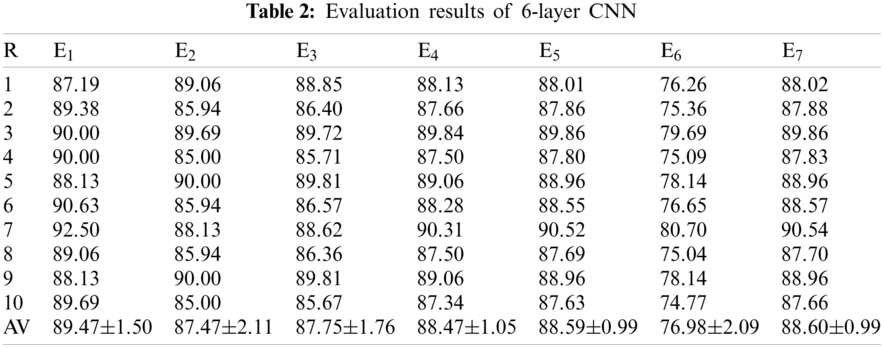
Table 2 shows the 7 evaluation index results of the 6-layer CNN we built under 10-fold cross-validation. The results of Sensitivity, Specificity, Precision, Accuracy, F1-Score, Matthews correlation coefficient, and Fowlkes Mallows index are 90.97%, 89.58%, 89.51%, 89.52%, 89.58%, 79.07%, and 89.59, respectively.
In the experiment, we applied the Mp layer to the six-layer CNN model, and compared with
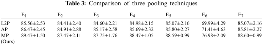

Figure 9: Comparison of three pooling techniques
4.4 Training Algorithm Comparison
In the experiment, we used Adam algorithm to optimize the 6-layer convolutional neural network and compared it with the SGDM and RMSProp optimization algorithms. SGDM is based on first-order momentum to reduce the oscillation in the best direction along the steepest path during the gradient descent process. RMSProp is an adaptive learning rate method that normalizes the gradient by using the exponential moving average of the gradient magnitude of each parameter. The experimental results are shown in Table 4 and Fig. 10. From the perspective of sensitivity (
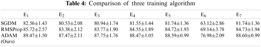

Figure 10: Comparison of three training algorithm
4.5 Comparison of Different Number of Conv Layers
When using CNN to detect CT images, increasing the number of convolutional layers is beneficial to improve the detection effect. But this does not mean that the more layers of convolutional layers, the better the result of the CNN. In order to select an appropriate number of convolutional layers, we compared the performance of convolutional neural networks with different convolutional layers in our experiments. The experimental results are shown in Table 5. We found that when the number of convolutional layers increased from 1 to 3, the performance became better and better, but when the number of layers continued to increase, the effect began to decrease. Therefore, our model works best when the number of convolutional layers is 3. At the same time, we made a clearer comparison in Fig. 11.
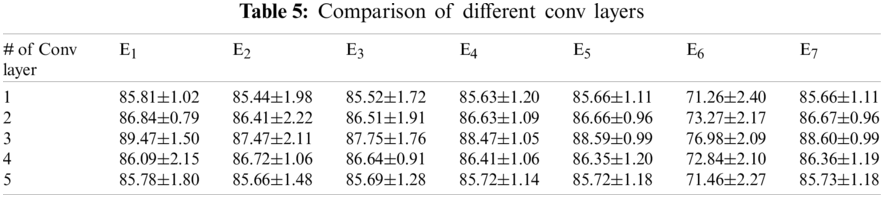

Figure 11: Comparison of different conv layers (conv lyers = CL)
4.6 Comparison of Different Number of FCLs
Most convolutional neural network models contain 2 fully connected layers, which can already achieve good results. But in our experiment, comparing the performance of models containing different numbers of FCLs, the experimental results are shown in Table 6, and Fig. 12 clearly shows their performance differences under various indicators. We found that when the number of FCLs in the model is 3, the performance is best.

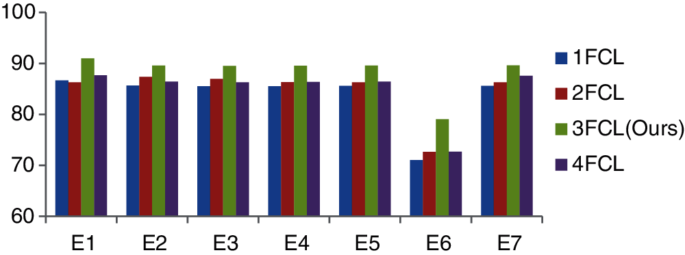
Figure 12: Comparison of different FCL layers
4.7 Comparison to State-of-the-Art Approaches
In the experiment, we compared our proposed method with several advanced methods, including ResNet-18 [7], WRE+ 3SBBO [8], and DPA [9]. Guo et al. [7]. proposed an 18-layer CNN model ResNet for image classification. Wu [8]. proposed a method based on a feedforward neural network and combining wavelet Renyi entropy and a proposed three-segment biogeography-based optimization (3SBBO) algorithm to detect COVID-19. Ni et al. [9]. used a deep learning method to accurately identify and quantitatively evaluate chest CT image features of patients with COVID-19. The comparison results based on 7 indicators are shown in Table 7, and the difference in the comparison results is clearly shown in Fig. 13. Although ResNet-18 [7] performs a little better on indicators
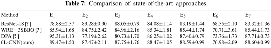

Figure 13: Comparison of state-of-the-art approaches
Fig. 14 shows the heatmap effect produced by using Grad-CAM technology to manipulate the image. Images b and d are heatmaps of the lung CT images of COVID-19 patients and healthy people, respectively. In Fig. 14b, the lung lesion area with COVID-19 is marked in red, while the healthy lung in Fig. 14d is not marked. It is found that the heatmap can clearly and accurately visualize the model detection area, which is beneficial to the guarantee of the model training process.

Figure 14: Heatmap of lungs of patients with COVID-19 and healthy people (a) COVID, (b) Heatmap of (a), (c) Healthy, (d) Heatmap of (c)
In this paper, we proposed a 6-layer CNN for the detection of COVID-19 and combined the Mp, batch normalization and Adam optimization algorithms. The effect of our proposed method is better than other state-of-the-art methods. The accuracy (E4) of our method reached 89.52%. Grad-CAM technology makes our models to be displayed more intuitively.
However, there is also a flaw in our research that the dataset is not very large, which will have little impact on the effect of model training. So, in future research, we will collect more data to ensure the adequacy of our proposed method in the training process. At the same time, we will build a more superior model based on DL methods to improve the result of COVID-19 detection. We will also share our methods so that other researchers can conduct research on our basis and accelerate the research speed of COVID-19 detection.
Funding Statement: The authors received no specific funding for this study.
Conflicts of Interest: The authors declare that they have no conflicts of interest to report regarding the present study.
1. Hotez, P. J., Fenwick, A., Molyneux, D. (2021). The new COVID-19 poor and the neglected tropical diseases resurgence. Infectious Diseases of Poverty, 10(1), 3. DOI 10.1186/s40249-020-00784-2. [Google Scholar] [CrossRef]
2. Patricio Silva, A. L., Prata, J. C., Walker, T. R., Duarte, A. C., Ouyang, W. et al. (2021). Increased plastic pollution due to COVID-19 pandemic: Challenges and recommendations. Chemical Engineering Journal, 405, 126683. DOI 10.1016/j.cej.2020.126683. [Google Scholar] [CrossRef]
3. Yildirim, M., Guler, A. (2021). Positivity explains how COVID-19 perceived risk increases death distress and reduces happiness. Personality and Individual Differences, 168, 110347. DOI 10.1016/j.paid.2020.110347. [Google Scholar] [CrossRef]
4. Giri, B., Pandey, S., Shrestha, R., Pokharel, K., Ligler, F. S. et al. (2020). Review of analytical performance of COVID-19 detection methods. Analytical and Bioanalytical Chemistry, 413(1), 35–48. DOI 10.1007/s00216-020-02889-x. [Google Scholar] [CrossRef]
5. Salehi, M., Farhadi, S., Moieni, A., Safaie, N., Hesami, M. (2021). A hybrid model based on general regression neural network and fruit fly optimization algorithm for forecasting and optimizing paclitaxel biosynthesis in Corylus avellana cell culture. Plant Methods, 17(1), 13. DOI 10.1186/s13007-021-00714-9. [Google Scholar] [CrossRef]
6. Reddy, B. S. N., Pramada, S. K., Roshni, T. (2021). Monthly surface runoff prediction using artificial intelligence: A study from a tropical climate river basin. Journal of Earth System Science, 130(1), 15. DOI 10.1007/s12040-020-01508-8. [Google Scholar] [CrossRef]
7. Guo, M., Du, Y. (2019). Classification of thyroid ultrasound standard plane images using ResNet-18 networks. 2019 IEEE 13th International Conference on Anti-counterfeiting, Security, and Identification, pp. 324–328. IEEE. [Google Scholar]
8. Wu, X. (2020). Diagnosis of COVID-19 by wavelet renyi entropy and three-segment biogeography-based optimization. International Journal of Computational Intelligence Systems, 13(1), 1332–1344. DOI 10.2991/ijcis.d.200828.001. [Google Scholar] [CrossRef]
9. Ni, Q., Sun, Z. Y., Qi, L., Chen, W., Yang, Y. et al. (2020). A deep learning approach to characterize 2019 coronavirus disease (COVID-19) pneumonia in chest CT images. European Radiology, 30(12), 6517–6527. DOI 10.1007/s00330-020-07044-9. [Google Scholar] [CrossRef]
10. Wang, S.-H. (2021). COVID-19 classification by FGCNet with deep feature fusion from graph convolutional network and convolutional neural network. Information Fusion, 67, 208–229. DOI 10.1016/j.inffus.2020.10.004. [Google Scholar] [CrossRef]
11. Wang, S. H. (2021). COVID-19 classification by CCSHNet with deep fusion using transfer learning and discriminant correlation analysis. Information Fusion, 68, 131–148. DOI 10.1016/j.inffus.2020.11.005. [Google Scholar] [CrossRef]
12. Alcaraz, J. C., Moghaddamnia, S., Peissig, J. (2021). Efficiency of deep neural networks for joint angle modeling in digital gait assessment. Eurasip Journal on Advances in Signal Processing, 2021(1), 20. DOI 10.1186/s13634-020-00715-1. [Google Scholar] [CrossRef]
13. Cabitza, F., Campagner, A., Sconfienza, L. M. (2021). Studying human-AI collaboration protocols: The case of the Kasparov's law in radiological double reading. Health Information Science and Systems, 9(1), 20. DOI 10.1007/s13755-021-00138-8. [Google Scholar] [CrossRef]
14. Santana, M. V. S., Silva, F. P. (2021). De novo design and bioactivity prediction of SARS-CoV-2 main protease inhibitors using recurrent neural network-based transfer learning. BMC Chemistry, 15(1), 20. DOI 10.1186/s13065-021-00737-2. [Google Scholar] [CrossRef]
15. Zhang, Y. D., Satapathy, S. C., Zhu, L. Y., Górriz, J. M., Wang, S. H. (2020). A seven-layer convolutional neural network for chest CT based COVID-19 diagnosis using stochastic pooling. IEEE Sensors Journal. DOI 10.1109/JSEN.2020.3025855. [Google Scholar] [CrossRef]
16. Panckow, R. P., McHardy, C., Rudolph, A., Muthig, M., Kostova, J. et al. (2021). Characterization of fast-growing foams in bottling processes by endoscopic imaging and convolutional neural networks. Journal of Food Engineering, 289, 12. DOI 10.1016/j.jfoodeng.2020.110151. [Google Scholar] [CrossRef]
17. Zhang, Y. D., Dong, Z. C. (2020). Advances in multimodal data fusion in neuroimaging: Overview, challenges, and novel orientation. Information Fusion, 64, 149–187. DOI 10.1016/j.inffus.2020.07.006. [Google Scholar] [CrossRef]
18. Wang, S. H., Zhang, Y. D. (2020). Densenet-201-based deep neural network with composite learning factor and precomputation for multiple sclerosis classification. ACM Transactions on Multimedia Computing, Communications, and Applications, 16(2s), 1–19. DOI 10.1145/3341095. [Google Scholar] [CrossRef]
19. Zunair, H., Ben Hamza, A. (2021). Synthesis of COVID-19 chest X-rays using unpaired image-to-image translation. Social Network Analysis and Mining, 11(1), 12. DOI 10.1007/s13278-021-00731-5. [Google Scholar] [CrossRef]
20. Park, E., Moon, Y. J., Shin, S., Yi, K., Lim, D. et al. (2018). Application of the deep convolutional neural network to the forecast of solar flare occurrence using full-disk solar magnetograms. The Astrophysical Journal, 869(2), 91. DOI 10.3847/1538-4357/aaed40. [Google Scholar] [CrossRef]
21. Sangaiah, A. K. (2020). Alcoholism identification via convolutional neural network based on parametric ReLU, dropout, and batch normalization. Neural Computing and Applications, 32, 665–680. DOI 10.1007/s00521-018-3924-0. [Google Scholar] [CrossRef]
22. Garbin, C., Zhu, X. Q., Marques, O. (2020). Dropout vs. batch normalization: An empirical study of their impact to deep learning. Multimedia Tools and Applications, 79(19–20), 12777–12815. DOI 10.1007/s11042-019-08453-9. [Google Scholar] [CrossRef]
23. Tiwari, S. (2021). Dermatoscopy using multi-layer perceptron, convolution neural network, and capsule network to differentiate malignant melanoma from benign nevus. International Journal of Cooperative Information Systems, 16(3), 58–73. DOI 10.4018/IJHISI.20210701.oa4. [Google Scholar] [CrossRef]
24. Zhang, Y. D., Satapathy, S. C., Liu, S., Li, G. R. (2021). A five-layer deep convolutional neural network with stochastic pooling for chest CT-based COVID-19 diagnosis. Machine Vision and Applications, 32(1), 1–13. [Google Scholar]
25. Assiri, A. S. (2021). Efficient training of multi-layer neural networks to achieve faster validation. Computer Systems Science and Engineering, 36(3), 435–450. DOI 10.32604/csse.2021.014894. [Google Scholar] [CrossRef]
26. Wang, S. H., Xie, S., Chen, X., Guttery, D. S., Tang, C. et al. (2019). Alcoholism identification based on an AlexNet transfer learning model. Frontiers in Psychiatry, 10, 205. DOI 10.3389/fpsyt.2019.00205. [Google Scholar] [CrossRef]
27. Urbaniak, I., Wolter, M. (2021). Quality assessment of compressed and resized medical images based on pattern recognition using a convolutional neural network. Communications in Nonlinear Science and Numerical Simulation, 95, 13. DOI 10.1016/j.cnsns.2020.105582. [Google Scholar] [CrossRef]
28. Huang, N., He, J., Zhu, N., Xuan, X., Liu, G. et al. (2018). Identification of the source camera of images based on convolutional neural network. Digital Investigation, 26, 72–80. DOI 10.1016/j.diin.2018.08.001. [Google Scholar] [CrossRef]
29. Loey, M., Manogaran, G., Taha, M. H. N., Khalifa, N. E. M. (2021). Fighting against COVID-19: A novel deep learning model based on YOLO-v2 with ResNet-50 for medical face mask detection. Sustainable Cities and Society, 65, 8. DOI 10.1016/j.scs.2020.102600. [Google Scholar] [CrossRef]
30. Benbahria, Z., Sebari, I., Hajji, H., Smiej, M. F. (2021). Intelligent mapping of irrigated areas from landsat 8 images using transfer learning. International Journal of Engineering Geosciences, 6(1), 41–51. DOI 10.26833/ijeg.681312. [Google Scholar] [CrossRef]
31. Mbah, T. J., Ye, H., Zhang, J., Long, M. (2021). Using LSTM and ARIMA to simulate and predict limestone price variations. Mining, Metallurgy & Exploration, 38(2), 913–926. DOI 10.1007/s42461-020-00362-y. [Google Scholar] [CrossRef]
32. Mutlu, A. Y., Yucel, O. (2018). An artificial intelligence based approach to predicting syngas composition for downdraft biomass gasification. Energy, 165, 895–901. DOI 10.1016/j.energy.2018.09.131. [Google Scholar] [CrossRef]
33. Nayak, D. R. (2017). Detection of unilateral hearing loss by stationary wavelet entropy. CNS & Neurological Disorders–Drug Targets, 16(2), 15–24. DOI 10.2174/1871527315666161026115046. [Google Scholar] [CrossRef]
34. Jena, R., Pradhan, B., Alamri, A. M. (2020). Susceptibility to seismic amplification and earthquake probability estimation using recurrent neural network (RNN) model in Odisha, India. Applied Sciences, 10(15), 5355. DOI 10.3390/app10155355. [Google Scholar] [CrossRef]
35. Panwar, H., Gupta, P. K., Siddiqui, M. K., Morales-Menendez, R., Bhardwaj, P. et al. (2020). A deep learning and grad-CAM based color visualization approach for fast detection of COVID-19 cases using chest X-ray and CT-scan images. Chaos, Solitons & Fractals, 140, 110190. DOI 10.1016/j.chaos.2020.110190. [Google Scholar] [CrossRef]
 | This work is licensed under a Creative Commons Attribution 4.0 International License, which permits unrestricted use, distribution, and reproduction in any medium, provided the original work is properly cited. |