| Computer Modeling in Engineering & Sciences |
DOI: 10.32604/cmes.2022.017257
ARTICLE
Performance Analysis of Magnetic Nanoparticles during Targeted Drug Delivery: Application of OHAM
1Institute of Energy and Environmental Engineering, University of the Punjab, Quaid-e-Azam Campus, Lahore, 54590, Pakistan
2Energy Research Centre, COMSATS University Islamabad, Lahore, 54000, Pakistan
3Department of Energy Engineering, Faculty of Mechanical and Aeronautical Engineering, University of Engineering and Technology, Taxila, 47080, Pakistan
4Department of Mathematics, COMSATS University Islamabad, Lahore, 54000, Pakistan
5School of Systems and Technology, University of Management Sciences and Technology, Lahore, 54770, Pakistan
6Department of Electrical, Electronics and Telecommunication Engineering, University of Engineering and Technology, Lahore (FSD Campus), Faisalabad, 38000, Pakistan
7Department of Electronic Engineering, Faculty of Applied Energy System, Jeju National University, Jeju Special Self-Governing Province, Jeju-si, 63243, Korea
*Corresponding Authors: Muhammad Zafar. Email: zaffarsher@gmail.com; Woo Young Kim. Email: semigumi@jejunu.ac.kr
#These authors contributed equally to this work
Received: 26 April 2021; Accepted: 03 August 2021
Abstract: In recent years, the emergence of nanotechnology experienced incredible development in the field of medical sciences. During the past decade, investigating the characteristics of nanoparticles during fluid flow has been one of the intriguing issues. Nanoparticle distribution and uniformity have emerged as substantial criteria in both medical and engineering applications. Adverse effects of chemotherapy on healthy tissues are known to be a significant concern during cancer therapy. A novel treatment method of magnetic drug targeting (MDT) has emerged as a promising topical cancer treatment along with some attractive advantages of improving efficacy, fewer side effects, and reduce drug dose. During magnetic drug targeting, the appropriate movement of nanoparticles (magnetic) as carriers is essential for the therapeutic process in the blood clot removal, infection treatment, and tumor cell treatment. In this study, we have numerically investigated the behavior of an unsteady blood flow infused with magnetic nanoparticles during MDT under the influence of a uniform external magnetic field in a micro-tube. An optimal homotopy asymptotic method (OHAM) is employed to compute the governing equation for unsteady electromagnetohydrodynamics flow. The influence of Hartmann number (Ha), particle mass parameter (G), particle concentration parameter (R), and electro-osmotic parameter (k) is investigated on the velocity of magnetic nanoparticles and blood flow. Results obtained show that the electro-osmotic parameter, along with Hartmann’s number, dramatically affects the velocity of magnetic nanoparticles, blood flow velocity, and flow rate. Moreover, results also reveal that at a higher Hartman number, homogeneity in nanoparticles distribution improved considerably. The particle concentration and mass parameters effectively influence the capturing effect on nanoparticles in the blood flow using a micro-tube for magnetic drug targeting. Lastly, investigation also indicates that the OHAM analysis is efficient and quick to handle the system of nonlinear equations.
Keywords: Hartmann number; magnetic nanoparticles; nonlinear analysis; targeted drug delivery; optimal homotopy asymptotic method (OHAM)
Nanotechnology is effectively playing its significant role in numerous fields such as structure, environment, molecular physics, chemistry, biology, material sciences, computer sciences, engineering, measurements, imaging, and many other disciplines of science and technology [1–6]. Likewise, the application of nanoparticles for drug delivery is also one of the critical forefronts of medical sciences. The use of nanoparticles or nanotubes, as detectors or biosensors, can be exploited as they suffer changes in their respective electrical properties upon application. Moreover, under the influence of the magnetic field, such particles can be called as magnetic nanoparticles.
Magnetic nanoparticles typically consist of nickel, cobalt, or iron and are clusters of magnetic particles where several individual particles are present. By the application of synthesized Fe3C, magnetic hyperthermia can be studied. Similarly, the intrinsic loss power value and a specific absorption rate can also be determined. It is a well-known fact that these aspects are much superior at lower magnetic nanoparticle concentrations [7].
Since blood can be considered a bio-magnetic fluid, prone to be affected upon the magnetic field’s application, the exploitation of magnetic fluid properties can help improve drug targeting through the transportation of magnetic particles in the blood [8]. The application of magnetic nanoparticles in biomedicine offer advantages of stability and size controllability of magnetic nanoparticles. The magnetic nanoparticle applications have been investigated in several diseases such as cardiovascular, endovascular, drug targeting, cancer tissues, and hyperthermia treatment for malignant tumor cells [9–11]. It has been investigated that the blood’s viscosity with magnetic particles caries from the blood under the magnetic field’s influence [12]. The magnetization of fluid under the magnetic field’s control, without the electric field’s induction, affects bio-magnetic fluid flow [12–15]. However, most of these studies did not account for the instability of blood flow [16]. Various mathematical models considered that the blood flow followed non-Newtonian fluid properties. The study of non-Newtonian blood flow characteristics in micro-tube under the magnetic field’s influence is carried out by Shaw et al. [17]. However, Bandyopadhyay et al. [18] studied the Newtonian model for investigating the blood flow through a constricted channel. More interestingly, Shit et al. [19] studied the pulsatile blood flow in an artery environment under the influence of magnetic dipole. Considering Newtonian fluid properties, various studies are conducted to investigate the transportation of magnetic nanoparticles, capture efficiency in a tube for targeted drug delivery, and the effect of nanoparticle augmentation [20–25]. The majority of these studies are focused on pressure gradient and electrokinetic force, which necessitated the further exploration of magnetic nanoparticles and blow, together, in a channel, under the influence of the magnetic field, electrokinetic force, and pressure gradient.
Recently, a semi-analytic approximate method emerged for handling time-dependent partial differential equations, known as the optimal homotopy asymptotic method (OHAM). Compared to numerical methods, the optimal homotopy asymptotic method (OHAM) is powerful and straightforward. It achieves outcomes more quickly while maintaining acceptable results and good agreement with numerical methods. This method combines the advantages of the homotopy principle with an efficacious computational algorithm that gives a thorough and straightforward approach for controlling solution convergence [26–28]. The main advantage of OHAM is that it is free of parameters, does not require identifying the
The present study provides insight into the movement of magnetic nanoparticles in a tube with blood flow under the collective effect of the electrokinetic force, magnetic field, and pulsatile pressure gradient. It is well-established that the ability to predict the capture of nanoparticles under the influence of a magnetic field in vivo is essential. In this study, we solved the governing equations to predict blood flow and magnetic particle velocity using the optimal homotopy asymptotic method approach. The parametric study is used here to compute the solutions for the non-dimensional velocity of magnetic particles and blood. These studies’ findings may further explore magnetic therapy viability with magnetic nanoparticles to help design medical devices and drug delivery systems for blood clot removal, infection treatment, and tumor cell treatment.
In the current study, a two-dimensional mathematical formulation based on an unsteady and incompressible blood flow together with magnetic nanoparticles in a cylindrical vessel under the presence of a uniform external magnetic field and an axial electric field is considered. The schematic illustration of the physical problem is presented in Fig. 1, where the

Figure 1: Schematic representation of the physical problem (Reproduced with permission from A. Mondal and G. C. Shit, Journal of Magnetism and Magnetic Materials; published by Elsevier B. V., 2017)
2.1.1 Distribution of Electrical Potential
For at any point
where
where
The overall charge density distribution can be given as the sum of all cations and anions in the solution, assuming the equilibrium Boltzmann distribution,
where
Accordingly, Eq. (2) can be rewritten as
where
Now, introducing a normalized electro-osmotic potential function
where
In terms of the non-dimensional variables described in Eqs. (5), (7) gives
where
The electric potential distribution solution from the Eq. (8) by Eq. (9) can be given in the form of the modified Bessel function of the first kind as
where
The flow of blood together with the magnetic nanoparticle velocity inside a micro-vessel (assuming cylindrical polar coordinates) is expressed by the governing equation of electron magnetohydrodynamic [22,34,35]
We assumed that a spherical magnetic nanoparticle motion in a viscous carrier fluid is governed by the applied magnetic and electric field effect. The viscous drag and magnetic forces during slow motion are responsible forces, and thus ignoring the Brownian motion, the movement of the nanoparticles is given by the second law of motion (Newton’s) [35–38].
where
If the mass of a particle is likely to be negligible, the inertia term
By using Stoke’s law for the drag on a sphere, the fluidic force encountered by a particle (considering low Reynolds number) is estimated by
If the force acting on the particle is fluidic in one dimension [22,36], i.e.,
Along the axial direction the pulsatile pressure gradient can be given as [18]
where
The boundary conditions for magnetic nanoparticles and fluid velocity can be put mathematically in the form of
The following non-dimensional variables can be introduced as
with
and non-dimensional boundary conditions take the following form:
where
The dimensionless mathematical expression for the wall shear stress (WSS)
The optimal homotopy analysis method for the equation is as follows [40]:
with boundary conditions
This section describes the OHAM principle, and the following differential equation can be used to demonstrate the basic concept of the OHAM.
It depends on the following boundary condition:
where
First of all, build a series of equations using the OHAM [41,42]
with the boundary condition
where
Accordingly, as
The auxiliary function can be considered now, which can be expressed in the following way:
where
In the following way, expanding
A series of differential equations with boundary conditions are derived by putting Eq. (28) into Eq. (24), gathering the same power of
The following expression for residual is obtained by substituting Eq. (29) in Eq. (23)
If
The constants
These constants are used to determine the approximate solution (of order m) from Eq. (29).
This section describes the OHAM application to the differential Eq. (3). Moreover, we can build homotopy of the Eq. (3) according to the OHAM [39] as follows:
Considering
then putting the value of
with the conditions
we get from Eq. (35)
and similarly with the conditions
we get
Now for
we get
Hence the value of
By the method of least squares, the expression for residual becomes
Herewith
The values of constants
which give the following values of constants
Assuming the values of
Now for the Eqs. (18) and (19) with boundary conditions
with boundary conditions
with
and
According to OHAM for Eq. (42)
Now the formulation of OHAM for Eq. (43)
with the conditions
we get from Eq. (44)
now with the conditions
we get from Eq. (45)
for
we get from Eq. (46)
now the equation
Becomes
Now using the relationship
we get
Again using the relationship
gives
Similarly with
we get
Now with the equation
gives
The residue term for the function
Now from Eq. (31), the value is taken. And, the function
The description of the process for the initial guess required to initiate the OHAM process is given in detail somewhere else [31–33].
2.1.6 Non-Dimensional Velocity of the Blood
Using the least square method
and with the setting
various values of
Now with
The values of


The values of

Now change
The values of
2.1.7 Non-Dimensional Velocity of the Magnetic Particles
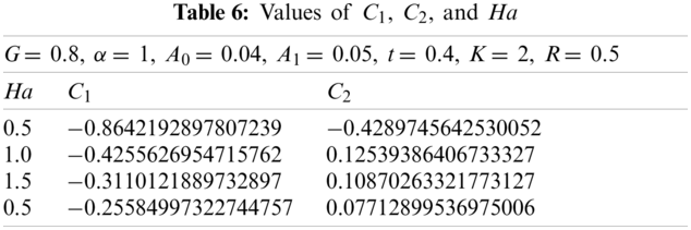
Here with G = 0.2, α = 1, A0 = 0.04, A1 = 0.05, t = 0.4, k = 2, and R = 0.5. Using the similar technique as earlier, the obtained values of

The values of
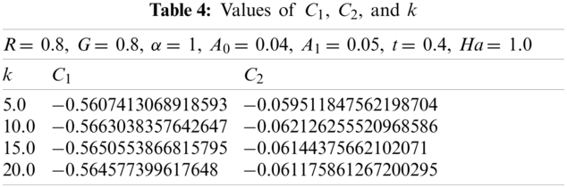
Here with G = 0.8, α = 1, A0 = 0.04, A1= 0.05, t = 0.4, k = 2, and R = 0.5. Using the similar technique as earlier, the obtained values of
The values of
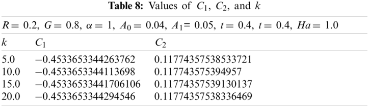
Now with G = 0.2, α = 1, t = 0.4, A0 = 0.04, A1 = 0.05, Ha = 1.0, and R = 0.2. Using the similar technique as earlier, for various values of k, the obtained values of

Now with G = 0.8, α = 1, t = 0.4, A0= 0.04, A1= 0.05, Ha = 1.0, and R = 0.2. Using the similar procedure as earlier, for various values of k, the following values of
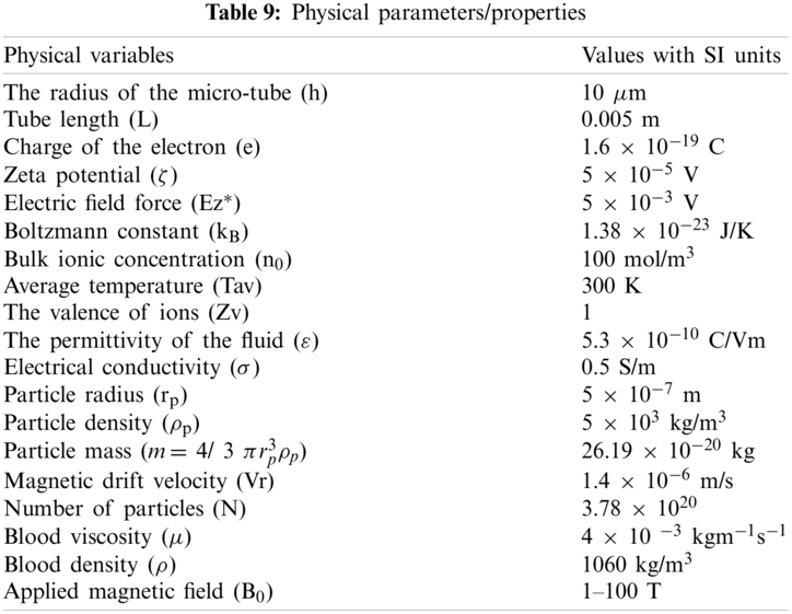
Values of various physical parameters and properties used during this study are given in Table 9.
3.1 Non-Dimensional Velocity of the Blood as a Function of Ha at G = 0.2
In Fig. 2, the Hartmann number (Ha) influence was studied at four different values; however, the particle mass parameter (G) was 0.2. The non-dimensional velocity (u) of the blood varied at various values of Ha, but at the end, velocity converged at r = 1.

Figure 2: Non-dimensional velocity of the blood as a function of Ha at G = 0.2
3.2 Non-Dimensional Velocity of the Blood as a Function of Ha at G = 0.8
In Fig. 3, the Hartmann number (Ha) effect was studied at four different values; however, the particle mass parameter (G) was kept at 0.8. Figs. 2 and 3 showed a similar trend despite increasing G, i.e., 0.8. Fig. 2 described the influence of Ha on the non-dimensional velocity of the blood. The blood’s non-dimensional velocity varied at various values of Ha, but in the end, velocity converged at r = 1.

Figure 3: Non-dimensional velocity of the blood as a function of Ha at G = 0.8
3.3 Non-Dimensional Velocity of the Blood as a Function of k at R = 0.2
In Fig. 4, the effect of an electro-osmotic parameter (k) was studied at four different values; however, the particle concentration parameter (R) was kept at 0.2. Fig. 4 trend was sinusoidal except at the curve where k = 5. The figure described the effect of varying k (from 5 to 20 with increments of 5) on the non-dimensional velocity of the blood. The non-dimensional velocity of blood changed as sinusoidal at four various values of k, but in the end, velocity converged at r = 1. It can be seen that the velocity declined as k rises until r = 0.3, and the final solution converged at r = 0.3. Hereafter, the velocity once more dropped then rises up to r = 0.8, where the curves converged, rose over with the last drop, and ultimately converged at r = 1.

Figure 4: Non-dimensional velocity of the blood as a function of k at R = 0.2
3.4 Non-Dimensional Velocity of the Blood as a Function of k at R = 0.8
In Fig. 5, the effect of an electro-osmotic parameter (k) was studied at four different values; however, the particle concentration parameter (R) was kept constant at 0.8. Fig. 5 trend was sinusoidal except at the curve where k = 5. The figure described the effect of varying k (from 5 to 20 with increments of 5) on the non-dimensional velocity of the blood. The non-dimensional velocity of blood changed as sinusoidal at four various values of k, but in the end, velocity converged at r = 1. It can be seen that the velocity declined as K rises until r = 0.3, and the final solution converged at r = 0.3. Hereafter, the velocity once more dropped then rises up to r = 0.8, where the curves converged, rose over with the last drop, and ultimately converged at r = 1.

Figure 5: Non-dimensional velocity of the blood as a function of k at R = 0.8
3.5 Non-Dimensional Velocity of the Magnetic Particles as a Function of Ha at G = 0.2
In Fig. 6, the Hartmann Number effect was studied at four different values; however, the particle mass parameter (G) was kept constant at 0.2. The magnetic particle’s velocity (v) varied at four various Ha values, but in the end, velocity converged at r = 1. The velocity of magnetic particles declined as the Hartmann number increased from 0.5 to 2.0 (with increments of 0.5).

Figure 6: Non-dimensional velocity of the magnetic particles as a function of Ha at G = 0.2
3.6 Non-Dimensional Velocity of the Magnetic Particles as a Function of Ha at G = 0.8
In Fig. 7, the Hartmann Number effect was studied at four different values; however, the particle mass parameter (G) was kept constant at 0.8. The magnetic particle’s velocity (v) varied at four various Ha values, but in the end, velocity converged at r = 1. The velocity of magnetic particles declined as the Hartmann number increased from 0.5 to 2.0 (with increments of 0.5).

Figure 7: Non-dimensional velocity of the magnetic particles as a function of Ha at G = 0.8
3.7 Non-Dimensional Velocity of the Magnetic Particles as a Function of k at R = 0.2
In Fig. 8, the effect of an electro-osmotic parameter (k) was studied at four different values; however, the particle concentration parameter (R) was kept at 0.2. Fig. 8 trend was sinusoidal except at the curve where k = 5. The figure described the effect of varying k (from 5 to 20 with increments of 5) on the magnetic particles’ velocity.

Figure 8: Non-dimensional velocity of the magnetic particles as a function of k at G = 0.2
3.8 Non-Dimensional Velocity of the Magnetic Particles as a Function of k at R = 0.8
In Fig. 9, the effect of an electro-osmotic parameter (k) was studied at four different values; however, the particle concentration parameter (R) was kept constant at 0.8. Fig. 9 trend was sinusoidal except at the curve where k = 5. The figure described the effect of varying k (from 5 to 20 with increments of 5) on the magnetic particles’ non-dimensional velocity. The magnetic particles' non-dimensional velocity changed as sinusoidal at four various values of k, but in the end, velocity converged at r = 1. It can be seen that the velocity declined as k rises until r = 0.3, and the final solution converged at r = 0.3. Hereafter, the velocity once more dropped then rises up to r = 0.8, where the curves converged, rose over with the last drop, and ultimately converged at r = 1.

Figure 9: Non-dimensional velocity of the magnetic particles as a function of k at G = 0.8
3.9 Non-Dimensional Velocity of the Blood
The particle mass parameter (G) was chosen as 0.2 or 0.8. The non-dimensional velocity of blood decreased as the Hartmann number increases, i.e., Ha = 0.0 to 1.5 (with increments of 0.5). The declining value of velocity was owing to two factors specifically: electrical conductivity (σ) and radius of micro-tube (h). When h increased, the Ha also increased, thus increasing Ha led to a decrease in the value of velocity, the non-dimensional velocity of the blood. The existence of a Lorentz resistive force opposes the flow of blood during the interaction with a magnetic field, which results in a decline in velocity of the blood with augment in Ha.
When h increased, σ also increased due to the presence of EDL at the boundary of the micro-tube, so eventually, velocity also increased. Changing the value of G from 0.2 to 0.8, all the effects were the same as discussed above. It can be seen in Figs. 2 and 3.
Selecting particle concentration parameter (R) as 0.2 or 0.8 and changing the value of electro-osmotic parameter, i.e., k = 5 to 20 (with increments of 5), the non-dimensional velocity of the blood exhibited sinusoidal behavior. This sinusoidal behavior was due to the radical relationship of Debye length (EDL thickness). The presence of EDL at the micro-tube circumference gave an increase to a higher bulk ionic concentration (
3.10 Non-Dimensional Velocity of the Magnetic Particles
Choosing particle mass parameter (G) as 0.2 or 0.8, the non-dimensional velocity of blood decreased as Hartmann number rises, i.e., Ha = 0.0 to 1.5 (with increments of 0.5). The declining value of velocity resulted from two factors: electrical conductivity (σ) and micro-tube radius (h). When h increased, the Ha also increased, so increasing Ha decreased the non-dimensional velocity of magnetic particles. This is most likely due to increasing the strength of the magnetic field in the micro-tube. Furthermore, as the particle mass parameter (G) is increased, the particle velocity decreases. This decline in the velocity is most probably as a result of the aggregation of the magnetic particles. When h increased, σ also increased due to EDL at the micro-tube boundary, so ultimately, velocity also increased. It can be seen in Figs. 6 and 7.
Selecting particle concentration parameter (R) as 0.2 or 0.8 and changing the value of an electro-osmotic parameter, i.e., k = 5 to 20 (with increments of 5), the non-dimensional velocity of magnetic particles showed sinusoidal behavior. The magnetic particle’s velocity varied as sinusoidal at four various Ha values, but in the end, velocity converged at r = 1. This sinusoidal behavior was due to the radical relationship of Debye length (EDL thickness). The presence of EDL at the micro-tube circumference contributed to a higher bulk ionic concentration (
To validate the computational results of the current study, the calculated blood velocity from this study has been compared with the Crank-Nicolson method computing the characteristic of blood flow [16]. Table 10 presents the comparison of OHAM calculated results with the Crank-Nicolson values for the blood flow. The OHAM computed the parametric conditions precisely by giving a similar trend along the radius of the micro-tube, as shown in Table 10. It can be seen that OHAM results are in accordance with the Crank-Nicolson results for the blood flow. These computed results demonstrate that the OHAM performs satisfactorily and is valid. Accordingly, the OHAM approach can be used to predict the performance of magnetic drug targeting.

The present investigation focuses on a theoretical analysis of the blood flow and moment of magnetic nanoparticles inside a cylindrical micro-tube under the influence of both a magnetic field and an electric potential. The Debye-Hückel approximation is used to determine the electro-osmotically steered capillary dynamics of blood inside a micro-tube. In this study, we found that the non-dimensional velocity of magnetic particles and non-dimensional velocity of blood may depend upon various constants and parameters like electro-osmotic parameter (k), particle concentration parameter (R), particle mass parameter (G), and Hartmann number (Ha). Using the OHAM approach, the dimensionless form of governing equations was numerically computed and showed rapid convergence. Maximum velocity of magnetic particles is achieved along the center of the micro-tube. The moment of the magnetic particles can be controlled by altering the strength of the axially applied electric field as well as the magnetic field. In order to validate our computed results, we compared them with the relevant data, which revealed reasonable agreement. From this study, we can deduce that the flow of blood and magnetic particles can be substantially enhanced by adjusting the magnitudes of the transverse electric field and the applied magnetic field. It may be deduced that the presence of magnetic nanoparticles in blood fluids could be beneficial in therapeutic solicitations, especially in the case of drug delivery. This analysis of nanofluids reflects the escalation findings in thermal levels by accumulating additional nanoparticles to the primary liquids. It was found that by the levels by accumulating different nanoparticles, the capacity of thermal conduction of the base liquid intensified. Such investigation was also established for the magnetic nanoparticles, as indicated in the results. The greater and intensifying effect of nanoparticles may lead to better drug delivery.
Acknowledgement: The authors would like to acknowledge the University of the Punjab and COMSATS University, Pakistan, for providing the necessary assistance to carry out this research work. The authors are also grateful to Dr. Arif Masud from the University of Illinois, Urbana-Champaign, the United States of America, who provided us with valuable direction during this research work. Furthermore, we would like to appreciate the Super Computing facility at Ghulam Ishaq Khan Institute of Engineering Sciences and Technology, Khyber Pakhtunkhwa, Pakistan.
Funding Statement: This work was supported by the research grant of Jeju National University in 2020, the Basic Science Research Program through the National Research Foundation of Korea (NRF) grant funded by the Korea Government (Ministry of Science and ICT) (NRF-2018R1A4A1025998), and Higher Education Commission of Pakistan (Project No. 210-3800/NRPU/R&D/HEC/1530).
Conflicts of Interest: The authors declare that they have no conflicts of interest to report regarding the present study.
1. Emerich, D. F., Thanos, C. G. (2003). Nanotechnology and medicine. Expert Opinion on Biological Therapy, 3(4), 655–663. DOI 10.1517/14712598.3.4.655. [Google Scholar] [CrossRef]
2. Chen, J. R., Miao, Y. Q., He, N. Y., Wu, X. H., Li, S. J. (2004). Nanotechnology and biosensors. Biotechnology Advances, 22(7), 505–518. DOI 10.1016/j.biotechadv.2004.03.004. [Google Scholar] [CrossRef]
3. Weiss, J., Takhistov, P., McClements, D. J. (2006). Functional materials in food nanotechnology. Journal of Food Science, 71(9), 107–116. DOI 10.1111/j.1750-3841.2006.00195.x. [Google Scholar] [CrossRef]
4. Paul, D. R., Robeson, L. M. (2008). Polymer nanotechnology: Nanocomposites. Polymer, 49(15), 3187–3204. DOI 10.1016/j.polymer.2008.04.017. [Google Scholar] [CrossRef]
5. DeRosa, M. C., Monreal, C., Schnitzer, M., Walsh, R., Sultan, Y. (2010). Nanotechnology in fertilizers. Nature Nanotechnology, 5(2), 91. DOI 10.1038/nnano.2010.2. [Google Scholar] [CrossRef]
6. Sanchez, F., Sobolev, K. (2010). Nanotechnology in concrete–A review. Construction and Building Materials, 24(11), 2060–2071. DOI 10.1016/j.conbuildmat.2010.03.014. [Google Scholar] [CrossRef]
7. Bartoszek, M., Drzazga, Z. (1999). A study of magnetic anisotropy of blood cells. Journal of Magnetism and Magnetic Materials, 196, 573–575. DOI 10.1016/S0304-8853(98)00838-5. [Google Scholar] [CrossRef]
8. Lübbe, A. S., Alexiou, C., Bergemann, C. (2001). Clinical applications of magnetic drug targeting. Journal of Surgical Research, 95(2), 200–206. DOI 10.1006/jsre.2000.6030. [Google Scholar] [CrossRef]
9. Alexiou, C., Schmidt, A., Klein, R., Hulin, P., Bergemann, C. et al. (2002). Magnetic drug targeting: Biodistribution and dependency on magnetic field strength. Journal of Magnetism and Magnetic Materials, 252, 363–366. DOI 10.1016/S0304-8853(02)00605-4. [Google Scholar] [CrossRef]
10. Ghasemi, S. E., Hatami, M., Sarokolaie, A. K., Ganji, D. D. (2015). Study on blood flow containing nanoparticles through porous arteries in presence of magnetic field using analytical methods. Physica E: Low-Dimensional Systems and Nanostructures, 70(4), 146–156. DOI 10.1016/j.physe.2015.03.002. [Google Scholar] [CrossRef]
11. Ghasemi, S. E. (2017). Thermophoresis and Brownian motion effects on peristaltic nanofluid flow for drug delivery applications. Journal of Molecular Liquids, 238(11), 115–121. DOI 10.1016/j.molliq.2017.04.067. [Google Scholar] [CrossRef]
12. Haik, Y., Pai, V., Chen, C. J. (2001). Apparent viscosity of human blood in a high static magnetic field. Journal of Magnetism and Magnetic Materials, 225(1–2), 180–186. DOI 10.1016/S0304-8853(00)01249-X. [Google Scholar] [CrossRef]
13. Kingsley, J. D., Dou, H., Morehead, J., Rabinow, B., Gendelman, H. E. et al. (2006). Nanotechnology: A focus on nanoparticles as a drug delivery system. Journal of Neuroimmune Pharmacology, 1(3), 340–350. DOI 10.1007/s11481-006-9032-4. [Google Scholar] [CrossRef]
14. Shyy, W., Narayanan, R. (1999). Fluid dynamics at interfaces. Cambridge, UK: Cambridge University Press. [Google Scholar]
15. Misra, J. C., Shit, G. C. (2009). Biomagnetic viscoelastic fluid flow over a stretching sheet. Applied Mathematics and Computation, 210(2), 350–361. DOI 10.1016/j.amc.2008.12.088. [Google Scholar] [CrossRef]
16. Mondal, A., Shit, G. C. (2017). Transport of magneto-nanoparticles during electro-osmotic flow in a micro-tube in the presence of magnetic field for drug delivery application. Journal of Magnetism and Magnetic Materials, 442(9), 319–328. DOI 10.1016/j.jmmm.2017.06.131. [Google Scholar] [CrossRef]
17. Shaw, S., Murthy, P. V. S. N., Pradhan, S. C. (2010). Effect of non-Newtonian characteristics of blood on magnetic targeting in the impermeable micro-vessel. Journal of Magnetism and Magnetic Materials, 322(8), 1037–1043. DOI 10.1016/j.jmmm.2009.12.010. [Google Scholar] [CrossRef]
18. Bandyopadhyay, S., Layek, G. C. (2011). Numerical computation of pulsatile flow through a locally constricted channel. Communications in Nonlinear Science and Numerical Simulation, 16(1), 252–265. DOI 10.1016/j.cnsns.2010.03.017. [Google Scholar] [CrossRef]
19. Shit, G. C., Majee, S. (2015). Pulsatile flow of blood and heat transfer with variable viscosity under magnetic and vibration environment. Journal of Magnetism and Magnetic Materials, 388, 106–115. DOI 10.1016/j.jmmm.2015.04.026. [Google Scholar] [CrossRef]
20. Nacev, A., Beni, C., Bruno, O., Shapiro, B. (2010). Magnetic nanoparticle transport within flowing blood and into surrounding tissue. Nanomedicine, 5(9), 1459–1466. DOI 10.2217/nnm.10.104. [Google Scholar] [CrossRef]
21. Sheikholeslami, M., Shehzad, S. A. (2017). Magnetohydrodynamic nanofluid convection in a porous enclosure considering heat flux boundary condition. International Journal of Heat and Mass Transfer, 106(2), 1261–1269. DOI 10.1016/j.ijheatmasstransfer.2016.10.107. [Google Scholar] [CrossRef]
22. Sharma, S., Singh, U., Katiyar, V. K. (2015). Magnetic field effect on flow parameters of blood along with magnetic particles in a cylindrical tube. Journal of Magnetism and Magnetic Materials, 377, 395–401. DOI 10.1016/j.jmmm.2014.10.136. [Google Scholar] [CrossRef]
23. Sharma, S., Kumar, R., Gaur, A. (2015). A model for magnetic nanoparticles transport in a channel for targeted drug delivery. Procedia Materials Science, 10(24), 44–49. DOI 10.1016/j.mspro.2015.06.024. [Google Scholar] [CrossRef]
24. Sharma, S., Gaur, A., Singh, U., Katiyar, V. K. (2015). Capture efficiency of magnetic nanoparticles in a tube under magnetic field. Procedia Materials Science, 10(24), 64–69. DOI 10.1016/j.mspro.2015.06.026. [Google Scholar] [CrossRef]
25. Ferreira, J. A., Oliveira, P. D., da Silva, P. M., Murta, J. N. (2011). Drug delivery: From a contact lens to the anterior chamber. Computer Modeling in Engineering & Sciences, 71(1), 1–14. [Google Scholar]
26. Idrees, M., Islam, S., Tirmizi, S. I. A., Haq, S. (2012). Application of the optimal homotopy asymptotic method for the solution of the Korteweg-de Vries equation. Mathematical and Computer Modelling, 55(3–4), 1324–1333. DOI 10.1016/j.mcm.2011.10.010. [Google Scholar] [CrossRef]
27. Ali, L., Islam, S., Gul, T., Khan, I., Dennis, L. C. C. (2016). New version of optimal homotopy asymptotic method for the solution of nonlinear boundary value problems in finite and infinite intervals. Alexandria Engineering Journal, 55(3), 2811–2819. DOI 10.1016/j.aej.2016.07.013. [Google Scholar] [CrossRef]
28. Awais, M., Awan, S. E., Iqbal, K., Khan, Z. A., Raja, M. A. Z. (2018). Hydromagnetic mixed convective flow over a wall with variable thickness and Cattaneo-Christov heat flux model: OHAM analysis. Results in Physics, 8, 621–627. DOI 10.1016/j.rinp.2017.12.043. [Google Scholar] [CrossRef]
29. Jameel, A. F., Ismail, A. I. M., Mabood, F. (2016). Optimal homotopy asymptotic method for solving nth order linear fuzzy initial value problems. Journal of the Association of Arab Universities for Basic and Applied Sciences, 21(1), 77–85. DOI 10.1016/j.jaubas.2015.04.004. [Google Scholar] [CrossRef]
30. Ghoreishi, M., Ismail, A. I. B. M., Rashid, A. (2012). The one step optimal homotopy analysis method to circular porous slider. Mathematical Problems in Engineering, 2012(2), 135472–135414. DOI 10.1155/2012/135472. [Google Scholar] [CrossRef]
31. Naz, R. (2020). Featuring the radiative transmission of energy in viscoelastic nanofluid with swimming microorganisms. International Communications in Heat and Mass Transfer, 117(1), 104788. DOI 10.1016/j.icheatmasstransfer.2020.104788. [Google Scholar] [CrossRef]
32. Naz, R., Tariq, S., Alsulami, H. (2020). Inquiry of entropy generation in stratified Walters’ B nanofluid with swimming gyrotactic microorganisms. Alexandria Engineering Journal, 59(1), 247–261. DOI 10.1016/j.aej.2019.12.037. [Google Scholar] [CrossRef]
33. Naz, R., Noor, M., Javed, M., Hayat, T. (2021). A numerical and analytical approach for exploration of entropy generation in Sisko nanofluid flow having swimming microorganisms. Journal of Thermal Analysis and Calorimetry, 144(3), 805–820. DOI 10.1007/s10973-020-09501-5. [Google Scholar] [CrossRef]
34. Chakraborty, R., Dey, R., Chakraborty, S. (2013). Thermal characteristics of electromagnetohydrodynamic flows in narrow channels with viscous dissipation and Joule heating under constant wall heat flux. International Journal of Heat and Mass Transfer, 67(3), 1151–1162. DOI 10.1016/j.ijheatmasstransfer.2013.08.099. [Google Scholar] [CrossRef]
35. Mirza, I. A., Abdulhameed, M., Shafie, S. (2017). Magnetohydrodynamic approach of non-Newtonian blood flow with magnetic particles in stenosed artery. Applied Mathematics and Mechanics, 38(3), 379–392. DOI 10.1007/s10483-017-2172-7. [Google Scholar] [CrossRef]
36. Furlani, E. P. (2010). Magnetic biotransport: Analysis and applications. Materials, 3(4), 2412–2446. DOI 10.3390/ma3042412. [Google Scholar] [CrossRef]
37. Furlani, E. P. (2006). Analysis of particle transport in a magnetophoretic microsystem. Journal of Applied Physics, 99(2), 024912. DOI 10.1063/1.2164531. [Google Scholar] [CrossRef]
38. Yue, P., Lee, S., Afkhami, S., Renardy, Y. (2012). On the motion of superparamagnetic particles in magnetic drug targeting. Acta Mechanica, 223(3), 505–527. DOI 10.1007/s00707-011-0577-9. [Google Scholar] [CrossRef]
39. Sinha, A., Shit, G. C. (2015). Electromagnetohydrodynamic flow of blood and heat transfer in a capillary with thermal radiation. Journal of Magnetism and Magnetic Materials, 378, 143–151. DOI 10.1016/j.jmmm.2014.11.029. [Google Scholar] [CrossRef]
40. Marinca, V., Herisanu, N. (2015). The optimal homotopy asymptotic method. Switzerland: Springer International Publishing. [Google Scholar]
41. Valipour, P., Ghasemi, S. E., Vatani, M. (2015). Theoretical investigation of micropolar fluid flow between two porous disks. Journal of Central South University, 22(7), 2825–2832. DOI 10.1007/s11771-015-2814-1. [Google Scholar] [CrossRef]
42. Vatani, M., Ghasemi, S. E., Ganji, D. D. (2016). Investigation of micropolar fluid flow between a porous disk and a nonporous disk using efficient computational technique. Proceedings of the Institution of Mechanical Engineers, Part E: Journal of Process Mechanical Engineering, 230(6), 413–424. DOI 10.1177/0954408914557375. [Google Scholar] [CrossRef]
 | This work is licensed under a Creative Commons Attribution 4.0 International License, which permits unrestricted use, distribution, and reproduction in any medium, provided the original work is properly cited. |