| Computer Modeling in Engineering & Sciences |
DOI: 10.32604/cmes.2022.017760
ARTICLE
Predicting the Reflection Coefficient of a Viscoelastic Coating Containing a Cylindrical Cavity Based on an Artificial Neural Network Model
1School of Mechanical Engineering, Guizhou University, Guiyang, 550025, China
2Aviation Academy, Guizhou Open University, Guiyang, 550003, China
*Corresponding Author: Meng Tao. Email: tomn_in@163.com
Received: 04 June 2021; Accepted: 31 August 2021
Abstract: A cavity viscoelastic structure has a good sound absorption performance and is often used as a reflective baffle or sound absorption cover in underwater acoustic structures. The acoustic performance field has become a key research direction worldwide. Because of the time-consuming shortcomings of the traditional numerical analysis method and the high cost of the experimental method for measuring the reflection coefficient to evaluate the acoustic performance of coatings, this innovative study predicted the reflection coefficient of a viscoelastic coating containing a cylindrical cavity based on an artificial neural network (ANN). First, the mapping relationship between the input characteristics and reflection coefficient was analysed. When the elastic modulus and loss factor value were smaller, the characteristics of the reflection coefficient curve were more complicated. These key parameters affected the acoustic performance of the viscoelastic coating. Second, a dataset of the acoustic performance of the viscoelastic coating containing a cylindrical cavity was generated based on the finite element method (FEM), which avoided a large number of repeated experiments. The minmax normalization method was used to preprocess the input characteristics of the viscoelastic coating, and the reflection coefficient was used as the dataset label. The grid search method was used to fine-tune the ANN parameters, and the prediction error was studied based on a 10-fold cross-validation. Finally, the error distributions were analysed. The average root means square error (RMSE) and the mean absolute percentage error (MAPE) predicted by the improved ANN model were 0.298% and 1.711%, respectively, and the Pearson correlation coefficient (PCC) was 0.995, indicating that the improved ANN model accurately predicted the acoustic performance of the viscoelastic coating containing a cylindrical cavity. In practical engineering applications, by expanding the database of the material range, cavity size and backing of the coating, the reflection coefficient of more sound-absorbing layers was evaluated, which is useful for efficiently predicting the acoustic performance of coatings in a specific frequency range and has great application value.
Keywords: Coating; acoustic performance; artificial neural network; predicting
The technical method of laying periodically arranged cavity structures on the surface of a material to improve the acoustic performance has been widely adopted [1–5], especially in stealth submarines, which are often used as reflective baffles or sound-absorbing covers. After years of development, based on the physical characteristics of the viscoelastic cavity sound-absorbing layer's material and structure, the use of theoretical analysis and numerical calculations to carry out acoustic research has achieved rich results.
Tang et al. [6] proposed a two-dimensional theory to analyse the sound absorption characteristics of coatings that contain a cylindrical cavity of any height. The cover layer unit is approximated as a viscoelastic cylindrical tube. In the case of the normal incidence of sound waves, it is assumed that in a cylindrical tube, only the axisymmetric wave is excited, and the reflection coefficient and sound absorption coefficient are calculated according to the front and back boundary conditions. Wang [7] derived the expression of the equivalent parameters of each layer of a sound-absorbing structure with a cavity structure based on the viscoelastic energy conservation equation. Additionally, the calculation method of the acoustic performance of the cavity structure's sound-absorbing material was studied by the transfer matrix method. In terms of the acoustic prediction of the laying of acoustic coatings, Tang [8] proposed a method for calculating the sound scattering of nonrigid surfaces by using physical acoustics, which laid the foundation for the calculation of the echo characteristics of submarine laying anechoic tiles. The four-factor modified bright spot model established by Jun et al. [9] can be used to predict the echo characteristics of submarines with anechoic tiles. The above research is based on the analytical method of wave propagation in viscoelastic media, which can reveal the sound absorption mechanism of the sound absorption layer. At the same time, numerical analysis methods are often used for viscoelastic acoustic coatings with a periodic distribution of cavities. The advantage is that there are no restrictions on the structure, but the disadvantage is that it is difficult to optimize the design, and the calculation is time-consuming. Easwaran et al. [10] used the finite element method (FEM) to analyse the scattering and reflection characteristics of the plane wave of the Alberich sound-absorbing cover. Panigrahi et al. [11] had a multifunctional design requirement for acupuncture acoustic overlays, and the hybrid FEM was used to calculate the echo reduction and transmission loss of four composite structure overlays. Ivansson et al. [12,13] replaced the calculation methods of electron scattering and the optical band gap to analyse the viscoelastic sound-absorbing cover layer and calculated the acoustic performance of various periodically distributed spherical and elliptical cavities. Meng et al. [14] used the harmonic analysis module of the finite element analysis software ANSYS to calculate and analyse the acoustic performance of a sound-absorbing cover when a plane wave was incident perpendicularly and further analysed the influence of the selection of the outer boundary shape of the acoustic coating unit on the calculation results. In addition, scholars have carried out research regarding the optimization of the design of the acoustic performance of viscoelastic acoustic coatings with cavities [15–19]. The above research shows that the acoustic performance of viscoelastic acoustic coatings that contain a cavity has become a key research direction worldwide, and the main research methods have concentrated on traditional basic theoretical research, numerical analysis and experimental verification.
Artificial neural networks (ANNs) have attained world-renowned achievements in image, vision, natural language processing and other fields [20–22]. They represent one of the hot research directions at present, and they have advantages those traditional methods do not have [23–25]. For example, no feature engineering is required, which effectively overcomes the shortcomings of the difficulty of meshing in the FEM. This computing system facilitates end-to-end learning without intermediate processes, and a large amount of information can be generated in batches, which saves time and economic costs. In recent years, Lin et al. [26] used an ANN model to estimate the sound absorption coefficient of perforated wood. Iannace et al. [27] used an ANN model to simulate the sound absorption characteristics of fibres. At the same time, Jeon et al. [28] utilized ANNs to estimate the sound absorption coefficient of four-layer fibre materials. The result was compared with that of the transfer matrix method, which uses multiple nonacoustic parameters to estimate the sound absorption coefficient of multilayer films. Ciaburro et al. [29] predicted the sound absorption coefficient of electrospun polyvinylpyrrolidone/silica composites based on ANNs. Paknejad et al. [30] used an ANN, adaptive neuro-fuzzy interface system (ANFIS) and genetic algorithm (GA) to predict the sound absorption coefficient of acrylic carpets at different frequencies, and the applicability and performance of the ANN-GA hybrid model in the prediction of carpet piles were verified. Although ANNs have been used to predict the acoustic performance of certain materials or structures and have achieved certain results, overall, there have been relatively few research results, especially with regard to predicting the acoustic performance of viscoelastic acoustic coatings containing a cylindrical cavity in this paper. Therefore, the acoustic prediction of viscoelastic coatings based on ANNs is a major innovation.
Considering the high cost of the experimental method for measuring the reflection coefficient of the viscoelastic coating containing a cavity and the time-consuming calculation of the FEM, in this paper, a fully connected ANN model is developed to predict the reflection coefficient of the acoustic coating. Our goal is to use the deep learning method to predict the reflection coefficient of a viscoelastic coating containing a cylindrical cavity in a specific frequency range and conduct useful exploratory research in this field. Specifically, the material properties of the viscoelastic coating containing a cylindrical cavity are examined to provide a unique, reliable, time-saving and accurate characterization. By increasing the depth of the existing ANN model to extract features and by fine-tuning the parameters, the model's regression prediction ability for the reflection coefficient of the viscoelastic coating containing a cylindrical cavity is improved. Based on the ANN, the material properties of the viscoelastic coating are extracted, and the acoustic performance is predicted, which provides strong practical guidance for the study of the acoustic performance of acoustic coatings. Compared with traditional methods, the use of an ANN to simulate the acoustic performance of a viscoelastic coating containing a cylindrical cavity can save research time and economic costs and can rapidly, accurately and efficiently predict the acoustic performance in different coating parameter configurations.
The main content of this paper is as follows. The first section reviews the traditional research methods of viscoelastic acoustic coatings containing a cavity and the research results of ANNs in the field of acoustics with respect to the acoustic performance of different engineering materials. The second section analyses the relationship between the input characteristics and the number of peaks, troughs, their position and the degree of fluctuation of the reflection coefficient. Additionally, methods for generating an acoustic performance dataset of the viscoelastic coating containing a cylindrical cavity, normalizing the input characteristics, visualizing the data distribution, using the grid search method to fine-tune the optimal hyperparameters of the ANN model, and providing an evaluation of the model are described. The third section discusses the realization and results of the fully connected ANN model, gives the 10-fold cross-validation error, and analyses the distribution and cause of the error. Finally, the fourth section reviews the prediction performance, application prospects and value of acoustic coatings for ANNs.
Fig. 1 shows the composition of the viscoelastic acoustic cover layer containing a cylindrical cavity. The rectangles represent the cylindrical cavities of the coating, while the material in green represents the viscoelastic material. Specifically, the density affects the amplitude of the reflection coefficient; the elastic modulus affects impedance, and when the elastic modulus is smaller, the reflection coefficient fluctuates more. This occurs because as the modulus of elasticity increases, the material becomes harder and the phase velocity becomes larger, which will eventually cause a serious mismatch between the impedance of the covering layer and the water. Therefore, the sound wave cannot effectively enter the covering layer in this situation. The loss factor affects the propagation loss of sound waves, and when the loss factor is larger, the reflection coefficient is flatter from mid to high frequency. This happens because when the loss factor increases, the sound wave becomes severely attenuated in the coating; when the elastic modulus is small, Poisson's ratio has a great influence on the reflection coefficient, and only when the elastic modulus is large does a larger Poisson's ratio affect the reflection coefficient [6,31,32]. The main function of the cavity is to make the sound-absorbing layer resonate at a lower frequency. Cavity resonance sound absorption is used to reduce the effective sound-absorbing frequency band of the sound-absorbing layer [3,33]. Fortunately, the required coating can be easily obtained by using additive manufacturing technology [34,35].
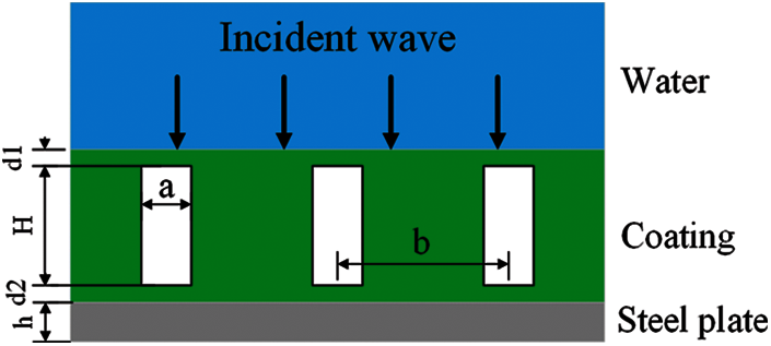
Figure 1: Viscoelastic coating structure of the cylindrical cavity
Table 1 shows the density, elastic modulus, loss factor and Poisson's ratio of the sound-absorbing layer used in this study as the input characteristic parameters.
By combining the values of the structural parameters of the coating given in Table 2 and the material parameters of the coating given in Table 1, based on the FEM, we performed a parametric scan on all combinations of the specified input characteristic parameters to solve the reflection coefficient of the viscoelastic coating containing a cylindrical cavity. The FEM is implemented on the platform with ANSYS v19.0. According to the literatures [14,36–38] regarding studies of the reflection coefficient of acoustic coatings, the consistency result of the reflection coefficient [6,14] is shown in Fig. 2.
2.2 Artificial Neural Network Model
ANNs establish the relationship between input variables and observation objects through neurons. The hidden layer usually contains multiple neurons, and the neurons between each layer are connected by weights [39]. The number of nodes in the hidden layer depends on the number of input nodes, the capacity of the training data, the complexity of the learning algorithm, and many other factors. More hidden layers and neurons may produce a model that is closer to the simulated training data. Notably, when the network is deeper, the ability to extract features is stronger; however, a neural network that contains too many hidden layers and neuron nodes is more likely to be overfitted, computationally expensive, and time-consuming to train [23]. Therefore, a compromise solution between accuracy and speed should be considered.
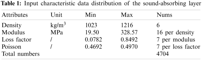
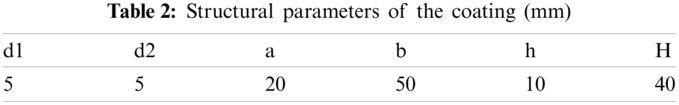
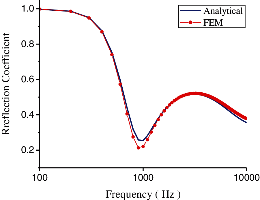
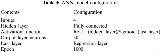
Figure 2: Comparison of the analytical and numerical solutions
In recent years, certain achievements have been made in the study of ANNs to predict the acoustic properties of different materials [26–30]. The ANN model structure with one hidden layer (ANN-1) is shown in Fig. 3. In several studies [27,29], ANN-1 was investigated to predict the acoustic properties of different material overlays. The ANN is based on a feedforward neural network, and the input layer of the ANN studied in this paper has four characteristics, namely, the density, elastic modulus, loss factor and Poisson's ratio. Since the reflection coefficient frequency varies from 200 to 6000 Hz and the interval is 200 Hz, there are 30 frequency points in total; therefore, we set the output layer as a fully connected layer of 30 neurons, and each neuron in the output layer corresponds to a frequency point one-by-one. After the output layer is activated, it is connected to the regression layer and returns the reflection coefficient of the viscoelastic acoustic coating containing a cylindrical cavity. Through the training and testing of the ANN, the regression prediction of the reflection coefficient is realized.
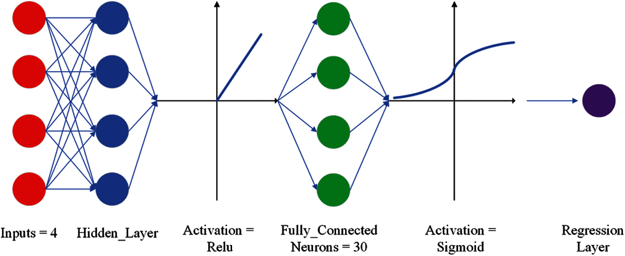
Figure 3: ANN-1 model structure for only one hidden layer
In the forward propagation of the ANN, the input samples are linearly fitted to the feature equation of the hidden layer to extract the input features, and then, the features are mapped to the (0, 1) value through the activation function [40]. The activation function introduces a nonlinear quantity to the neural network model so that the neural network can flexibly process complex data. Compared with activation functions such as sigmoid and tanh, the derivative of the rectified linear unit (ReLU) is 1, which effectively avoids gradient dispersion and gradient explosion [41]; therefore, it is often used in ANNs to stably minimize the loss function. The basic iterative process of forward propagation is as follows:
where X = (X1, X2, X3, X4) is a row vector that represents the characteristics of the input sample, which signifies the density, elastic modulus, loss factor, and Poisson's ratio. w is the weight matrix that connects the normalization value of the first layer to the hidden layer, and b is the bias vector obtained from the sample training. R is the vector obtained through σ mapping, and it represents the final predicted reflection coefficient result.
According to the input characteristic parameters given in Table 1, the reflection coefficient obtained by the FEM is used as the label value, and a total of 4704 tuples constitute the dataset. Since the inputs use different measurement units and their value ranges are not the same, the normalization preprocessing of the inputs is very important to the success of the model [42,43]. We used the minmax normalization method of Eq. (2) [44].
where X is the input feature parameter matrix, Xmin is the minimum value vector of each set of input feature parameters, and Xmax is the maximum value vector. The range of the calculated input element parameter Xscale for each set of calculations is dimensionless from −1 to 1; in this way, although the input feature parameters belong to different distributions or use different units of measurement, this normalization preprocessing method makes different input feature parameters comparable.
To evaluate the performance of the model, it is necessary to verify and test the model, and the process includes the ability to evaluate the model based on unused data. We divided the entire dataset into three subsets, specifically, a training dataset, a validation dataset and a test dataset. The training dataset is used to train the model, the validation dataset is used to observe the potential overfitting of the network during the training process, and the test dataset is used to evaluate the performance of the trained model. If the neural network model is overfitted during training, then it loses accuracy when it is simulated on the test dataset. We used 80% of the entire dataset as the training dataset, with a total of 3764 tuples, 10% as the validation dataset, with a total of 470 tuples, and the remaining 10% as the test dataset, with a total of 470 tuples. The test dataset specifies 48 tuples for the analysis of the reflection coefficient characteristics so that the ANN prediction results can be compared with the finite element results analysed in the first section. Except for the 48 tuples specified in the test dataset, the dataset division of the remaining tuples is random. It should be pointed out that since the input features are 4-dimensional data, we adopted the T-SNE [45] method to visualize them by using dimensionality reduction. Fig. 4 shows the distribution of the input features after dimensionality reduction.
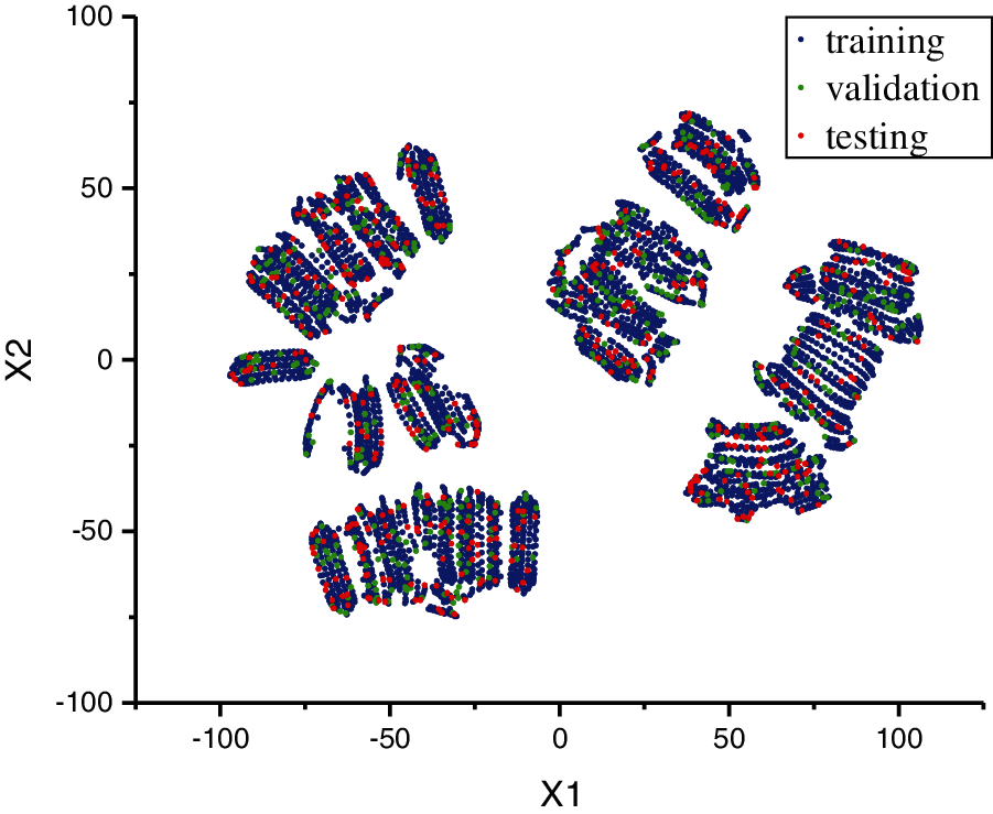
Figure 4: Distribution of the inputs. X1 and X2 are the two dimensions after dimension reduction
Table 3 shows the structure of the fully connected ANN model. Notably, since the range of the reflection coefficient output is a continuous value of [0, 1], the activation function used in the last layer is the sigmoid function.
For regression problems, we used the mean square error (MSE) method as the loss function [46].
where Rk is the k-th neural network in the L-th layer predicted value, which is calculated from the activation function of the last layer, and Ok is the k-th frequency ground truth value of the reflection coefficient that corresponds to the features of the input sample.
In back propagation, a gradient descent algorithm [47,48] is used to update the weight and bias to minimize the loss function. In training, we used a false bias and only need to update the gradient of the weight to minimize the MSE loss function during back propagation. According to the principle of back propagation, the gradient of the loss function of the last layer is Eq. (4)
where
It is known from (4) that the gradient of the j-th neuron in the previous (L − 1)-th layer connected to the k-th neuron in the L-th layer is only related to the activation function and the j-th neuron of the previous hidden layer.
For an ANN with multiple hidden layers, the gradient solution of the (L − 1)-th layer is calculated according to Eq. (5). Notably, the activation function of the hidden layer is ReLU, and its derivative is equal to 1.
From Eq. (5), the gradient of the h-th neuron in the (L−2)-th layer connected to the j-th neuron in the (L−1)-th layer is related to the weight and activation function of the k-th neuron in the L-th layer, and it is related to the output of the h-th neuron in the (L − 2)-th layer. According to the results of Eqs. (4) and (5), a recursive method is adopted to minimize the loss function by updating the ownership value of the neurons connected to each layer.
At present, ANNs have not yet seen effective and instructive methods to select the number of hidden layers, the number of neurons, the learning rate, the BatchSize and other hyperparameters. We used the grid search method to select the hyperparameters, as shown in Section 3.2.
2.5 Model Performance Evaluation
The performance evaluation of the neural network model is based on the classic performance indicators of the root mean square error (RMSE), mean absolute percentage error (MAPE) and Pearson correlation coefficient (PCC).
The RMSE [49,50] is calculated as Eq. (6).
where Oi is the i-th label value that corresponds to the input feature, Ri is the i-th predicted value, and N is 30 here, which represents the number of observed samples. The RMSE is a measure of the error between expected value data and model prediction data, which severely penalizes outliers. Since the RMSE is the square root of the MSE, it is the standard deviation of the residual between the value of the observed data and the estimated data, which means that the performance will decrease as the value increases. The RMSE adopts the unit of observation data; when the value is smaller, the model performance is better.
The MAPE [51,52] is calculated as Eq. (7).
where Oi is the i-th label value that corresponds to the input feature, Ri is the i-th predicted value, and N is 30 here, which represents the number of observed samples. The MAPE range is [0, 1), where 0 indicates a perfect model and 1 indicates an inferior model. When the value is smaller, the error is smaller. This error represents the average value of the absolute difference ratio between the actual observation value, and it is a linear score that balances all individual differences.
To directly measure the correlation between the predicted value of the model and the label value, we used the PCC [53,54] as Eq. (8).
where
3.1 Reflection Coefficient Characteristics of the FEM
First, we sampled and analysed the results of the FEM. The loss factor (0.325) and Poisson's ratio (0.476) remained unchanged. By changing the value of the elastic modulus, we sampled 4 sets of data with a density of 1068 kg/m3, as shown in Fig. 5a. When the elastic modulus is smaller, the reflection coefficient has more peaks and troughs in the frequency range. As the elastic modulus increases, the peaks and troughs move to high frequencies, the peaks gradually decrease, and the reflection coefficient finally forms a smooth curve. Subsequently, the same method was used to sample and analyse 12 sets of data with densities of 1106, 1142, and 1181 kg/m3, and the reflection coefficient in the frequency range changes with the elastic modulus, as shown in Figs. 5b–5d, respectively. When the density is different, the peak and trough frequencies of the reflection coefficient remain basically unchanged, their value changes very little, and the overall trend of the reflection coefficient curve does not change significantly. Accordingly, the elastic modulus is an important factor that influences the number and location of reflection coefficient peaks and troughs, while the density has little effect on the reflection coefficient.
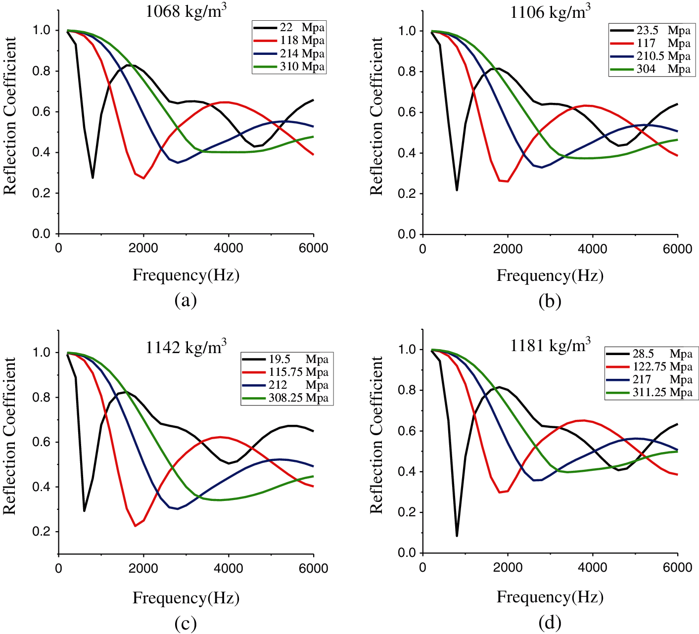
Figure 5: Sound reflection coefficient values of (a) 22, 118, 214, and 310 MPa modulus samples with a 1068 kg/m3 density, 0.325 loss factor, and 0.476 Poisson's ratio; (b) 23.5, 117, 210.5, and 310 MPa modulus samples with a 1106 kg/m3 density, 0.349 loss factor, and 0.4732 Poisson's ratio; (c) 19.5, 115.75, 212, and 308.25 MPa modulus samples with a 1142 kg/m3 density, 0.3844 loss factor, and 0.4706 Poisson's ratio; and (d) 28.5, 122.75, 217, and 311.25 MPa modulus samples with a 1181 kg/m3 density, 0.3228 loss factor, and 0.4692 Poisson's ratio
Then, the density (1068 kg/m3) and Poisson's ratio (0.476) remain unchanged, and by changing the value of the loss factor, we sampled 16 sets of data with elastic moduli of 22, 118, 214, and 310 MPa. Fig. 6 shows that the law of the reflection coefficient changes with the loss factor. When the loss factor is smaller, there are more peaks and troughs in the frequency range. As the loss factor increases, the peak value of the reflection coefficient decreases, the first valley decreases, and the frequency does not change. Due to the loss of sound energy by the loss factor, the peaks and troughs of the reflection coefficient curve are flattened, and the fluctuations in the curve become gentle. Accordingly, the loss factor is an important factor that influences the number of reflection coefficient peaks and troughs and the degree of curve fluctuations, but it does not affect the peak and trough frequencies.
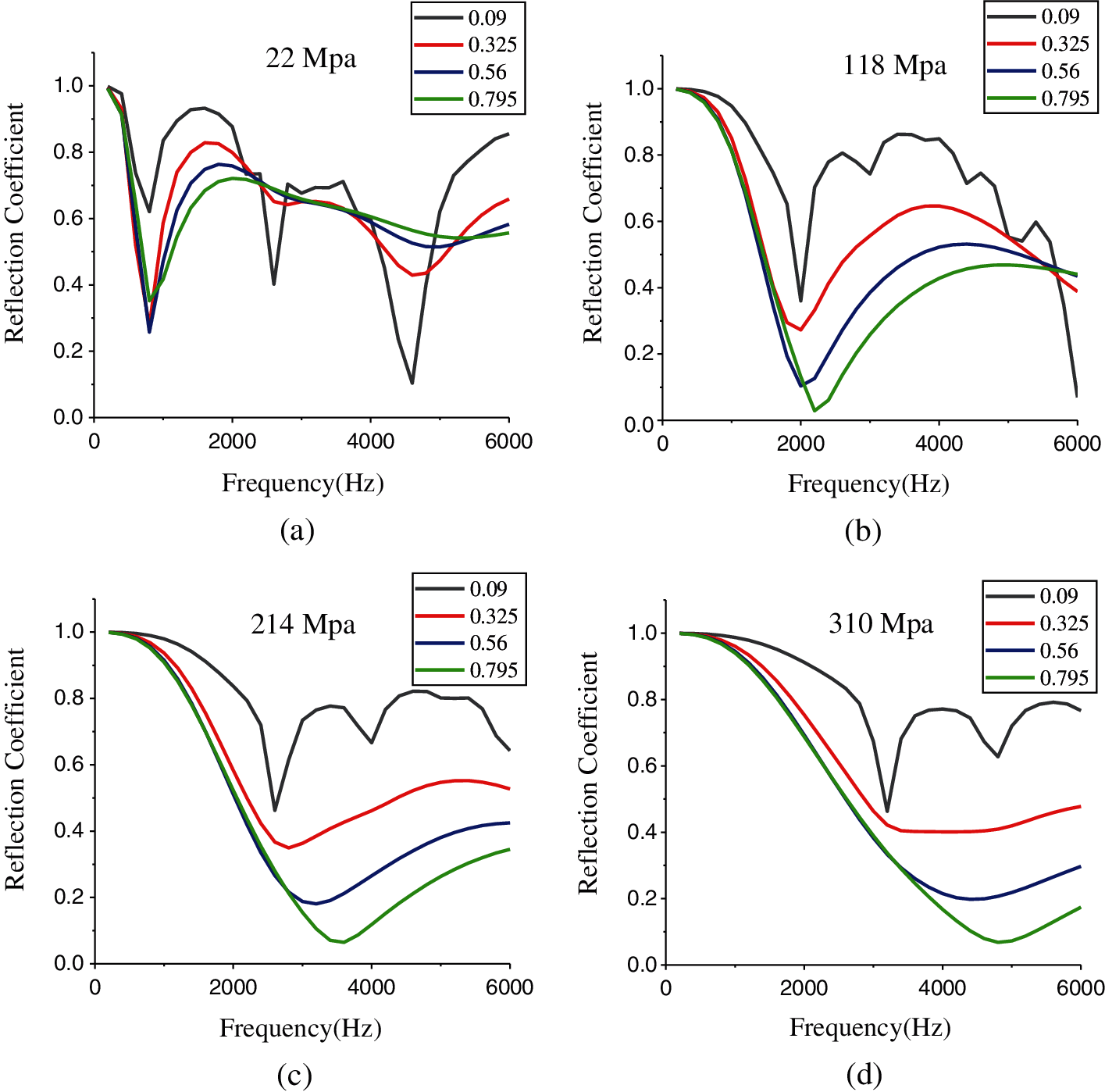
Figure 6: Sound reflection coefficient values for samples with a 1068 kg/m3 density, a 0.476 Poisson's ratio and 0.09, 0.325, 0.56, and 0.795 loss factors and (a) 22 MPa, (b) 118 MPa, (c) 214 MPa, and (d) 310 MPa moduli
Finally, by maintaining the density (1068 kg/m3) and the smaller loss factor (0.09) and changing the value of Poisson's ratio, we sampled 16 sets of data with elastic moduli of 22, 118, 214, and 310 MPa. Fig. 7 shows that the law of the reflection coefficient changes with Poisson's ratio. An analysis of the low frequency range below 2500 Hz in Fig. 7a shows that when Poisson's ratio changes, the peak-to-trough frequency of the reflection coefficient does not change, but the magnitude changes, as shown in Figs. 7b–7d. For frequency bands higher than 2500 Hz, although the peak and trough positions of the reflection coefficient change, the number does not decrease. Therefore, Poisson's ratio is an important factor that affects the peak and trough of the reflection coefficient. When the elastic modulus is smaller, Poisson's ratio has a greater impact on the peak and trough values of the reflection coefficient at low frequencies and a greater impact on the peaks, troughs and frequencies of the mid-to-high frequencies.
The above analysis shows that when the density, elastic modulus, loss factor and Poisson's ratio are used as the input characteristics of the viscoelastic acoustic coating, the acoustic performance of the coating is affected. Among them, the elastic modulus and loss factor are the key parameters for the acoustic performance of the coating and have a greater impact on the number and position of the reflection coefficient peaks and troughs in the frequency range and the fluctuation degree of the reflection coefficient curve. When their values are smaller, the characteristics of the reflection coefficient curve are more complicated.
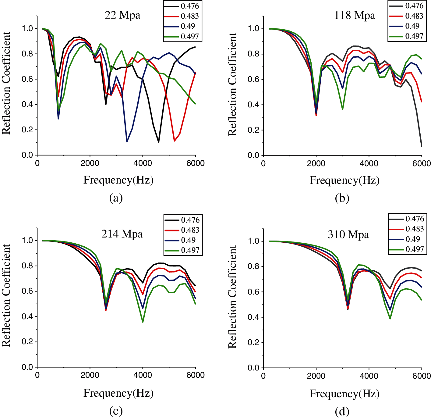
Figure 7: Sound reflection coefficient values of samples with a 1068 kg/m3 density, 0.09 loss factor, and 0.476, 0.483, 0.49, and 0.497 Poisson's ratios and for moduli of (a) 22 MPa, (b) 118 MPa, (c) 214 MPa, and (d) 310 MPa
3.2 Hyperparameters by the Grid Search Method
First, the learning rate and BatchSize are initialized to be 1e − 4 and 512, respectively, and the Adam learning algorithm is used to train the model. Fig. 8a shows the trends of the MSE training loss and verification loss with epochs for three neural network models with different depths of network layers and numbers of neurons. The MSE loss is drawn after completing each epoch training and verified once every 100 epochs; therefore, the training loss curve is relatively smooth. The selected hyperparameters are not overfitted in the model training. As the number of epochs increases, the MSE loss generally decreases; after 800 epochs are trained, the loss remains almost unchanged. When the network layer is deeper and the number of neurons is greater, the model converges faster, and the loss is smaller. ANN-9 has the fastest convergence speed and the smallest loss.
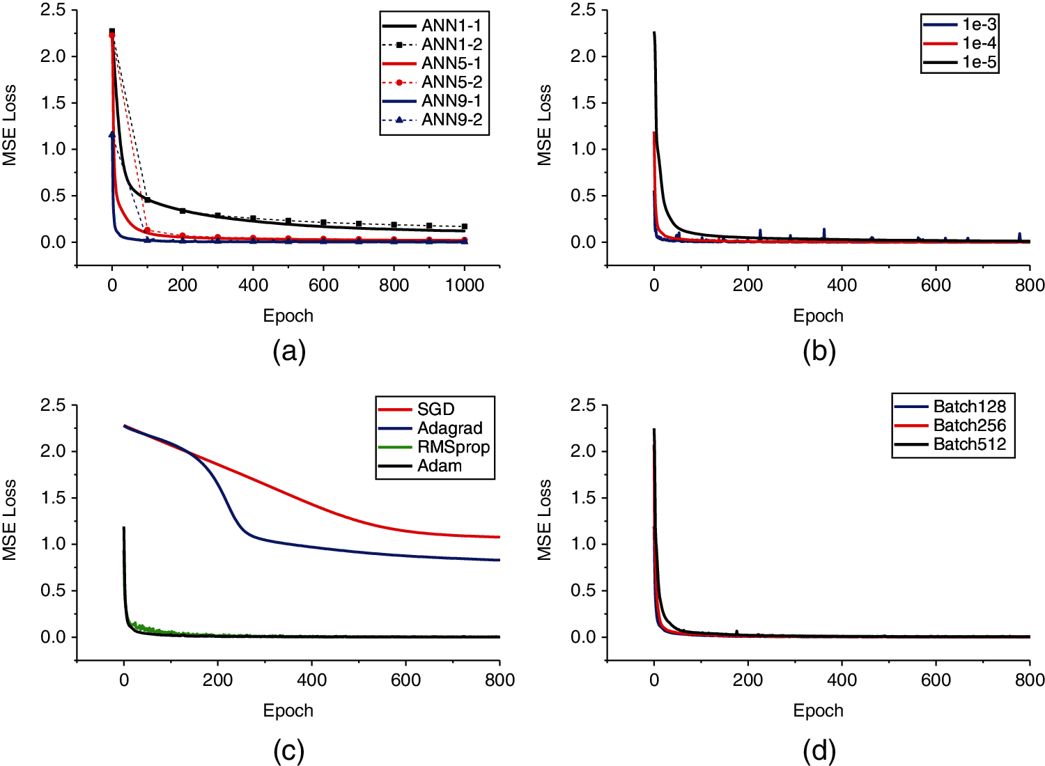
Figure 8: (a) Updating process of the MSE loss function. ANN1-1 and ANN1-2 represent the training loss and verification loss for one hidden layer (64 neurons), respectively. ANN5-1 and ANN5-2 represent the training loss and verification loss for five hidden layers (the number of neurons in each layer is 256, 128, 64, 128, and 256, respectively). ANN9-1 and ANN9-2 represent the training and verification losses for nine hidden layers (1024, 512, 256, 128, 64, 128, 256, 512, and 1024 neurons, respectively). (b) Trend of the MSE training loss with epochs for three different learning rate values. (c) The trend of the MSE training loss with epochs for four different optimizers. (d) The trend of the MSE training loss with epochs for three different BatchSizes
On the basis of ANN-9, we continued to train the model by changing the value of the learning rate. Fig. 8b shows the trend of the MSE training loss with epochs for three different learning rate values. When the learning rate is too large, the MSE loss curve oscillates more severely, which indicates that a larger learning rate may cause the model to fall into a local minimum, and when the learning rate is too small, the convergence speed will be slower. When the learning rate is 1e − 4, both convergence efficiency and stability are considered.
We change the different learning algorithms to continue training ANN-9. Fig. 8c shows the trend of the MSE training loss with epochs for four optimizers, including Adam with moment. The SGD optimizer and Adagrad optimizer have a slower convergence speed and a larger MSE loss. Although RMSprop converges faster during training, it continues to oscillate during the process. Adam with the moment algorithm has the smallest loss, the highest convergence efficiency, and the best stability. The Adam optimizer is the optimal algorithm suiTab. for research.
Finally, we continued to train the ANN-9 model by changing the value of BatchSize to 128, 256 and 512. Fig. 8d shows the trend of the MSE loss of different BatchSizes with epochs. When BatchSize is 128, the convergence speed and MSE loss are equivalent to BatchSize 256. To improve batch processing efficiency, we finally chose BatchSize to be 256.
The optimal hyperparameters are selected by the above grid search method, and the optimal hyperparameter configuration of our improved ANN model (ANN-ours) is shown in Table 4.
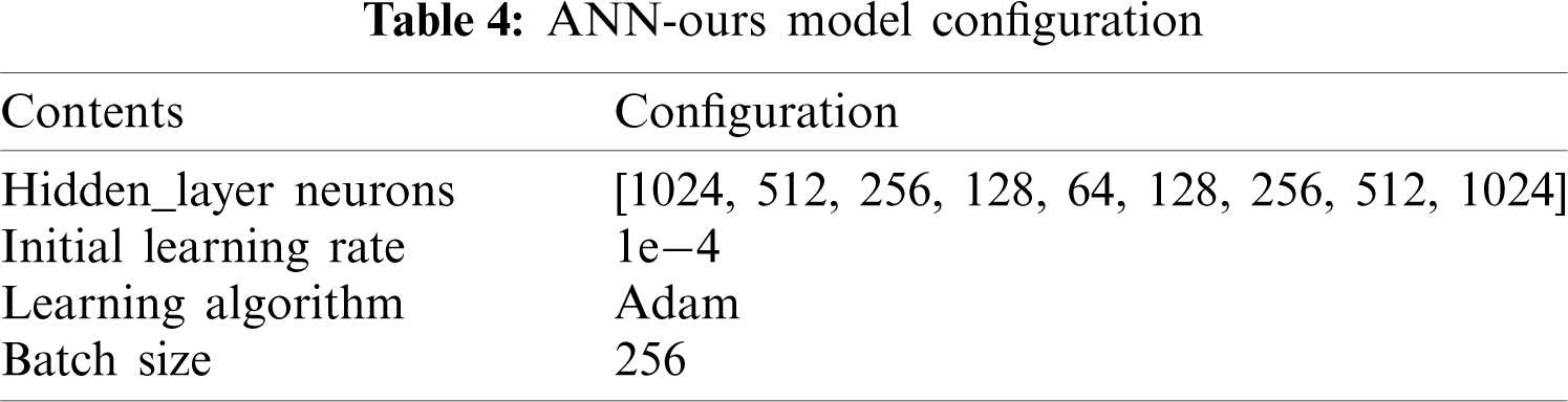
Fig. 9 shows the 10-fold cross-validation error that varies with epochs when the ANN-ours model is under the configuration of Table 4. With increasing epochs, the average RMSE prediction error of ANN-ours decreases. The average RMSE of 800 training epochs is 0.319, which ranges from 0.234 to 0.413, and the average RMSE of 1000 training epochs is 0.298, which ranges from 0.217 to 0.374. The 10-fold cross-validation RMSE shows that the error changes very little after 800 epochs. The range of the cross-validation error implies that the result of a single folding will lead to an underestimation or overestimation of prediction errors, and to save time, a reasonable epoch value should be chosen for training.
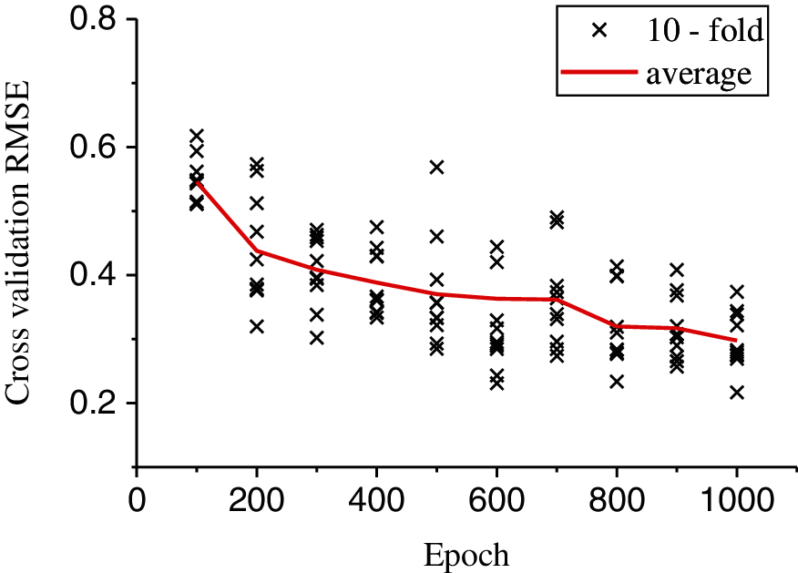
Figure 9: ANN-ours prediction of the reflection coefficient for the epoch and cross-validation RMSE
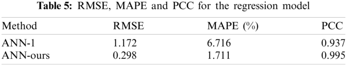
Table 5 compares the results of ANN-1 and ANN-ours. The average RMSE and MPAE values of the reflection coefficient simulated by ANN-ours are 0.298% and 1.711%, respectively, which are nearly 3.9 times higher than those of ANN-1, which shows that ANN-ours has a higher prediction accuracy. The PCC is 0.995, which means that the predicted value is closer to the label value.
3.4 Comparison of the ANN and FEM
We first compare the prediction values by ANN-ours with the 16 sets of FEM results in Fig. 5, and the comparative result is shown in Fig. 10. When the elastic modulus is small, the reflection coefficient has more peaks and troughs, and the predicted value of ANN-ours has a certain error at the troughs. As the elastic modulus increases, the error between the predicted value and the label value decreases. Even though the density increases or decreases, the prediction effect is basically unchanged.
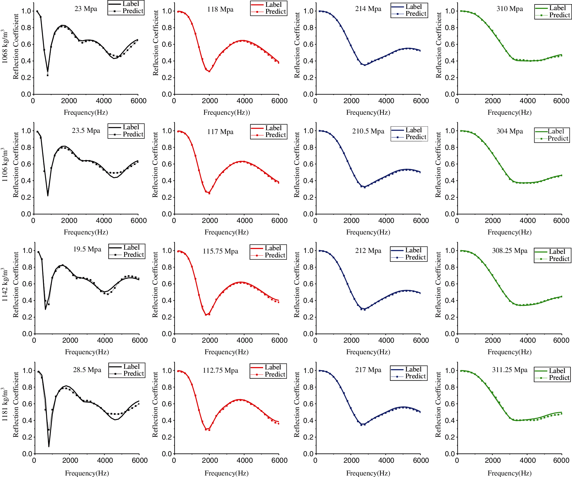
Figure 10: By changing the elastic modulus value, the trend of the acoustic reflection coefficient with the frequency predicted by the FEM and ANN-ours. The solid curve represents the finite element simulation value, and the symbolic curve represents the ANN-our predicted value
Then, we compare the 16 sets of reflection coefficients solved by FEM in Fig. 6 with the prediction values of ANN-ours. As shown in Fig. 11, when the loss factor is smaller, the reflection coefficient has more peaks and troughs, the fluctuation of the curve is greater, and the error further increases at the peaks and troughs. As the loss factor increases, the error decreases, and the reflection coefficient curve predicted by ANN-ours fits the label value curve better.
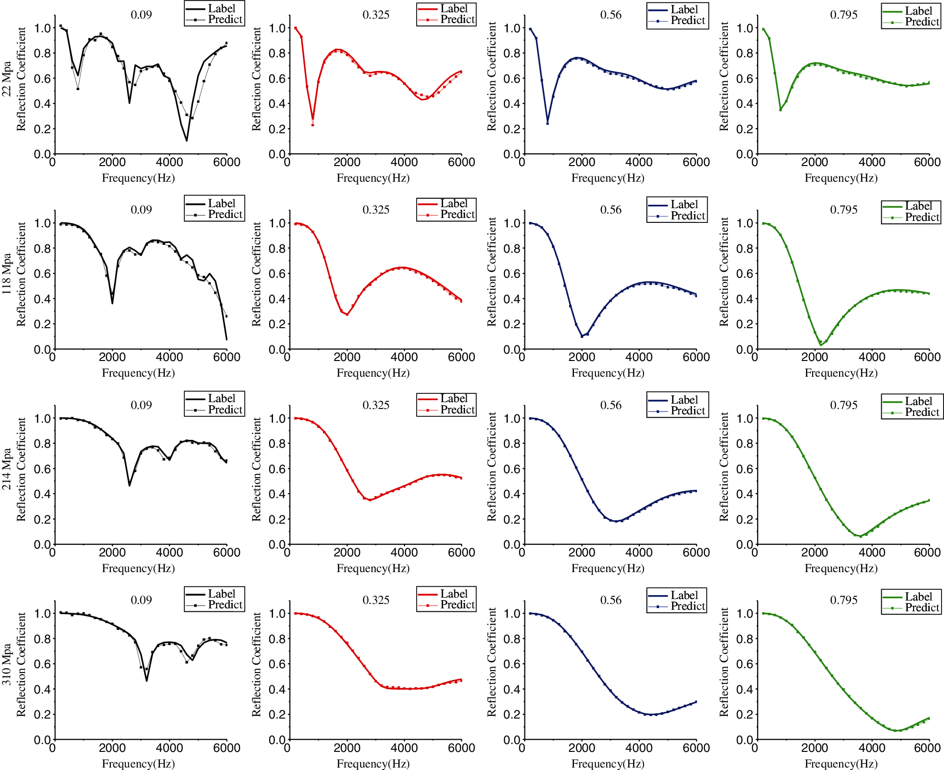
Figure 11: By changing the loss factor value, the trend of the acoustic reflection coefficient with the frequency predicted by the FEM and ANN-ours. The solid curve represents the finite element simulation value, and the symbolic curve represents the ANN-ours predicted value
Finally, we compared the 16 groups of reflection coefficients in Fig. 7 with ANN-ours. As shown in Fig. 12, although the predicted reflection coefficient curve and the label value curve have the same overall change trend, the errors at the peaks and troughs are relatively large, especially when the elastic modulus and loss factor are very small, and the error is the largest. It should be pointed out that the increase or decrease of Poisson's ratio does not significantly change the prediction effect of ANN-ours.
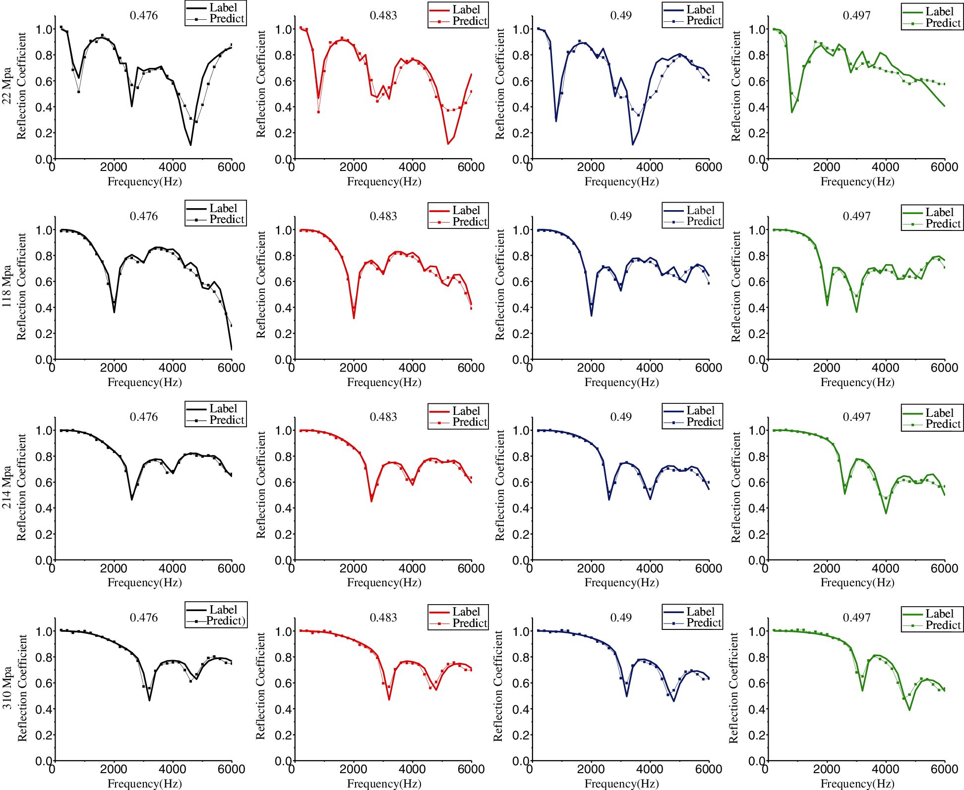
Figure 12: By changing the Poisson ratio value, the trend of the acoustic reflection coefficient with the frequency predicted by the FEM and ANN-ours. The solid curve represents the finite element simulation value, and the symbolic curve represents the ANN predicted value
Through the analysis of the above results, the following conclusions can be drawn. When the elastic modulus and loss factor are smaller, the number of peaks and troughs of the reflection coefficient is greater, the fluctuation of the curve is larger, and the prediction effect based on ANN-ours is worse. The reason is that the features of the reflection coefficient are the most complicated in this case, and ANN-ours has not yet learned advanced features.
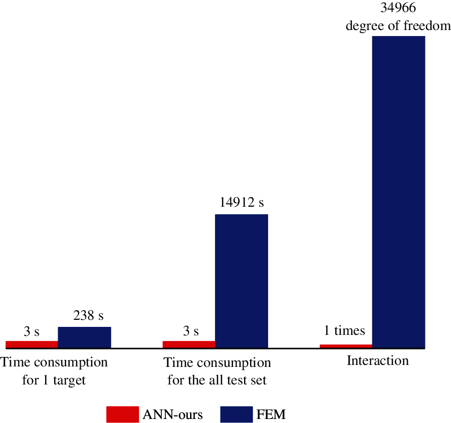
Figure 13: Time consumption and calculation iteration comparisons of the ANN-ours and FEM
In this paper, a data-based ANN model is investigated to accurately and efficiently predict the reflection coefficient of a viscoelastic acoustic coating containing a cylindrical cavity. This method, which has great innovation, overcomes the disadvantages of the high experimental cost of measuring the reflection coefficient and the time-consuming calculation of the finite element analysis in the traditional methods. Comparisons of the ANN-ours and FEM are shown in Fig. 13. The times required for the ANN-ours and FEM to obtain one reflection coefficient are 3 and 238 s, respectively. The ANN-ours is nearly 79 times faster than the FEM. Moreover, because ANN-ours is an end-to-end deep learning model, the number of iterations is only one, and the FEM needs to iteratively solve 34966 degrees of freedom. Due to its batch processing and end-to-end learning capabilities, the ANN model could further improve the prediction efficiency when predicting multiple acoustic targets.
First, a reflection coefficient feature dataset based on the FEM was generated, and the minmax normalization preprocessing method was performed on the data. The FEM of generating the dataset avoids repeated experiments. Then, the 10-fold cross-validation error was calculated, and the prediction results of the acoustic reflection coefficient of ANN-ours and the ANN-1 regression model were compared. The average RMSE and MAPE predicted by ANN-ours were lower, and the PCC was higher.
The research results in this paper show that ANN-ours improves the predictive power when evaluating the acoustic performance of a viscoelastic acoustic coating containing a cylindrical cavity and allows it to be used to simulate the reflection coefficient of configurations where acoustic measurements are not available, which may be particularly important for certain applications. The ANN-ours model requires less professional knowledge in the field of acoustics. It provides an effective tool for engineering and technical personnel, and these users only need to focus on developing the material parameters of the expected acoustic performance design goals rather than spending much time solving the numerical model. Specifically, the reflection coefficient of the viscoelastic acoustic coating containing a cylindrical cavity in the frequency range from 200 to 6000 Hz is determined by the well-trained ANN according to the density, elastic modulus, loss factor and Poisson's ratio. Table 5 compares the prediction results of ANN-ours and ANN-1. As the ANN-ours network has deeper layers and more neurons and as the hyperparameters are fine-tuned by the grid search method, it has better estimation accuracy than the ANN-1 model.
Notably, the ANN model in this study only uses the overlay parameter dataset under hard sound field boundary conditions for training. Although the result provides a positive starting point for future research, ANN models that require more types of input features are needed for future work. Therefore, a database that contains more extensive data is needed to expand the range of acoustic coatings to which the model can be applied. Further research will focus on collecting more data from samples of acoustic coatings with different structures, a wider range of thicknesses, cavity dimensions and backing sound-absorbing layers. By expanding the database, it is possible to more widely evaluate the acoustic performance of the coating under different materials and cavity rules, thereby reducing the time and effort required to measure the nonacoustic parameters of the coating. In addition, it is also possible to design an ANN model that covers complex cavity features because it is usually difficult to use theoretical methods to accurately obtain the acoustic performance of the acoustic coating on a complex cavity scale, it is difficult to produce complex cavity-scale samples of the coating, and experimental methods are too costly.
In the future, based on the results obtained in our previous work, a high-efficiency inversion method for the material and structure parameters and a rapid prediction of the acoustic performance of viscoelastic coatings that contain cavities are the goals of our next research. We will research this topic as a pavement for the active and adaptive control of sound and vibration.
Acknowledgement: We would like to thank Cunhong Yin and other members of the material team for their helpful discussions. We thank the developers of TensorFlow 2.0, which we used for all of our experiments.
Availability of Data and Materials: The dataset and code for this article can be found online at https://github.com/sunyiping1987/Paper.git.
Funding Statement: This work was supported by the National Natural Science Foundation of China (Nos. 51765008 and 11304050), the High-Level Innovative Talents Project of Guizhou Province (No. 20164033), the Science and Technology Project of Guizhou Province (No. 2020-1Z048), and the Open Project of the Key Laboratory of Modern Manufacturing Technology of the Ministry of Education (No. XDKFJJ [2016]10).
Conflicts of Interest: The authors declare that they have no known competing financial interests or personal relationships that could have appeared to influence the work reported in this paper.
1. Zieliński, T. G., Chevillotte, F., Deckers, E. (2018). Sound absorption of plates with micro-slits backed with air cavities: Analytical estimations, numerical calculations and experimental validations. Applied Acoustics, 146(3), 261–279. DOI 10.1016/j.apacoust.2018.11.026. [Google Scholar] [CrossRef]
2. Jin, G., Shi, K., Ye, T., Zhou, J., Yin, Y. (2020). Sound absorption behaviors of metamaterials with periodic multi-resonator and voids in water. Applied Acoustics, 166(9), 107351. DOI 10.1016/j.apacoust.2020.107351. [Google Scholar] [CrossRef]
3. Wang, S., Hu, B., Du, Y. (2020). Sound absorption of periodically cavities with gradient changes of radii and distances between cavities in a soft elastic medium. Applied Acoustics, 170(12), 107501. DOI 10.1016/j.apacoust.2020.107501. [Google Scholar] [CrossRef]
4. Wang, X., Ma, L., Wang, Y., Guo, H. (2021). Design of multilayer sound-absorbing composites with excellent sound absorption properties at medium and low frequency via constructing variable section cavities. Composite Structures, 266(12), 113798. DOI 10.1016/j.compstruct.2021.113798. [Google Scholar] [CrossRef]
5. Liu, X., Yu, C., Xin, F. (2021). Gradually perforated porous materials backed with Helmholtz resonant cavity for broadband low-frequency sound absorption. Composite Structures, 263(10), 113647. DOI 10.1016/j.compstruct.2021.113647. [Google Scholar] [CrossRef]
6. Tang, W., He, S., Fan, J. (2005). Two-dimensional model for acoustic absorption of viscoelastic coating containing cylindrical holes. Acta Acustica, 30(4), 289–295. [Google Scholar]
7. Wang, R. (2004). Methods to calculate an absorption coefficient of sound-absorber with cavity. Acta Acustica, 29(5), 393–397. [Google Scholar]
8. Tang, W. (1993). Calculation of acoustic scattering of a nonrigid surface using physical acoustic method. Chinese Journal of Acoustics, 12(1), 226–234. [Google Scholar]
9. Fan, J., Zhu, B., Tang, W. (2001). Modifled geometrical highlight model of echoes from nonrigid sonar target. Acta Acustica, 26(6), 545–550. DOI 10.1038/sj.cr.7290097. [Google Scholar] [CrossRef]
10. Easwaran, V., Munjal, M. L. (1993). Analysis of reflection characteristics of a normal incidence plane wave on resonant sound absorbers: A finite element approach. Journal of the Acoustical Society of America, 93(3), 1308–1318. DOI 10.1121/1.405416. [Google Scholar] [CrossRef]
11. Panigrahi, S. N., Jog, C. S., Munjal, M. L. (2007). Multi-focus design of underwater noise control linings based on finite element analysis. Applied Acoustics, 69(12), 1141–1153. DOI 10.1016/j.apacoust.2007.11.012. [Google Scholar] [CrossRef]
12. Ivansson, S. M. (2006). Sound absorption by viscoelastic coatings with periodically distributed cavities. Journal of the Acoustical Society of America, 119(6), 3558–3567. DOI 10.1121/1.2190165. [Google Scholar] [CrossRef]
13. Ivansson, S. M. (2008). Numerical design of Alberich anechoic coatings with superellipsoidal cavities of mixed sizes. Journal of the Acoustical Society of America, 124(4), 1974–1984. DOI 10.1121/1.2967840. [Google Scholar] [CrossRef]
14. Tao, M., Zhou, L. (2011). Simulation and analysis for acoustic performance of a sound absorption coating using ANSYS software. Journal of Vibration and Shock, 30(1), 87–90. DOI 10.1109/EPE.2015.7161153. [Google Scholar] [CrossRef]
15. Yu, Y., Xu, H., Xie, X., Li, S. (2017). Optimization design of underwater anechonic coating structural parameters using MPGA. Science Technology and Engineering, 17(2), 5–10. DOI CNKI: SUN: KXJS.0.2017-02-002. [Google Scholar]
16. Huang, L., Xiao, Y., Wen, J., Zhang, H., Wen, X. (2018). Optimization of decoupling performance of underwater acoustic coating with cavities via equivalent fluid model. Journal of Sound and Vibration, 426(28), 244–257. DOI 10.1016/j.jsv.2018.04.024. [Google Scholar] [CrossRef]
17. Zhao, D., Zhao, H., Yang, H., Wen, J. (2018). Optimization and mechanism of acoustic absorption of alberich coatings on a steel plate in water. Applied Acoustics, 140(11), 183–187. DOI 10.1016/j.apacoust.2018.05.027. [Google Scholar] [CrossRef]
18. Deng, G., Shao, J., Zheng, S., Wu, X. (2020). Optimal study on sectional geometry of rubber layers and cavities based on the vibro-acoustic coupling model with a sine-auxiliary function. Applied Acoustics, 170(12), 107522. DOI 10.1016/j.apacoust.2020.107522. [Google Scholar] [CrossRef]
19. Bai, C., Chen, T., Wang, X., Sun, X. (2021). Optimization layout of damping material using vibration energy-based finite element analysis method. Journal of Sound and Vibration, 504(28), 116117. DOI 10.1016/j.jsv.2021.116117. [Google Scholar] [CrossRef]
20. Yang, C., Lan, H., Gao, F., Gao, F. (2021). Review of deep learning for photoacoustic imaging. Photoacoustics, 21(1), 100215. DOI 10.1016/j.pacs.2020.100215. [Google Scholar] [CrossRef]
21. Yuan, S., Wu, X. (2021). Deep learning for insider threat detection: Review, challenges and opportunities. Computers & Security, 104(3), 102221. DOI 10.1016/j.cose.2021.102221. [Google Scholar] [CrossRef]
22. Janek, G., Melanie, S., Kris, D., Lena, M. (2021). Deep learning for biomedical photoacoustic imaging: A review. Photoacoustics, 22(2), 100241. DOI 10.1016/j.pacs.2021.100241. [Google Scholar] [CrossRef]
23. Lecun, Y., Bengio, Y., Hinton, G. (2015). Deep learning. Nature, 521(7553), 436–444. DOI 10.1038/nature14539. [Google Scholar] [CrossRef]
24. Stanley, C., Benjamin, R. M. (2021). Chapter 3-Overview of advanced neural network architectures. Artificial intelligence and deep learning in pathology. TNQ Technologies, India: Dolores Meloni. [Google Scholar]
25. Gad, A. F., Jarmouni, F. E. (2021). Chapter 2-Introduction to artificial neural networks (ANN). Introduction to deep learning and neural networks with Python™. SPi Global, India: Nikki Levy. [Google Scholar]
26. Lin, M., Tsai, K., Su, B. (2008). Estimating the sound absorption coefficients of perforated wooden panels by using artificial neural networks. Applied Acoustics, 70(1), 31–40. DOI 10.1016/j.apacoust.2008.02.001. [Google Scholar] [CrossRef]
27. Iannace, G., Ciaburro, G., Trematerra, A. (2020). Modelling sound absorption properties of broom fibers using artificial neural networks. Applied Acoustics, 163(6), 107239. DOI 10.1016/j.apacoust.2020.107239. [Google Scholar] [CrossRef]
28. Jeon, J. H., Yang, S. S., Kang, Y. J. (2020). Estimation of sound absorption coefficient of layered fibrous material using artificial neural networks. Applied Acoustics, 169(12), 107476. DOI 10.1016/j.apacoust.2020.107476. [Google Scholar] [CrossRef]
29. Ciaburro, G., Iannace, G., Passaro, J., Bifulco, A., Marano, A. D. et al. (2020). Artificial neural network-based models for predicting the sound absorption coefficient of electrospun poly (vinyl pyrrolidone)/silica composite. Applied Acoustics, 169(12), 107472. DOI 10.1016/j.apacoust.2020.107472. [Google Scholar] [CrossRef]
30. Paknejad, S. H., Vadood, M., Soltani, P., Ghane, M. (2020). Modeling the sound absorption behavior of carpets using artificial intelligence. Journal of the Textile Institute, 111(11), 1–9. DOI 10.1080/00405000.2020.1841954. [Google Scholar] [CrossRef]
31. He, S., Tang, W., Fan, J. (2005). Axisymmetric wave propagation and attenuation along an infinite viscoelastic cylindrical tube. Acta Acustica, 30(3), 249–254. [Google Scholar]
32. Wang, R., Ma, L. (2004). Effects of physical parameters of the absorption material on absorption capability of anechoic tiles. Journal of Harbin Engineering University, 25(3), 288–294. DOI 10.3969/j.issn.1006-7043.2004.03.006. [Google Scholar] [CrossRef]
33. Luo, Y., Luo, J., Zhang, Y., Li, J. (2021). Sound-absorption mechanism of structures with periodic cavities. Acoustics Australia, 49(1), 371–383. DOI 10.1007/s40857-021-00233-6. [Google Scholar] [CrossRef]
34. Yuan, S., Li, S., Zhu, J., Tang, Y. (2021). Additive manufacturing of polymeric composites from material processing to structural design. Composites Part B Engineering, 219(4), 108903. DOI 10.1016/j.compositesb.2021.108903. [Google Scholar] [CrossRef]
35. Krishna, R., Manjaiah, M., Mohan, C. B. (2021). Chapter 3-Developments in additive manufacturing. Additive manufacturing. MPS Limited, Chennai, India: Matthew Deans. [Google Scholar]
36. Ye, H., Tao, M., Li, J. (2019). Sound absorption performance analysis of anechoic coatings under oblique incidence condition based on COMSOL. Journal of Vibration and Shock, 38(12), 213–218. DOI CNKI: SUN: ZDCJ.0.2019-12-030. [Google Scholar]
37. Ke, L., Liu, C., Fang, Z. (2020). COMSOL-Based acoustic performance analysis of combined cavity anechoic layer. Chinese Journal of Ship Research, 15(5), 167–175. DOI 10.19693/j.issn.1673-3185.01673. [Google Scholar] [CrossRef]
38. Liu, X. W. (2019). Calculation and analysis of cavity in sound insulation layer based on sound absorbing material. Huazhong University of Science and Technology. DOI 10.27157/d.cnki.ghzku.2019.002249. [Google Scholar] [CrossRef]
39. Schilling, F. P., Stadelmann, T. (2020). Structured (De)composable representations trained with neural networks. Artificial neural networks in pattern recognition. Germany: Springer. [Google Scholar]
40. Gulcehre, C., Moczulski, M., Denil, M., Bengio, Y. (2016). Noisy activation functions. Proceedings of the 33rd International Conference on Machine Learning, vol. 48, pp. 3059–3068. [Google Scholar]
41. Nair, V., Hinton, G. E. (2010). Rectified linear units improve restricted boltzmann machines vinod nair. Proceedings of the 27th International Conference on Machine Learning, pp. 807–814. Haifa, Israel, Omnipress. [Google Scholar]
42. Kaplinski, O., Tamošaitienė, J. (2015). Analysis of normalization methods influencing results: A review to honour professor friedel peldschus on the occasion of his 75th birthday. Procedia Engineering, 122, 2–10. [Google Scholar]
43. Simon, O. H. (2008). Chapter 4-Regularization theory. Neural networks and learning machines. New Jersey: Pearson. [Google Scholar]
44. Hang, C. X., Ivan, S., Zoran, O. (2016). A robust data scaling algorithm to improve classification accuracies in biomedical data. BMC Bioinformatics, 17(359), 1–10. DOI 10.1186/s12859-016-1236-x. [Google Scholar] [CrossRef]
45. Laurens, V. D. M., Hinton, G. (2008). Visualizing data using t-SNE. Journal of Machine Learning Research, 9(86), 2579–2605. [Google Scholar]
46. Martin-Donas, J. M., Gomez, A. M., Gonzalez, J. A. et al. (2018). A deep learning loss function based on the perceptual evaluation of the speech quality. IEEE Signal Processing Letters, 25(11), 1680–1684. DOI 10.1109/LSP.2018.2871419. [Google Scholar] [CrossRef]
47. Sharma, A. (2018). Guided stochastic gradient descent algorithm for inconsistent datasets. Applied Soft Computing, 73(4), 1068–1080. DOI 10.1016/j.asoc.2018.09.038. [Google Scholar] [CrossRef]
48. Xiao, W. (2017). Introduction to gradient descent algorithm (along with variants) in machine. https://www.cnblogs.com/wangxiaocvpr/p/6532691.html. [Google Scholar]
49. Calasan, M., Abdel Aleem, S. H. E., Zobaa, A. F. (2020). On the root mean square error (RMSE) calculation for parameter estimation of photovoltaic models: A novel exact analytical solution based on Lambert W function. Energy Conversion and Management, 210(8), 112716. DOI 10.1016/j.enconman.2020.112716. [Google Scholar] [CrossRef]
50. Hebeler, F. (2021). MATLAB central file exchange. https://www.mathworks.com/matlabcentral/fileexchange/21383-rmse. [Google Scholar]
51. Arnaud de, M., Boris, G., Bénédicte, L. G., Fabrice, R. (2015). Mean absolute percentage error for regression models. Neurocomputing, 192(3), 38–48. DOI 10.1016/j.neucom.2015.12.114. [Google Scholar] [CrossRef]
52. Kim, S., Kim, H. (2016). A new metric of absolute percentage error for intermittent demand forecasts. International Journal of Forecasting, 32(3), 669–679. DOI 10.1016/j.ijforecast.2015.12.003. [Google Scholar] [CrossRef]
53. Fu, T., Tang, X. B., Cai, Z. K., Zuo, Y., Tang, Y. M. et al. (2019). Correlation research of phase angle variation and coating performance by means of Pearson's correlation coefficient. Progress in Organic Coatings, 139(2), 105459. DOI 10.1016/j.porgcoat.2019.105459. [Google Scholar] [CrossRef]
54. Edelmann, D., Móri, T. F., Székely, G. J. (2021). On relationships between the Pearson and the distance correlation coefficients. Statistics & Probability Letters, 169(3), 108960. DOI 10.1016/j.spl.2020.108960. [Google Scholar] [CrossRef]
 | This work is licensed under a Creative Commons Attribution 4.0 International License, which permits unrestricted use, distribution, and reproduction in any medium, provided the original work is properly cited. |