Computer Modeling in Engineering & Sciences

DOI: 10.32604/cmes.2022.018450

ARTICLE

Estimating Daily Dew Point Temperature Based on Local and Cross-Station Meteorological Data Using CatBoost Algorithm

Fuqi Yao1, Jinwei Sun1 and Jianhua Dong2,*

1School of Hydraulic Engineering, Ludong University, Yantai, 264010, China
2State Key Laboratory of Water Resources and Hydropower Engineering Science, Wuhan University, Wuhan, 430072, China
*Corresponding Author: Jianhua Dong. Email: djh0530dyz@126.com
Received: 25 July 2021; Accepted: 25 August 2021

1  Introduction

Dew point temperature (Tdew) is the temperature at which water vapor in the air condenses into water droplets. Accurate estimation of Tdew data plays a significant role in the fields of energy utilization [1], thermal energy [2,3] and engineering [4]. Tdew is also an essential parameter for studying long-term climate change [5,6]. Tdew is usually used in conjunction with relative humidity to calculate the water content in the air [7]. It can be also combined with the wet bulb temperature to calculate the ambient temperature to prevent crop frost in advance and reduce the risk of crop yield reduction [8]. In many fields, Tdew is needed to estimate reference crop evapotranspiration (ET0) [9]. Tdew also affects human life safety and living environment comfort during the heatwave [10]. Compared with other meteorological variables, Tdew is still relatively inadequate. Because of its importance and non-linear changes, accurate estimation of Tdew has vital scientific significance in the above fields.

Compared with traditional meteorological parameters (such as temperature, precipitation and sunshine duration), Tdew is relatively more challenging to obtain. This is because some weather stations cannot measure Tdew normally. Scholars have mainly used traditional regression techniques to estimate Tdew [11], but the estimated data had significant errors and certain uncertainties. To better solve the problem of incomplete Tdew data, scholars have proposed various methods to estimate Tdew. In recent years, machine learning algorithms have been used to estimate various parameters and recognise images (including snow cover area, leaf area index (LAI), Tdew and image classification etc.) with excellent performance [12–17]. Kuter [14] estimated the snow cover over parts of the European Alps using remote sensing data combined with multiple adaptive regression spline (MARS), support vector regression (SVR), random forests (RF) and artificial neural network (ANN) algorithms. He concluded that MARS and RF algorithms would outperform ANN and SVR algorithms in terms of estimation performance and computational cost. Houborg et al. [15] obtained satisfactory results for estimating LAI by hybridizing the Cubist and RF algorithm. Because of their excellent performance in handling the non-linear relationships between inputs and output, e.g., ANN, MARS, RF, adaptive neural fuzzy inference system (ANFIS), support vector machine (SVM), extreme learning machine (ELM) and gene expression programming (GEP).

Among the above machine learning algorithms, ANN is the earliest and widely used algorithm. Shank et al. [18] applied the ANN algorithm with meteorological data from 20 weather stations in Georgia of USA to estimate Tdew within the next 1–12 h and established a general algorithm. They demonstrated that ANN had satisfactory accuracy in estimating Tdew. Zounemat-Kermani et al. [19] studied the potential of multilinear regression (MLR) and Levenberg-Marquardt neural network (LM-NN) in Ontario of Canada to estimate hourly Tdew. It was found that LM-NN had better performance than the MLR algorithm. Shiri et al. [20] coupled the ANN and GEP algorithms to estimate Tdew in Seoul and Incheon of South Korea and found that the ANN algorithm had excellent estimation capability. Still, the performance of the GEP algorithm was better than the ANN algorithm. Nadig et al. [21] implemented single and hybrid ANN algorithms to estimate air temperature and Tdew. They concluded that the hybrid algorithm could effectively improve the estimation stability, and the average error was decreased by 34.1%. The ANFIS algorithm was also often used to estimate Tdew. Mohammadi et al. [22] applied the ANFIS algorithm to estimate Tdew at Kerman and Tabas stations in Iran. They found that water vapor pressure (Vp) and RH were the most relevant and irrelevant meteorological parameters, respectively. Kisi et al. [23] evaluated several combined algorithms such as the ANFIS algorithm with sub-clustering identification (ANFIS-SC) and ANFIS algorithm with grid partitioning identification (ANFIS-GP) to estimate daily Tdew at three stations in South Korea. They indicated that the accuracy of these two algorithms was very close, and they were better than the other studied algorithms.

Baghban et al. [24] evaluated the genetic algorithm (GA)-optimized least squares support vector machine (LSSVM) and ANFIS algorithm to estimate Tdew, and found that these two algorithms had high accuracy and stability. The MARS algorithm's advantage is that it can handle big data with high dimensions with short computational time and high prediction accuracy. Therefore, it has been used in many fields. Dong et al. [25] estimated daily diffuse solar radiation (Rd) at five stations in China using MARS and SVM. The results confirmed that the MARS algorithm had an excellent performance in estimating Rd. Wu et al. [26] applied MARS, ANFIS and SVM to estimate daily ET0 in different climate zones of China. They found that MARS had a compelling estimation accuracy, which was superior to the other algorithms. Other scholars have used the MARS algorithm to estimate ET0 [27] and Rs [28]. Of course, MARS has been also used to estimate Tdew. Shiri et al. [29] applied the MARS algorithm to estimate daily Tdew at six meteorological stations in northwestern Iran. They argued that the MARS algorithm had good performance in estimating Tdew, and its accuracy was better than the other algorithms. Many scholars have studied the MARS and GEP algorithms together. Among them, by using the meteorological data of thirteen meteorological stations in the arid region of Iran from 1960 to 2014, Attar et al. [30] coupled GEP, MARS and SVM algorithms to estimate Tdew. They found that the MARS algorithm obtained excellent Tdew estimates, which was better than SVM and GEP algorithms. In another study, the GEP, MARS and SVM algorithms were simultaneously used to estimate monthly ET0 in Iran. The results further indicated that the MARS algorithm had better estimation accuracy than the other algorithms [31].

Scholars often compare the SVM algorithm with the ELM algorithm when estimating meteorological parameters. Because the ELM algorithm has excellent generalization performance and reduces operational time, it has been widely used in many fields. Deka et al. [32] evaluated daily Tdew in India's humid and semi-arid areas using SVM and ELM algorithms. They found that the ELM algorithm was better than the SVM algorithm. Some scholars also hybridized other machine learning models with ELM or SVM algorithms. Amirmojahedi et al. [33] hybridized ELM and wavelet transform (WT) (ELM-WT) to estimate Tdew in Bandar Abas of Iran and compared it with the SVM and ANN algorithms. The results showed that the hybrid algorithm performed better than the SVM and ANN algorithms, indicating that the hybrid algorithm was feasible in estimating Tdew. The kernel-based algorithm has been widely used in recent years because of its high accuracy and strong stability. The most popular ones are the SVM and ELM algorithms [34]. Wong et al. [35] compared the kernel-based ELM (K-ELM) and LS-SVM algorithms to estimate engine performance. They concluded that the estimation accuracy and stability of K-ELM and LS-SVM algorithms were very close. Feng et al. [36,37] also estimated ET0 in China based on only temperature data.

In many cases, local meteorological data are partially or entirely missing due to various reasons. It is not easy to estimate the meteorological parameters at the target station. Therefore, it is essential to use the meteorological data from cross stations to estimate the meteorological data at the target station. Mehdizadeh et al. [38] evaluated the GEP algorithm to estimate daily Tdew at two stations in northwestern Iran using cross-station meteorological data. They demonstrated that estimating the target-station meteorological data using those from cross stations was highly accurate and feasible. Lu et al. [39] evaluated the feasibility of the gradient boosting decision tree (GBDT) and M5 model tree (M5Tree) algorithms to estimate daily pan evaporation (Ep) in the Poyang Lake area of China using combined local and cross-stations data. They presented that satisfactory accuracy was obtained using cross-stations meteorological data when the cross stations were less than 100 km away. Kim et al. [6] applied generalized regression neural networks (GRNN) and multilayer perceptron (MLP) algorithms to estimate daily Tdew with meteorological data from two stations in California of USA. The results indicated that the GRNN algorithm had better performance in estimating Tdew. Karimi et al. [40] coupled GEP and SVM algorithms to estimate ET0 with meteorological data from cross stations in South Korea's humid zones. The authors concluded that both the GEP and SVM algorithms could successfully estimate ET0. The GEP algorithm performed better than the SVM algorithm in estimating ET0 under the cross-station scenarios.

However, most machine learning algorithms are complex and require high computational costs during the calibration process. For example, algorithms such as SVM and ELM. Gradient boosting is an advanced intelligent technology that has been widely used due to its excellent data-processing capability and other advantages [39,41]. In the past, it mainly solved problems such as noisy data and complex parameter relationships, such as web searching [42], Rd [43] and ET0 [44] estimation. Theoretical results of the gradient boosting provide solid explanation on how iteration combines basic predictions (weak models) through a greedy process corresponding to gradient descent in function space. CatBoost is a new machine learning algorithm using gradient boosting on decision trees with categorical features support [42]. The CatBoost algorithm has attracted much attention due to its higher computational efficiency and handling overfitting problems. RF, ANN, SVM and other machine learning algorithms have been used to estimate Tdew. Nevertheless, tree-based integrated algorithms, especially the CatBoost algorithm, have not been tested to estimate Tdew to the authors’ knowledge. Compared with other tree algorithms and the utilization of local and cross-station meteorological data for estimating Tdew, the feasibility of extending local Tdew algorithms to regional scales has not been carried out. Although high prediction accuracy is the main consideration when using artificial intelligence algorithm, good stability and less computational workload should also be considered. For some regions where the meteorological data are partially or entirely lacking due to defective equipment and other reasons, estimation of Tdew in regions of lacking data becomes more meaningful through the regional application of local algorithms. Therefore, the purposes of this study focused on three points. First of all, different combinations of local meteorological data at three stations in different regions of Hunan Province of China were used to train and test the CatBoost and RF algorithms for estimating Tdew. Secondly, different data sets from cross stations were used to estimate Tdew at the target station. Finally, the effect of each meteorological variable for estimating daily Tdew at the target station was evaluated under two input scenarios, the potential of regional application of local Tdew algorithms was assessed, and the best algorithm and the most effective input combination were further proposed.

2  Materials and Methods

2.1 Study Area and Meteorological Data

Meteorological data at three weather stations (including Fenghuang, Huayuan and Longshan stations) in different regions of Xiangxi Tujia and Miao Autonomous Prefecture in northwestern Hunan Province of China were used to train and test the machine learning algorithms for estimating Tdew. This area has a subtropical monsoon humid climate with an area of 15,462 square kilometers. There are many types of crops in the area, including rice, wheat, maize, soybeans, etc. Surrounded by mountains, the local water resource is abundant.

The three stations selected in this study were cross stations. Daily meteorological data, including maximum, minimum and average temperature (Tmax, Tmin and Tmean), maximum, minimum and average relative humidity (RHmax, RHmin and RHmean), maximum, minimum and average global solar radiation (Rsmax, Rsmin and Rsmean) during 2016–2019 were collected to train and test the CatBoost and RF algorithms. The information and geographic locations of the selected stations are shown in Table 1 and Fig. 1. The meteorological data were provided and quality inspected by the National Meteorological Information Center (NMIC) of the China Meteorological Administration (CMA). If the meteorological data were lost or the ratio of measured Tdew to actual Tdew was above 1, the information was further excluded. The input data were divided into three parts in sequence. The first two-thirds were used to develop and train machine learning algorithms, and the last one-third were used to test the algorithms. In terms of the number of observations, there were probably 700 for modelling and 350 for validation. In addition, there was a little bit of invalid data. All simulations were performed in a computer with Intel CPU I7 6700 @ 3.4–4.0 GHz and 16 GB of RAM memory.

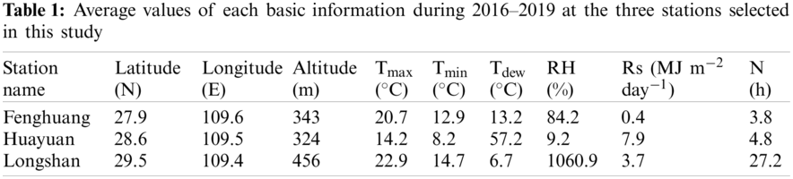
Figure 1: Spatial distributions of the three weather stations used in this study

2.2 Random Forests (RF)

The RF algorithm was proposed by Breiman [45], which was designed and developed using the classification and regression trees (CART) and the concept of “bagging”. The RF algorithm has been widely used in regression and estimation studies. Because it is a machine learning algorithm that can effectively solves high-dimensional regression problems, the RF algorithm can use a subset of the data through bootstrap to process random binary trees. By repeatedly selecting random T (T < N) sample sets, a new training sample set is generated from the N original training samples. In the whole process of selecting samples, the same part of samples may be collected repeatedly. Therefore, a random subset of the training data set needs to be randomly extracted from the original data set for the development and training of the algorithm (the flowchart is shown in Fig. 2). Data sets that are not used in the algorithm are often called out-of-bag data (“out-of-bag” (OOB)). The algorithm's unused data sets will not be used to fit but will be used to test the algorithm's estimation ability.

Figure 2: Flow chart of the RF algorithm

The CART algorithm in the RF algorithm differs from other traditional algorithms, which is based on feature selection according to the Gini coefficient. The criterion for selecting the Gini coefficient is that each child node needs to achieve the highest purity. At this time, the smaller the Gini coefficient, the higher the stability of the algorithm and the higher the purity. CART is a binary tree, which means that each non-leaf node can only produce two branches. If multiple (higher than two) discrete variables are generated on a non-leaf node, the variable may be reused multiple times. Each feature selected from the RF tree is randomly generated from all the features, which reduces the risk of overfitting. Unlike other decision trees, each RF tree is part of the selected feature. Among the selected features in this part, the best feature is selected to divide the left and right subtrees of the decision tree, thereby increasing the randomness and further enhancing the algorithm's generalization ability. Finally, the average of all predictors can be derived.

In short, the final estimation of the RF algorithm is the average of all factors. More detailed information and methods on the RF algorithm can be found in the paper of Breiman [45].

2.3 Categorical Boosting (Catboost)

Gradient boosting on decision trees with categorical features support (such as CatBoost) is a new gradient enhanced decision tree (GBDT) algorithm. The traditional algorithm is pre-processed during the training process, while the CatBoost algorithm performs classification feature processing. Moreover, it can successfully handle classification features. Therefore, compared to the conventional GBDT algorithm, the CatBoost algorithm has more advantages. Specifically, for each example, the CatBoost algorithm randomly arranges and combines the data sets and calculates the average label value of the sample, which is the same as the replacement category value before the given category value.

If a permutation is θ=[σ1,…,σn]nT, it is substituted with:

xσp,k=∑j=1p−1[xσj,k=xσp,k]⋅Yσj+β⋅P∑j=1p−1[xσj,k=xσp,k]+β(1)

where P is a prior value and β is the weight of the prior.

Another advantage of this algorithm is that it uses a new algorithm to calculate the leaf value when selecting the tree structure, which helps reduce the problem of overfitting [42]. The CatBoost algorithm can combine all classification features as a new classification feature. The CatBoost algorithm will recombine it for extensive use when constructing a new segmentation for the tree. Another advantage of the CatBoost algorithm is that it uses the forget tree as a predictor. In addition, the length of each leaf index of the tree is equal to the binary vector of the tree depth. This makes the CatBoost algorithm widely used. First of all, all the floating-point number features, statistical features, and single-hot encoding features are binarized, which are used to calculate the algorithm prediction.

Usually, the prediction offset is the main problem that plagues modeling. In each iteration of GDBT, the loss function uses the same data set to obtain the gradient of the algorithm, and then trains to obtain a basic learner, which will cause the gradient estimation deviation, which will lead to the problem of overfitting the algorithm. The CatBoost algorithm uses ordered boosting to replace gradient estimation in traditional algorithms, reducing gradient estimation bias and improving algorithm capabilities [42]. The structural flow chart of the CatBoost algorithm is shown in Fig. 3, with more detailed information and methods related to the RF algorithm, which can be found in the research of Dorogush et al. [42].

Figure 3: Flow chart of the CatBoost algorithm

The main parameters of both algorithms were optimized using the grid search method. The best performing parameters were used for model training and testing. The main parameters of the RF algorithm are the maximum depth and the number of trees. Trees are more prone to be overfitting if they have larger maximum depths. In this study, the upper and lower limits on the parameters were first determined by trial and error methods. A grid was then created and the best combination of parameters was found by setting different step sizes. CatBoost is also a tree-based algorithm. Although it has many parameters, the main parameters affecting model's accuracy and stability are the same as RF.

2.4 Algorithm Comparison and Statistical Analysis

In this study, four commonly used statistical indicators were selected to analyze and compare the algorithm performance in Tdew estimation under two input scenarios. These statistical indicators were coefficient of determination (R2), root mean square error (RMSE), mean absolute error (MAE) and normalized root mean square error (NRMSE). The mathematical equations of each statistical indicator are described as follows:

R2=[∑i=1n(Oi,m−O¯i,m)(Oi,e−O¯i,e)]2∑i=1n(Oi,m−O¯i,m)2∑i=1n(Oi,e−O¯i,e)2(2)

RMSE=1n∑i=1n(Oi,m−Oi,e)2(3)

MAE=1n∑i=1n|Oi,m−Oi,e|(4)

NRMSE=1n∑i=1n(Oi,m−Oi,e)2O¯i,m(5)

where Oi,m, Oi,e, O¯i,m, O¯i,e and n are the measured, estimated, mean of measured, mean of estimated Tdew and the number of observations, respectively. The higher the R2 value, that is, the closer it is to 1, the higher the accuracy and the better the regression line matches the data. In contrast, algorithm performance is inversely related to RMSE, MAE, and NRMSE.

3  Results and Discussion

3.1 Comparison of Algorithm Accuracy under Various Local Input Combinations

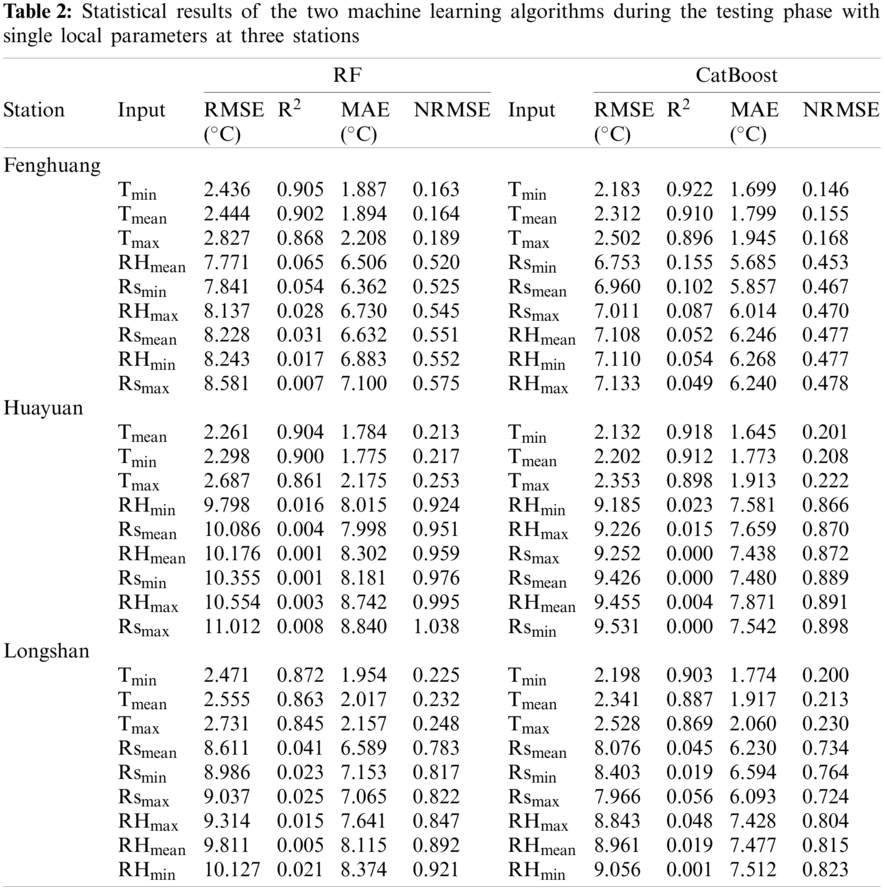
This section evaluates the applicability of RF and CatBoost algorithms for estimating Tdew under the local input scenario, using meteorological data from Fenghuang, Huayuan and Longshan stations in China. The daily meteorological data were maximum, minimum and average temperature (Tmax, Tmin and Tmean), maximum, minimum and average relative humidity (RHmax, RHmin and RHmean), maximum, minimum and average global solar radiation (Rsmax, Rsmin and Rsmean). Table 2 presents the statistical results of the RF and CatBoost algorithms in estimating Tdew during the testing phase at the three stations under nine single-parameter inputs. Overall, the CatBoost algorithm (on average RMSE = 6.304°C and R2 = 0.328) had better performance than the RF algorithm (on average RMSE = 7.014°C and R2 = 0.307). It can be seen from Table 2 that the most relevant parameters for estimating Tdew in Fenghuang, Huayuan and Longshan stations were Tmin, Tmean and Tmin, respectively. The importance of T (on average RMSE = 2.415°C and R2 = 0.891) was greater than that of RH (on average RMSE = 8.889°C and R2 = 0.024) and Rs (on average RMSE = 8.673°C and R2 = 0.038). Therefore, T was the most effective meteorological variable among the single factors, and the estimation accuracy and stability of the CatBoost algorithm were better than those of the RF algorithm.

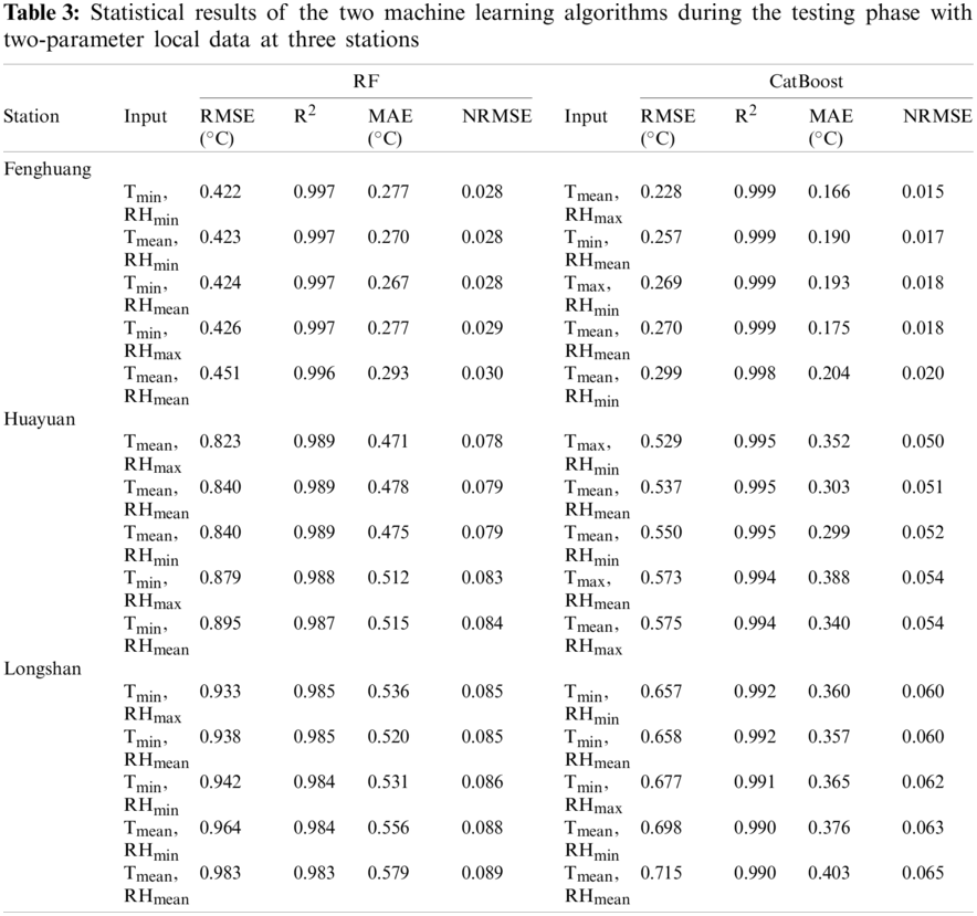
To explore the effect of the two-parameter input combination on Tdew estimation, we randomly combined nine single parameters and determined the top five accurate algorithms with the two parameter inputs. The statistical results during the testing phase are shown in Table 3. It can be seen from Table 3 that under the two-parameter combinations, the CatBoost algorithm (on average RMSE = 0.499°C and R2 = 0.995) had slightly better performance than the RF algorithm (on average RMSE = 0.746°C and R2 = 0.990). When the input parameters were T and RH, the estimation accuracy of each algorithm was highest, which were the most effective meteorological factors under the two-parameter combinations. At Fenghuang station, the optimal parameter combinations of the RF and CatBoost algorithms were Tmin, RHmin (RMSE = 0.422°C and R2 = 0.997) and Tmean, RHmax (RMSE = 0.228°C and R2 = 0.999), respectively. In terms of accuracy, the difference between the CatBoost algorithm and the RF algorithm was small, but the former was more stable than the latter. The performance of the algorithms at different stations was also different. The performance of CatBoost algorithm at Fenghuang station (RMSE = 0.270°C and R2 = 0.999) was better than that at Huayuan (RMSE = 0.537°C and R2 = 0.995) and Longshan (RMSE = 0.715°C and R2 = 0.990) stations when the input combination was Tmean and RHmean. Therefore, the station's geographic location, terrain and climate also affected the accuracy of the algorithm's performance in estimating Tdew. Fan et al. [46] and Feng et al. [37] also confirmed that climate and geographical conditions would significantly impact the algorithm's performance. Under this input combination of Tmean and RHmean, the algorithm's performance was good. Therefore, in terms of two-parameter combination, T and RH were the most effective meteorological factors. Under the parameter combination of Tmean and RHmean, the estimation accuracy and stability of the CatBoost algorithm were better than those of the RF algorithm.

To evaluate the effect of the three-parameter combination on Tdew estimation, we randomly combined nine single parameters and determined the top five accurate algorithms. The statistical results during the testing phase are shown in Table 4. Tables 3 and 4 showed that the trends were almost the same. The CatBoost algorithm was slightly better than the RF algorithm in estimating Tdew (on average RMSE decreased by 40.3%, R2 increased by 0.6%, MAE decreased by 34.7% and NRMSE decreased by 40.6%). The two algorithms were best applied at Fenghuang station, both outperforming the other two stations. The RF and Catboost algorithms had some differences in parameter combinations. The parameter combination contained T and RH in the RF algorithm, while the CatBoost algorithm had a combination of T, RH and Rs. Therefore, T and RH were still the most effective meteorological factors. Algorithms with Tmean and RHmean generally had better stability. In terms of MAE at the Longshan station, the RF and CatBoost algorithms were overfitted and seriously overestimated Tdew (on average MAE = 0.535°C and 0.358°C, respectively). This conclusion was consistent with that obtained by Shiri [29] when estimating daily Tdew using the RF algorithm, which suffered from over-fitting. In the study of Fan et al. [34] for estimating ET0 through a machine learning algorithm, the RF algorithm had a poor-fitting effect relative to the GBDT algorithm. In terms of the three parameters, T and RH were still the most effective meteorological factors for estimating Tdew. The parameter combination of Tmean and RHmean had relatively good accuracy. The estimation accuracy and stability of the CatBoost algorithm were better than those of the RF algorithm.

To better compare the effect of each parameter combination on Tdew estimation, we plotted the estimated Tdew and measured values of some parameter combinations during the testing phase in Fig. 4 (with the CatBoost algorithm at Fenghuang station as an example). It can be seen from Fig. 4 that when the input combination was any single parameter (especially the meteorological factors RHmean, RHmax, RHmin), the scatter diagram had no clear trends, and the scatter was distributed on both sides of the standard line, showing poor accuracy. Adding RH or Rs to T, the algorithm accuracy was significantly improved compared with the single parameter algorithm. Under two- and three-parameter combinations, the scatter points obtained by the algorithm were closer to the standard line and more uniformly distributed when the single parameter was used. It showed that in the study of estimating daily Tdew, the increase of meteorological parameters could improve the estimation performance of the algorithm. Dong et al. [47] also confirmed that the increase in effective meteorological parameters could improve the algorithm's estimation accuracy. However, the difference in accuracy between the two and three-parameter combinations was not significant. It can be seen that the most effective meteorological variables were T and RH. The additional incorporation of Rs to the algorithm failed to improve the algorithm accuracy, and some even declined. It indicated that the Rs was not a necessary parameter to estimate Tdew. Dong et al. [25] also showed that adding extra parameters would reduce the estimation accuracy of the algorithm.

Figure 4: Scatter plots of the daily Tdew estimated by the algorithm and the corresponding measured values during the testing phase under local data input conditions (note: fine line is the best-fitted line)

To better compare the performance of the two algorithms, Fig. 5 compares the statistical results obtained by combining some parameters of the two algorithms during the testing phase at the Fenghuang station. Because the three- and two-parameter combinations of the two algorithms had very similar performances, the single- and two-parameter combinations were compared. It can be seen from the figure that the performance of the RF and CatBoost algorithms was very close. Still, the CatBoost algorithm was slightly better than the RF algorithm under various combinations. For the single-parameter combination, T was more important than RH and Rs. Therefore, the performance of the algorithm with only T data was slightly worse than that of algorithms with two parameters. The required meteorological data was also smallest, which showed the advantage of this input combination. The RMSE values of the two-parameter algorithms were close to 0, showing extremely high stability. Regarding MAE values, algorithms with the single-parameter Rs (on average MAE = 6.275°C) or RH (on average MAE = 6.275°C) showed overfitting. In the RF algorithm, the performance of the input combination of Tmean and RHmin was better than that with RHmin (RMSE decreased by 94.5%, R2 increased by 5758.2%, MAE decreased by 95.7% and NRMSE decreased by 94.6%). It showed that increasing the input number of meteorological parameters effectively improved the estimation accuracy of the algorithm. This conclusion was consistent with previous studies. Therefore, the meteorological factors T and RH were the most influential parameters for estimating Tdew, and the CatBoost algorithm had better performance than the RF algorithm.

Figure 5: Radar chart of the statistical restuls during the testing phase under local input conditions at the Fenghuang station

3.2 Comparing Algorithm Accuracy by Replacing Local Data with Cross-Station Data

It is important to use meteorological data from cross stations in different regions to estimate Tdew at the target station. In some developing countries with incomplete measurement equipment, some meteorological data cannot be obtained normally due to various reasons. Therefore, it is necessary to use this method for Tdew estimation. The method also reflected the modeling ability of the regional application of the algorithm [37]. This section evaluated the applicability of RF and CatBoost algorithms to estimate the target-station Tdew using meteorological data from cross stations during the testing phase. Daily meteorological data at Fenghuang (Fh), Huayuan (Hy) and Longshan (Ls) stations (different regions) in China were used. The daily meteorological data were maximum, minimum and average temperature (Tmax, Tmin and Tmean), maximum, minimum and average relative humidity (RHmax, RHmin and RHmean), maximum, minimum and average global solar radiation (Rsmax, Rsmin and Rsmean). For example, Fh-Hy meant that the meteorological data of Huayuan station were applied to Fenghuang station, and so on. To explore the effect of the two-parameter combination on Tdew after the station exchange, we randomly combined nine single parameters and explored the top five accurate algorithms. The statistical results during the testing phase are shown in Table 5. It can be seen from Table 5 that the performance of most CatBoost algorithms was better than that of RF algorithms. Except for the parameter combination of Tmean and RHmax in Fh-Hy and Fh-Ls, the performance of the CatBoost algorithm was poor (on average RMSE = 0.512°C, R2 = 0.914, MAE = 1.820°C and NRMSE = 0.212). On the whole, before and after the station change, the best five parameter combinations did not change at each station, but the performance order changed. For example, the best two-parameter combination of the CatBoost algorithm at Fenghuang station before the change was Tmean, RHmax (RMSE = 0.228°C, R2 = 0.999, MAE = 0.166°C and NRMSE = 0.015). The best two-parameter combination after the station change was Tmin, RHmean (RMSE = 0.307°C, R2 = 0.998, MAE = 0.224°C and NRMSE = 0.028). The performance difference of each parameter combination was small, which further confirmed that the CatBoost algorithm had high stability. In Fh-Ls, the optimal parameter combination of the RF algorithm before switching stations was Tmin, RHmin. The ranking remained unchanged after switching stations, and RMSE was decreased by 12.8%. It showed that in Fh-Ls, when the input parameter combination was Tmin, RHmin, the algorithm had higher stability and the stability was improved after the station was changed. The feasibility of using the meteorological data from cross stations to estimate the target-station Tdew was confirmed. In Ls-Hy, the overall RMSE of the CatBoost algorithm was less than that of the RF algorithm, and the R2 was greater than that of the RF algorithm. The accuracy and stability of the CatBoost algorithm after station replacement were better than those of the RF algorithm. This conclusion was also consistent with the finding of Lu et al. [39]. However, compared with the algorithm without station exchange, the CatBoost (on average RMSE increased by 39.5%, R2 decreased by 0.6%) and RF (on average RMSE increased by 29.3%, R2 decreased by 1.0%) algorithms lowered the performance. It showed that the application of data from Huayuan station instead of Longshan station had instability, but other applications of station exchange had good stability.

To explore the impact of the three-parameter combination on Tdew after the station exchange, we randomly combined nine single parameters and determined the top five accurate algorithms. The statistical results during the test period are shown in Table 6. Overall, the performance of the CatBoost algorithm was slightly better than that of the RF algorithm in most cases. Consistent with the trends in Table 5, before and after the station exchange, the top five parameter combinations did not change. Only the performance order changed, indicating that the two algorithms had certain stability in Tdew estimation. In Fh-Hy, the RF algorithm's performance after the exchange was improved compared to the that before the exchange (on average RMSE decreased by 22.5%, R2 increased by 1.0%). In contrast, the performance of the CatBoost algorithm was slightly reduced (on average RMSE increased by 49.2%, R2 decreased by 0.1%). The RF algorithm's estimation performance was slightly better than that of the CatBoost algorithm, indicating that the RF algorithm was more suitable for Fh-Hy and the station replacement may also effectively improve the algorithm performance. After changing stations, when the parameter combination was Tmean, RHmin, Rsmean, the performance of the RF algorithm was best (RMSE = 0.292°C, R2 = 1.000, MAE = 0.221°C and NRMSE = 0.026). In Ls-Hy, the CatBoost algorithm (on average RMSE = 0.810°C and R2 = 0.989) was better than the RF algorithm (on average RMSE = 1.198°C and R2 = 0.976). However, compared with the Longshan station before the exchange, the performance of RF (on average RMSE increased by 28.3%, R2 decreased by 0.8%) and CatBoost algorithm (on average RMSE increased by 41.2%, R2 decreased by 0.5%) were both reduced. It showed that the meteorological data of Huayuan Station could not be applied to Longshan Station, consistent with the performance of each algorithm of the two-parameter combinations. However, in the processing of other station exchanges, each algorithm showed good performance, confirming the feasibility of using the meteorological data of cross stations for Tdew estimation. It can be known from the three-parameter combinations that both had meteorological factors of T and RH. It showed that T and RH were the most effective meteorological factors for estimating Tdew, which was highly consistent with the conclusions of Mehdizadeh et al. [37]. Rs was more suitable for the CatBoost algorithm at Huayuan and Longshan stations.

Figure 6: Scatter plots of the daily Tdew estimated by the algorithm and the corresponding measured values during the testing phase using cross-station data

To better compare each algorithm's impact to estimate Tdew at the target station using meteorological data from cross stations. We plotted estimated Tdew of some parameter combinations and measured Tdew during the test period in the case of station exchange and draw it in Fig. 6 (using Fh-Hy as an example). Fig. 6 showed that the performance of each algorithm in the case of two- and three-parameter combinations after the station exchange was very close. The difference in estimation accuracy was small, and the resulting scattered points were evenly distributed, all very close to the standard line. It showed that in the case of changing stations, the combination of T and RH parameters achieved high accuracy. Increasing the number of parameters made the algorithm more stable, but there were also a small number of algorithms with reduced accuracy. The CatBoost algorithm was slightly better than the RF algorithm. When the input parameter combination was Tmean, RHmean, the estimation accuracy of the CatBoost algorithm (R2 = 0.998) was slightly better than that of the RF algorithm (R2 = 0.995). Fig. 7 showed the distribution of the RMSE values of each algorithm in Tables 5 and 6 after each station exchange into a bar graph. As shown in Fig. 7, the CatBoost algorithm was more stable than the RF algorithm, and the distribution was more uniform. Among them, the stability of the algorithm was the most uniform under the conditions of Hy-Fh, Hy-Ls and Ls-Hy. The highest stability was obtained by the CatBoost algorithm in the case of Fh-Hy and Fh-Ls. The worst stability was found in the RF algorithm in the case of Ls-Hy (on average RMSE > 1.1°C). The comprehensive description confirmed the feasibility of using the meteorological data from cross stations to estimate Tdew at the target station. Each algorithm had good performance. It also showed that the modeling ability of the regional application of the algorithm had great potential. However, the CatBoost algorithm performed better than the RF algorithm and was more suitable for regional application in estimating daily Tdew. The best parameter combination was the two-parameter combination of T and RH, which had the highest cost performance.

Figure 7: The RMSE distribution of the two algorithms after changing stations

3.3 Comprehensive Comparison of the Algorithm with Local Input and Cross-Station Input

Tables 7 and 8 show the average statistical results of the first five parameter combinations obtained when each algorithm using local and cross-station input data in the case of two-parameter and three-parameter combinations, respectively. It can be seen from Table 7 that in the two-parameter combinations, the CatBoost algorithm (on average RMSE = 0.568°C, R2 = 0.990, MAE = 0.407°C and NRMSE = 0.056) was better than the RF algorithm (on average RMSE = 0.739°C, R2 = 0.989, MAE = 0.432°C and NRMSE = 0.063). In Ls-Hy, each algorithm showed poor performance. Conversely, the best performance of each algorithm at Fh-Ls was better than the performance of the algorithms with local inputs. This indicated the feasibility of estimating daily Tdew at the target station using data from cross stations in different regions. This also provided the possibility in some developing countries to obtain unmeasured Tdew through regional modeling. As concluded by Shiri et al. [20]. They selected ANN and GEP algorithms for cross-station processing at two stations, Incheon and Seoul, Korea, to estimate Tdew values. The research provides guidance for regionalized modeling in Korea. As shown in Table 7, the average RMSE of the RF and CatBoost algorithms varied from 0.415 to 1.231°C and 0.265 to 0.950°C. It can be seen that the CatBoost algorithm was also superior to the RF algorithm in terms of instability. Tables 7 and 8 had very similar trends. In the three-parameter combinations, the average RMSE of RF and CatBoost algorithms ranged from 0.331 to 1.198°C and 0.246 to 0.810°C. The three-parameter combinations had higher stability than the two-parameter combinations, which was also consistent with the conclusions above. Under the combination of the three parameters of the local and cross-station inputs, the CatBoost algorithm exhibited the best accuracy and stability at Fenghuang station (on average RMSE = 0.315°C and R2 = 0.998).

Fig. 8 shows the average statistical values corresponding to each algorithm. As can be seen in Fig. 8, the three-parameter combinations were more stable. Because there were many parameters in the three-parameter combinations, the algorithm's performance to estimate Tdew was more stable. Still, the accuracy of each algorithm under the two-parameter and three-parameter combinations was not much different. Combining the data in Tables 2–6, adding meteorological parameters could improve the estimation accuracy of the algorithm, but adding extra parameters would also reduce the accuracy of the algorithm in estimating Tdew. This result also confirmed the previous conclusions. From another point of view, the correct choice of parameters is very important. Moreover, the experience of the scholar determines the amount of work involved in the research [48–50]. In Fig. 8, the average statistical results in the CatBoost algorithm varied more than the RF algorithm. For example, in Fh-Ls, the average MAE of the CatBoost algorithm was decreased by 58.1%, and the stability of the algorithm was improved under the three-parameter combinations. The estimation accuracy and stability of the CatBoost algorithm were better than the RF algorithm at the corresponding stations. The CatBoost algorithm was more suitable for regional application in estimating Tdew.

To better illustrate the importance of each meteorological factor in estimating Tdew, we have plotted the number of occurrences of each meteorological factor listed in Tables 2–6 in Fig. 9. The most frequently occurring meteorological factors in the RF algorithm were Tmin (54 times) and RHmin (54 times). The most frequently occurring meteorological factor in the CatBoost algorithm were Tmin (51 times), followed by RHmean (45 times). According to the parameter combinations in Tables 2–6, Rs were rarely present under the three-parameter combinations. It can be seen that the meteorological factors T and RH were the most effective parameters. This result was consistent with the previous conclusion. Moreover, the meteorological factors T and RH were better obtained than Rs, which was also the advantage of choosing the combination algorithm of factors T and RH, which was consistent with the conclusion of Dong et al. [47,51]. Rs can be used as an alternative parameter to estimate Tdew. It can be seen from Table 8 that the minimum values and average values appeared more frequently in the meteorological factors T and RH. This reason may be because, in daily meteorological data changes, the minimum values and average values were closer to the values, while the maximum values deviated larger. Mehdizadeh et al. [38] also discovered this scenario. Moreover, the data processing speed of the CatBoost algorithm was better than that of the RF algorithm. The calculation CPU time required of both the CatBoost and RF algorithms was less than 1 s. The CatBoost algorithm has a very small advantage over the RF algorithm, which was also consistent with the results of Huang et al. [52]. The accuracy and stability of each algorithm in estimating Tdew were based on the performance of scatter plots, radar charts, bar charts, and line charts. As a result, the CatBoost algorithm was the best and the most effective meteorological factors for the two input scenarios were T and RH. The most cost-effective parameter combination was the two-parameter combination of T and RH. For both algorithms, it was feasible to estimate Tdew at the target station using different regions’ cross-station data. This conclusion also confirmed the modeling and estimation capabilities of the regional application of the algorithm.

Figure 8: Percentage growth in statistical results of the two algorithms of the three-parameter combinations under local and cross-station scenarios relative to the average statistical indicators under the two-parameter combinations

Figure 9: The number of occurrences of each parameter in all listed parameter combinations

4  Conclusions

This paper evaluated the applicability of a new algorithm (CatBoost) under two input scenarios (local and cross-station data) combined with limited meteorological data from different regional stations in China to accurately estimate daily Tdew and extend it to regional applications. The RF algorithm was also assessed for comparison. The daily routine meteorological data (including Tmax, Tmin, Tmean, RHmax, RHmin, RHmean, Rsmax, Rsmin and Rsmean) at three weather stations of Hunan from 2016 to 2019 were used to train and test the algorithms. The results showed that in the absence of complete meteorological parameters (with meteorological factor T), each machine learning algorithm achieved satisfactory estimation accuracy at the target station. During the testing phase of the two-input scenarios, the CatBoost algorithm was better than the RF algorithm. The accuracy and stability of most machine learning algorithms were positively correlated with the number of input parameters, and the performance of the algorithm was significantly better than that of the single-parameter when the two parameters were used as inputs. The algorithm performance difference was minuscule when two and three parameters were used as inputs. The top five accurate algorithms of the two-parameter combinations included T and RH, whose importance were greater than that of Rs, and the meteorological data were easier to obtain relative to Rs. The main meteorological factors were the minimum and average T and RH. Incorporation of Rs when estimating Tdew may reduce the algorithm performance. Therefore, the increase of parameters sometimes caused the increase of influencing factors, so that the performance of the algorithm may decline. When normal meteorological data are partially or wholly lacking in certain areas, meteorological data from cross-stations in different regions can be used to form various combinations of parameters as input to estimate Tdew at the target station. This conclusion confirmed the potential of both algorithms to extend local modeling to regional applications. Considering factors such as accuracy and stability, the CatBoost algorithm implemented regional modeling in China and even similar climate regions worldwide and estimates that Tdew had excellent potential. The most practical input parameter combination in the two input scenarios were T and RH. Differences in the study area and climate will also lead to different regional applicability of the algorithm and incomplete meteorological data. Some new hybrid machine learning algorithms have also been developed to obtain higher accuracy in estimating Tdew.

Acknowledgement: This study was jointly supported by the Shandong Provincial Natural Science Fund (ZR2020ME254 and ZR2020QD061). Thanks to the National Meteorological Information Center of China Meteorological Administration for offering the meteorological data.

Funding Statement: This research was supported by the Shandong Provincial Natural Science Fund (ZR2020ME254 and ZR2020QD061).

Conflicts of Interest: The authors declare that they have no conflicts of interest to report regarding the present study.

References

 1.  Blanco, J. M., Pena, F. (2008). Increase in the boiler's performance in terms of the acid dew point temperature: Environmental advantages of replacing fuels. Applied Thermal Engineering, 28(7), 777–784. DOI 10.1016/j.applthermaleng.2007.06.024. [Google Scholar] [CrossRef]

 2.  Jradi, M., Riffat, S. (2014). Experimental and numerical investigation of a dew-point cooling system for thermal comfort in buildings. Applied Energy, 132, 524–535. DOI 10.1016/j.apenergy.2014.07.040. [Google Scholar] [CrossRef]

 3.  Yang, Y., Ren, C., Yang, C., Tu, M., Luo, B. et al. (2021). Energy and exergy performance comparison of conventional, dew point and new external-cooling indirect evaporative coolers. Energy Conversion and Management, 230, 113824. DOI 10.1016/j.enconman.2021.113824. [Google Scholar] [CrossRef]

 4.  Ali, M., Ahmad, W., Sheikh, N. A., Ali, H., Kousar, R. et al. (2021). Performance enhancement of a cross flow dew point indirect evaporative cooler with circular finned channel geometry. Journal of Building Engineering, 35, 101980. DOI 10.1016/j.jobe.2020.101980. [Google Scholar] [CrossRef]

 5.  Robinson, P. J. (2000). Temporal trends in United States dew point temperatures. International Journal of Climatology, 20(9), 985–1002. DOI 10.1002/1097-0088(200007)20:9&<985::AID-JOC513>3.0.CO;2-W. [Google Scholar] [CrossRef]

 6.  Kim, S., Singh, V. P., Lee, C., Seo, Y. (2015). Modeling the physical dynamics of daily dew point temperature using soft computing techniques. Journal of Civil Engineering, 19(6), 1930–1940. DOI 10.1007/s12205-014-1197-4. [Google Scholar] [CrossRef]

 7.  Lawrence, M. G. (2005). The relationship between relative humidity and the dewpoint temperature in moist air: A simple conversion and applications. Bulletin of the American Meteorological Society, 86(2), 225–234. DOI 10.1175/BAMS-86-2-225. [Google Scholar] [CrossRef]

 8.  Drezner, T. D. (2007). An analysis of winter temperature and dew point under the canopy of a common sonoran desert nurse and the implications for positive plant interactions. Journal of Arid Environments, 69(4), 554–568. DOI 10.1016/j.jaridenv.2006.11.003. [Google Scholar] [CrossRef]

 9.  Hubbard, K. G., Mahmood, R., Carlson, C. (2003). Estimating daily dew point temperature for the northern great plains using maximum and minimum temperature. Agronomy Journal, 95(2), 323–328. DOI 10.2134/agronj2003.3230. [Google Scholar] [CrossRef]

10. Sandstrom, M. A., Lauritsen, R. G., Changnon, D. (2004). A central-US summer extreme dew-point climatology (1949–2000). Physical Geography, 25(3), 191–207. DOI 10.2747/0272-3646.25.3.191. [Google Scholar] [CrossRef]

11. Parlange, M. B., Katz, R. W. (2000). An extended version of the richardson model for simulating daily weather variables. Journal of Applied Meteorology, 39(5), 610–622. DOI 10.1175/1520-0450-39.5.610. [Google Scholar] [CrossRef]

12. Hou, J., Huang, C., Zhang, Y., Guo, J. (2020). On the value of available MODIS and landsat8 OLI image pairs for MODIS fractional snow cover mapping based on an artificial neural network. IEEE Transactions on Geoscience and Remote Sensing, 58(6), 4319–4334. DOI 10.1109/TGRS.2019.2963075. [Google Scholar] [CrossRef]

13. Kuter, S., Akyurek, Z., Weber, G. (2018). Retrieval of fractional snow covered area from MODIS data by multivariate adaptive regression splines. Remote Sensing of Environment, 205, 236–252. DOI 10.1016/j.rse.2017.11.021. [Google Scholar] [CrossRef]

14. Kuter, S. (2021). Completing the machine learning saga in fractional snow cover estimation from MODIS terra reflectance data: Random forests versus support vector regression. Remote Sensing of Environment, 255, 112294. DOI 10.1016/j.rse.2021.112294. [Google Scholar] [CrossRef]

15. Houborg, R., McCabe, M. F. (2018). A hybrid training approach for leaf area index estimation via cubist and random forests machine-learning. ISPRS Journal of Photogrammetry and Remote Sensing, 135, 173–188. DOI 10.1016/j.isprsjprs.2017.10.004. [Google Scholar] [CrossRef]

16. Czyzowska-Wisniewski, E. H., van Leeuwen, W. J., Hirschboeck, K. K., Marsh, S. E., Wisniewski, W. T. (2015). Fractional snow cover estimation in complex alpine-forested environments using an artificial neural network. Remote Sensing of Environment, 156, 403–417. DOI 10.1016/j.rse.2014.09.026. [Google Scholar] [CrossRef]

17. García-Gutiérrez, J., Mateos-García, D., Garcia, M., Riquelme-Santos, J. C. (2015). An evolutionary-weighted majority voting and support vector machines applied to contextual classification of LiDAR and imagery data fusion. Neurocomputing, 163, 17–24. DOI 10.1016/j.neucom.2014.08.086. [Google Scholar] [CrossRef]

18. Shank, D. B., Hoogenboom, G., McClendon, R. W. (2008). Dewpoint temperature prediction using artificial neural networks. Journal of Applied Meteorology and Climatology, 47(6), 1757–1769. DOI 10.1175/2007JAMC1693.1. [Google Scholar] [CrossRef]

19. Zounemat-Kermani, M. (2012). Hourly predictive levenberg–Marquardt ANN and multi linear regression models for predicting of dew point temperature. Meteorology and Atmospheric Physics, 117(3), 181–192. DOI 10.1007/s00703-012-0192-x. [Google Scholar] [CrossRef]

20. Shiri, J., Kim, S., Kisi, O. (2014). Estimation of daily dew point temperature using genetic programming and neural networks approaches. Hydrology Research, 45(2), 165–181. DOI 10.2166/nh.2013.229. [Google Scholar] [CrossRef]

21. Nadig, K., Potter, W., Hoogenboom, G., McClendon, R. (2013). Comparison of individual and combined ANN models for prediction of air and dew point temperature. Applied Intelligence, 39(2), 354–366. DOI 10.1007/s10489-012-0417-1. [Google Scholar] [CrossRef]

22. Mohammadi, K., Shamshirband, S., Petković, D., Yee, L., Mansor, Z. (2016). Using ANFIS for selection of more relevant parameters to predict dew point temperature. Applied Thermal Engineering, 96, 311–319. DOI 10.1016/j.applthermaleng.2015.11.081. [Google Scholar] [CrossRef]

23. Kisi, O., Kim, S., Shiri, J. (2013). Estimation of dew point temperature using neuro-fuzzy and neural network techniques. Theoretical and Applied Climatology, 114(3), 365–373. DOI 10.1007/s00704-013-0845-9. [Google Scholar] [CrossRef]

24. Baghban, A., Bahadori, M., Rozyn, J., Lee, M., Abbas, A. et al. (2016). Estimation of air dew point temperature using computational intelligence schemes. Applied Thermal Engineering, 93, 1043–1052. DOI 10.1016/j.applthermaleng.2015.10.056. [Google Scholar] [CrossRef]

25. Dong, J., Wu, L., Liu, X., Fan, C., Leng, M. et al. (2020). Simulation of daily diffuse solar radiation based on three machine learning models. Computer Modeling in Engineering & Sciences, 123(1), 49–73. DOI 10.32604/cmes.2020.09014. [Google Scholar] [CrossRef]

26. Wu, L., Fan, J. (2019). Comparison of neuron-based, kernel-based, tree-based and curve-based machine learning models for predicting daily reference evapotranspiration. PLoS One, 14(5), e217520. DOI 10.1371/journal.pone.0217520. [Google Scholar] [CrossRef]

27. Han, Y., Wu, J., Zhai, B., Pan, Y., Huang, G. et al. (2019). Coupling a bat algorithm with xgboost to estimate reference evapotranspiration in the arid and semiarid regions of China. Advances in Meteorology, 2019, 9575782. DOI 10.1155/2019/9575782. [Google Scholar] [CrossRef]

28. Wu, L., Huang, G., Fan, J., Zhang, F., Wang, X. et al. (2019). Potential of kernel-based nonlinear extension of arps decline model and gradient boosting with categorical features support for predicting daily global solar radiation in humid regions. Energy Conversion and Management, 183, 280–295. DOI 10.1016/j.enconman.2018.12.103. [Google Scholar] [CrossRef]

29. Shiri, J. (2019). Prediction vs. estimation of dewpoint temperature: Assessing GEP, MARS and RF models. Hydrology Research, 50(2), 633–643. DOI 10.2166/nh.2018.104. [Google Scholar] [CrossRef]

30. Attar, N. F., Khalili, K., Behmanesh, J., Khanmohammadi, N. (2018). On the reliability of soft computing methods in the estimation of dew point temperature: The case of arid regions of Iran. Computers and Electronics in Agriculture, 153, 334–346. DOI 10.1016/j.compag.2018.08.029. [Google Scholar] [CrossRef]

31. Mehdizadeh, S., Behmanesh, J., Khalili, K. (2017). Using MARS, SVM, GEP and empirical equations for estimation of monthly mean reference evapotranspiration. Computers and Electronics in Agriculture, 139, 103–114. DOI 10.1016/j.compag.2017.05.002. [Google Scholar] [CrossRef]

32. Deka, P. C., Patil, A. P., Yeswanth Kumar, P., Naganna, S. R. (2018). Estimation of dew point temperature using SVM and ELM for humid and semi-arid regions of India. ISH Journal of Hydraulic Engineering, 24(2), 190–197. DOI 10.1080/09715010.2017.1408037. [Google Scholar] [CrossRef]

33. Amirmojahedi, M., Mohammadi, K., Shamshirband, S., Danesh, A. S., Mostafaeipour, A. et al. (2016). A hybrid computational intelligence method for predicting dew point temperature. Environmental Earth Sciences, 75(5), 415. DOI 10.1007/s12665-015-5135-7. [Google Scholar] [CrossRef]

34. Fan, J., Yue, W., Wu, L., Zhang, F., Cai, H. et al. (2018). Evaluation of SVM, ELM and four tree-based ensemble models for predicting daily reference evapotranspiration using limited meteorological data in different climates of China. Agricultural and Forest Meteorology, 263, 225–241. DOI 10.1016/j.agrformet.2018.08.019. [Google Scholar] [CrossRef]

35. Wong, P. K., Wong, K. I., Vong, C. M., Cheung, C. S. (2015). Modeling and optimization of biodiesel engine performance using kernel-based extreme learning machine and cuckoo search. Renewable Energy, 74, 640–647. DOI 10.1016/j.renene.2014.08.075. [Google Scholar] [CrossRef]

36. Feng, Y., Jia, Y., Cui, N., Zhao, L., Li, C. et al. (2017). Calibration of hargreaves model for reference evapotranspiration estimation in sichuan basin of Southwest China. Agricultural Water Management, 181, 1–9. DOI 10.1016/j.agwat.2016.11.010. [Google Scholar] [CrossRef]

37. Feng, Y., Peng, Y., Cui, N., Gong, D., Zhang, K. (2017). Modeling reference evapotranspiration using extreme learning machine and generalized regression neural network only with temperature data. Computers and Electronics in Agriculture, 136, 71–78. DOI 10.1016/j.compag.2017.01.027. [Google Scholar] [CrossRef]

38. Mehdizadeh, S., Behmanesh, J., Khalili, K. (2017). Application of gene expression programming to predict daily dew point temperature. Applied Thermal Engineering, 112, 1097–1107. DOI 10.1016/j.applthermaleng.2016.10.181. [Google Scholar] [CrossRef]

39. Lu, X., Ju, Y., Wu, L., Fan, J., Zhang, F. et al. (2018). Daily pan evaporation modeling from local and cross-station data using three tree-based machine learning models. Journal of Hydrology, 566, 668–684. DOI 10.1016/j.jhydrol.2018.09.055. [Google Scholar] [CrossRef]

40. Karimi, S., Kisi, O., Kim, S., Nazemi, A. H., Shiri, J. (2017). Modelling daily reference evapotranspiration in humid locations of South Korea using local and cross-station data management scenarios. International Journal of Climatology, 37(7), 3238–3246. DOI 10.1002/joc.4911. [Google Scholar] [CrossRef]

41. Fan, J., Wu, L., Zhang, F., Cai, H., Zeng, W. et al. (2019). Empirical and machine learning models for predicting daily global solar radiation from sunshine duration: A review and case study in China. Renewable and Sustainable Energy Reviews, 100, 186–212. DOI 10.1016/j.rser.2018.10.018. [Google Scholar] [CrossRef]

42. Dorogush, A. V., Ershov, V., Gulin, A. (2018). CatBoost: gradient boosting with categorical features support. Machine Learning, 1–7. https://arxiv.org/abs/1810.11363. [Google Scholar]

43. Aler, R., Galván, I. M., Ruiz-Arias, J. A., Gueymard, C. A. (2017). Improving the separation of direct and diffuse solar radiation components using machine learning by gradient boosting. Solar Energy, 150, 558–569. DOI 10.1016/j.solener.2017.05.018. [Google Scholar] [CrossRef]

44. Fan, J., Wang, X., Wu, L., Zhou, H., Zhang, F. et al. (2018). Comparison of support vector machine and extreme gradient boosting for predicting daily global solar radiation using temperature and precipitation in humid subtropical climates: A case study in China. Energy Conversion and Management, 164, 102–111. DOI 10.1016/j.enconman.2018.02.087. [Google Scholar] [CrossRef]

45. Breiman, L. (2001). Random forests. Machine Learning, 45(1), 5–32. DOI 10.1023/A:1010933404324. [Google Scholar] [CrossRef]

46. Fan, J., Wu, L., Ma, X., Zhou, H., Zhang, F. (2020). Hybrid support vector machines with heuristic algorithms for prediction of daily diffuse solar radiation in air-polluted regions. Renewable Energy, 145, 2034–2045. DOI 10.1016/j.renene.2019.07.104. [Google Scholar] [CrossRef]

47. Dong, J., Wu, L., Liu, X., Li, Z., Gao, Y. et al. (2020). Estimation of daily dew point temperature by using bat algorithm optimization based extreme learning machine. Applied Thermal Engineering, 165, 114569. DOI 10.1016/j.applthermaleng.2019.114569. [Google Scholar] [CrossRef]

48. Owolabi, K. M., Baleanu, D. (2021). Emergent patterns in diffusive Turing-like systems with fractional-order operator. Neural Computing and Applications, 1, 1–18. DOI 10.1007/s00521-021-05917-8. [Google Scholar] [CrossRef]

49. Momigliano, P., Florin, A., Merilä, J. (2021). Biases in demographic modeling affect our understanding of recent divergence. Molecular Biology and Evolution, 38(7), 2967–2985. DOI 10.1093/molbev/msab047. [Google Scholar] [CrossRef]

50. Rybak, I., Schwarzmeier, C., Eggenweiler, E., Rüde, U. (2021). Validation and calibration of coupled porous-medium and free-flow problems using pore-scale resolved models. Computational Geosciences, 25(2), 621–635. DOI 10.1007/s10596-020-09994-x. [Google Scholar] [CrossRef]

51. Dong, J., Liu, X., Huang, G., Fan, J., Wu, L. et al. (2020). Comparison of four bio-inspired algorithms to optimize KNEA for predicting monthly reference evapotranspiration in different climate zones of China. Computers and Electronics in Agriculture, 186, 106211. DOI 10.1016/j.compag.2021.106211. [Google Scholar] [CrossRef]

52. Huang, G., Wu, L., Ma, X., Zhang, W., Fan, J. et al. (2019). Evaluation of CatBoost method for prediction of reference evapotranspiration in humid regions. Journal of Hydrology, 574, 1029–1041. DOI 10.1016/j.jhydrol.2019.04.085. [Google Scholar] [CrossRef]

This work is licensed under a Creative Commons Attribution 4.0 International License, which permits unrestricted use, distribution, and reproduction in any medium, provided the original work is properly cited.