| Computer Modeling in Engineering & Sciences |
DOI: 10.32604/cmes.2022.018665
ARTICLE
Theoretical Investigation of Two-Dimensional Nonlinear Radiative Thermionics in Nano-MHD for Solar Insolation: A Semi-Empirical Approach
1School of Systems and Technology, University of Management and Technology, Lahore, 54000, Pakistan
2Energy Research Centre, COMSATS University Islamabad, Lahore Campus, Lahore, 54000, Pakistan
*Corresponding Author: Usman Inayat. Email: usman.inayat@umt.edu.pk
Received: 09 August 2021; Accepted: 02 September 2021
Abstract: In this contemporary study, theoritical investigation of nanofluidic model is thought-out. Two-dimensional nanomaterials based mixed flow is considered here. Convective solar radiative heat transport properties have been investigated over a nonlinearly stretched wall in the presence of magneto-hydrodynamic (MHD), by innovative application of semi analytical “optimal homotopy asymptotic method (OHAM)”. OHAM does not require any discretization, linearization and small parameter assumption. OHAM describes extremely precise
Keywords: Magneto-hydrodynamic (MHD); OHAM; nanofluid; solar radiative; stretched wall
The most abundance renewable energy source for best alternative to conventional fossil fuel-based generation is solar energy. Electric energy and heat energy can be generated through sun light using photoelectric effect on photovoltaic panels and photothermal conversion on concentrated solar thermal plants, respectively. The increasing rate of solar absorption helps in improving energy output production of both photovoltaic panels and concentrated solar thermal plants. The efficient absorption of solar energy results in reliable use of renewable energy and better conversion into thermal energy, which results in least dependence on fossil fuels. However, the current heat collectors and photovoltaic panels suffer from inefficient sunlight absorption that results in signification energy loss and low efficiency. In this regard, water dispersed nanoparticles are being extensively studied for improving sunlight absorption. Various nanomaterials have been proposed and tested for ameliorating sunlight absorption efficiency. The sunlight absorption capability is improved by using photoactive nanomaterials for polymeric photovoltaic panels. It is known that these polymeric photovoltaic panels absorb photons with bandgap of 2-ev. Therefore, nanomaterials are needed to widen this energy bandgap for absorbing more sunlight. In this regard, a hybrid solar cell was proposed for more solar energy absorption from visible to near-infrared energy band.
The heterojunction photovoltaic cells were examined for analyzing their solar absorption enhancement capability using half-coaxial crystalline silicon nanowire arrays [1]. High bandgap solar cell was integrated with upconverter at its for stronger sunlight absorption in the near infrared region [2]. The broadband absorption enhancement was achieved in Si films by their crystallization in liquid phase on textured glass. The absorption enhancement was increased by 36.3% as compared to planar reference film [3]. A two-dimensional photonic-structured perovskite photovoltaic cell was investigated, which provided 65.7% more absorption efficiency over the visible range [4]. Photonic crystals were placed on the top surface of microcrystalline silicon solar cells to enhance light absorption with the exploitation of resonant effects in photonic crystal. The efficiency was reported to be increased by 11% due to enhanced short circuit current density [5]. The dye-sensitized photovoltaic cells were combined with uncapped lead sulfide nanocrystals to achieve increase in absorption capability by 7.9% [6].
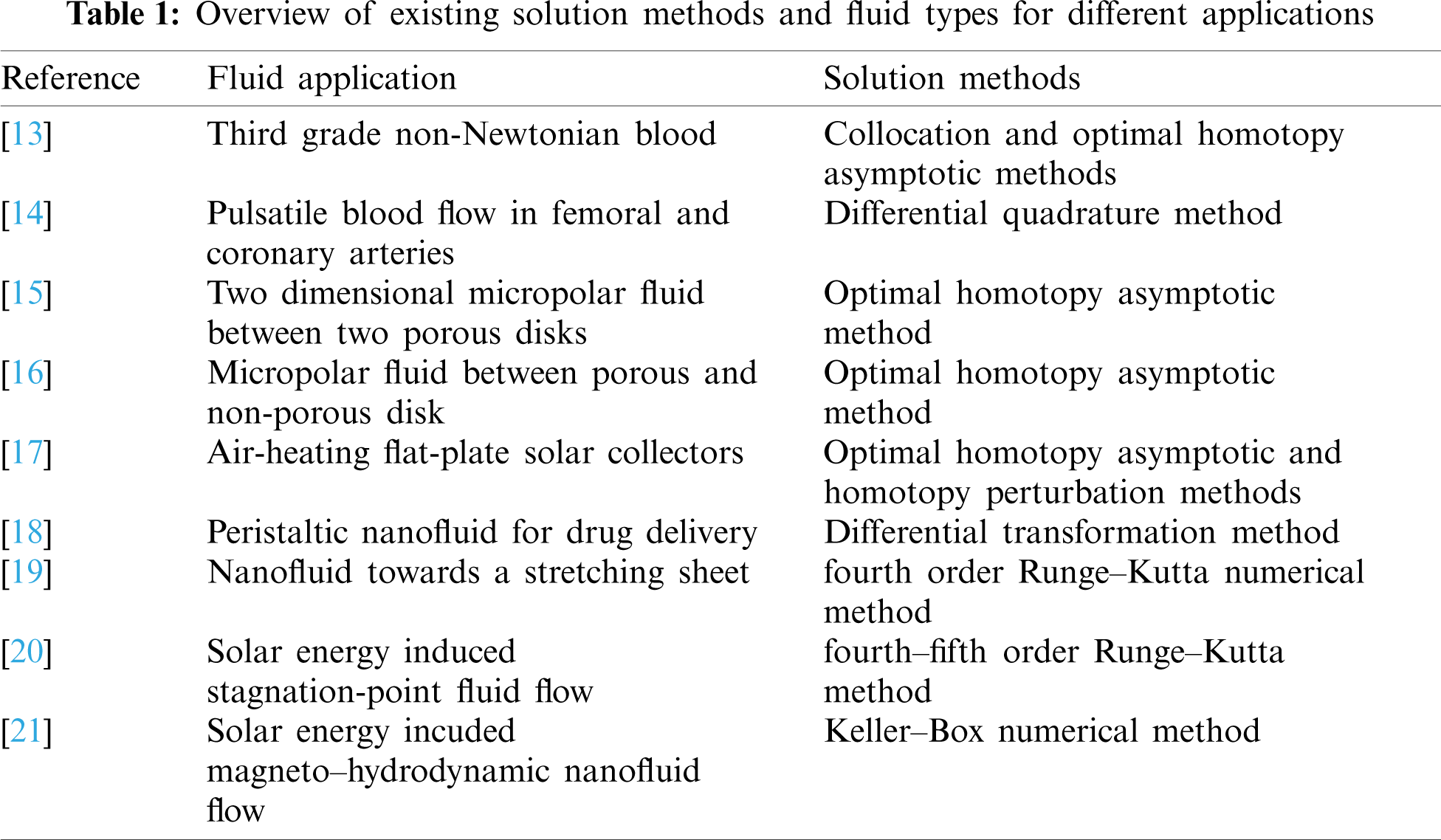
The index-guiding microstructured optical fiber, which is ionic-liquid adorned, were adopted to construct an optical fiber light detector by splicing it with two air holes in innermost layer. It was reported to have power density sensitivity to achieve value of 1.529 dB/(mW.mm2) [7]. The titanium nitride nanoparticles were investigated in water with experimental results to report higher sunlight absorption efficiency as compared to carbon nanoparticles [8]. The surface mounted gold particles based copper-doped TiO2 nanocomposites were synthesized using a facile step method. It was observed that they were able to enhance more visible light spectrum absorption as compared to pure TiO2 and copper-doped TiO2 [9]. The light energy concertation was achieved at mesoscale volumes using light-absorbing nanoparticles contained aqueous solutions. The high efficiency steam was obtained using sunlight even in case of having far below boiling temperature of the bulk fluid [10]. The experimental results were presented to show that the rapid water vaporization with sunlight can be achieved using silicon nanoparticles in water [11]. Rapid sunlight to heat conversion was achieved using plasmonic nanocomposites with filler concentration at volumetric ppm level [12]. Collocation and optimal homotopy asymptotic methods had been used for investigation of third grade non-Newtonian blood fluid [13]. Similarly, third grade non-Newtonian blood flow had also been investigated by solving their partial differential equations using differential quadrature method [14]. The performance of optimal homotopy asymptotic method (OHAM) found better as compared to fourth order Runge–Kutta numerical method, while investigating micropolar fluid [15]. OHAM had also been used for computational analysis of micropolar fluid flow [16]. The heat transfer analysis of solar collectors had been performed using OHAM and homotopy perturbation method [17]. Peristaltic nanofluid flow had been analyzed using differential tranformation method to study the impacts of Brownian and thermophoresis motions on its flow for drug delivery applications [18]. The fourth order Runge–Kutta numerical method with shooting technique had been adopted for solving the governing equations of nanofluid towards a stretching sheet [19]. The solar energy induced stagnation-point fluid flow was investigated using Rooseland approximation and shooting technique–based fourth–fifth order Runge–Kutta method. It was reported that the liquid absorbed higher solar radiations due to excessive mobility of nanoparticles [20]. The numerical study magneto–hydrodynamic (MHD) nanofluid flow was performed to analyze the effect of solar energy on fluid flow using Keller–Box numerical approach [21]. The summary of existing solution methods and fluid types for different applications has been presented in Table 1. Besides these, the dynamics of nanofluidic problems have also been discussed in the literature for different application fields.
This conducted research explored nanofludics systems numerically and graphically. The less research has been performed on the application of the two-dimensional non-linear radiative heat transfer in the nanofluid flow. The major contributions of the proposed work are:
• Optimal homotopy asymptotic method has been proposed for the numerical solutions of two-dimensional non-linear radiative heat transfer in the nanofluid.
• The performance of OHAM method has been analyzed in terms of convergence rate and the results prove its faster convergence.
• The dynamics of the nanofluid have also been analyzed in respect of Velocity, Nanoparticle concentration profiles, and Temperature profiles studied with the effect of Magnetic parameter, Radiation parameter, Lewis number, Eckert number, Biot number, Prandtl number, Thermophoresis parameter, and Brownian motion.
Rest of the paper is organized as follows: Section 2 presents modeling of nanofluid flow over a stretched sheet, Section 3 discusses optimal homotopy asymptotic method for the numerical solutions, Section 4 provides solution and results to show effectiveness of the proposed method, and Section 5 concludes the proposed research.
2 Modeling of Two-Dimensional Nonlinear Radiative Thermionics in Nano-MHD
Suppose the flow of nanofluid over stretched sheet shown in Fig. 1, with convective heating at y = 0. Along x-direction the stretching velocity is μω = αx. B0 is the magnetic field perpendicular to the flow. μ∞(x) = βx is the free stream velocity. The analysis of heat transfer is done under the influence of viscous dissipation, Joule heating and thermal radiations, with the combined effect of thermophoresis and Brownian motion.

Figure 1: Coordinate system for the physical stretched sheet model
The governing equations of the heat flow under typical boundry conditions can be expressed as [22,23]:
In above Eqs. (1)–(4) velocity component along x-axis is μ and along y-axis is υ. KB is the Brownian parameter, KT is the thermophoretic diffusion parameter. ζ is the base fluid thermal diffusivity, χf is the density of base fluid, heat capacities are denoted by (χC)f and (χC)p, mr represents parameter of radioactive heat flux and nanoparticale concentration is represented by C, where,
In Eq. (5), σ denotes the Stefan-Boltzman constant, n * represents the mean absorption coefficient. Eqs. (2)–(4) can be transformed to:
The boundary conditions will be of the form:
OHAM is used to solve Eqs. (6)–(8) under given boundary conditions.
The idea of optimal homotopy asymptotic method (OHAM) is discussed in [24–29]. Governing differential equation is written as:
B(u) = L(u) + S(u) where L is a linear component and S is the nonlinear component. It is worth noting that we have a great freedom to choose the L part from the model, therefore it does not need to get the first solution (initial guess). κ is independent variable, Ω is domain, u(κ) is unknown function, w(κ) is a known function. Substituting B(u) in (9),
by applying OHAM on (11):
where q ∈ [0, 1] is an embedding parameter, nonzero auxiliary function H(q) at q ≠ 0 with H(0) = 0, Φ(κ, q) is an unknown function. For q = 0, 1
With the change in value of P from 0 to 1, Φ(κ, q) varies from u0(κ) to u(κ). Putting q = 0 in (12):
Auxiliary function will be of the form:
where C1, C2, C3,… are con stants to be evaluated. By applying Taylor's series with respect to q for expansion we get:
Comparing (16) and (12), we get following coefficients
where Sn − i(u0(κ), u1(κ),…, un − i(κ)) is the coefficient of qn − i. expansion of S(Φ(κ;q)) gives that
Convergence of the Eq. (16) depends on the values of auxiliary constants C1,C2,C3,C4… For q = 1
From (21) and (11), we get the residual expansion
We will get exact solution of ú(κ;Ci) if R(κ;Ci) = 0, it is not always true for nonlinear systems. For the determinations of auxiliary constants C1,C2,C3,…, following methods can be used:
• Galerkin's Method,
• Ritz Method,
• Least Squares Method and
• Collocation Method
To find the optimal values of auxiliary constants. Method of least square is the most common method to optimize the errors by taking the square of the residuals over the given domain to get the following functional:
where x1 and x2 are the values depending on the given system. The optimal values of C1, C2, C3,… can be evaluated with minimum error from:
Solving the above system of algebraic equations obtained in Eq. (24), we get the values of C1, C2, C3,…. Replacing the values of C1, C2, C3,…Ci in Eq. (10), we get the approximate solution. Fig. 2 explains the process of modeling and solution of MHD problem using OHAM.

Figure 2: Schematic representation for the MHD flow analysis of nanofluid over a non-linear stretching sheet
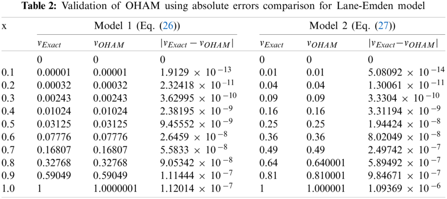
Validation of the OHAM technique is an essential part of a theoretical study. The aim of validation is to ensure the computations are reliable. For this purpose, we considered singular initial value Lane-Emden [30] model to evaluate our semi-empirical technique. Indeed, OHAM is known for its easy implementation, effectiveness for solving singular phenomena, and producing efficient results with minimum computations. The general representation of Lane-Emden equation is given as follows:
with initial conditions
where f(v) is a real valued continuous function, γ, δ and n are constants. The most common form of f(v) = vλ, here λ is tropic index. From literature it observed that the solutions of the Lane-Emden equation could be given in closed form if tropic index is 0≤ λ ≤ 5. For λ = 3, n = 2 and g(x) = x5 + 30, Eq. (25) will become:
with boundary conditions v(0) = 0 and v′(0) = 0. The exact solution of the Eq. (26) is v(x) = x5 [31].
For λ = 1, n = 2 and g(x) = x6 + 6, Eq. (25) will become:
having boundary conditions v(0) = 0 and v′(0) = 0. The exact solution of the Eq. (27) is v(x) = x2 [31].
By applying OHAM scheme Eqs. (12)–(24) subject to the given boundary conditions to evaluate solutions denoted by vOHAM. As shown in Table 2, the effectiveness of OHAM is validated using absolute errors |vExact − vOHAM|, for Eqs. (26) and (27). Table 2 verifies that accuracy is achieved even with the second order approximations.
In this section, OHAM is applied to nonlinear ODE's Eqs. (6)–(8). The homotopy of Eq. (6) is constructed as:
We consider g(η) as follows:
By solving Eqs. (28) and (29), after simplification and equating like powers of q-terms, we get
The homotopy of Eq. (7) is constructed as:
We consider ϕ(η) as follows:
By solving Eqs. (33) and (34), after simplification and equating like powers of q-terms, we get
The homotopy of Eq. (8) is constructed as:
We consider θ(η) as follows:
By solving Eqs. (37) and (38), after simplification and equating like powers of q-terms, we get
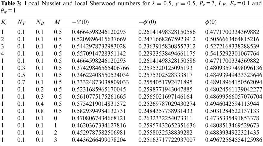
The modified equations obtained from OHAM have been solved using boundary conditions which are provided in Section 2. For solar application analysis of OHAM, solar radiation's impact in a magnetic field conducted over an extended plate with a nanofluid limit layer has been investigated to illustrate the impact of radiation parameter Velocity profile g(η) with the magnetic parameter M and γ which is ratio between μ∞(x) and μw(x). Influence on local Nusselt number ϕ′(η) and temperature profile ϕ(η) are also analyzed by varying Eckert Number Ec, magnetic field parameter M, radiation parameter Kr, Brownian motion parameter NB, Biot number λ, Prandtl number PR, thermophoresis parameter NT, and Lewis number LE. Quantitative illustration of the results for local Nusselt number and local Sherwood number for different physical quantities is provided, in Table 3. The Sherwood number θ′(η) and nanoparticle concentration Profile θ(η) are also analyzed graphically as presented below.
Velocity profile has been presented in Fig. 3 in accordance with diverse values of the magnetic parameter M with γ which is ratio between μ∞(x) and μw(x). The magnetic parameter M causes the velocity profile to decrease. Fig. 4 illustrates the diverse values of γ with fixed value of the magnetic parameter on velocity profile. It is observed with the increase in value of γ, g′(η) increases.

Figure 3: Velocity profile g′(η) for different choices of M at γ = 0.5

Figure 4: Velocity profile g′(η) for different choices of γ at M = 1
The impact of radiation parameter Kr is depicted in Fig. 5. Kr impact on temperature profile ϕ(η) is studied in detail. It is observed that increase in Kr, first increases the temperature profile ϕ(η), followed by a decrease, and lastly, an increase is illustrated. Fig. 6 shows the Nusselt Number ϕ′(η) for diverse variations of radiation parameter Kr. It is observed that increase in Kr, first decreases the ϕ′(η), followed by an increase, and lastly, a decrease is noted. Illustration of the influence of Prandtl number PR onto the dependent variable temperature profile ϕ(η) is presented in Fig. 7. Decreasing trend is observed in ϕ(η) with the increase in PR. Effect of Prandtl Number PR is studied on Nusselt number ϕ′(η) in Fig. 8. Increment in the PR makes ϕ′(η) to increase and decrement of PR causes ϕ′(η) to decrease. Hence, an increasing trend is comprehended by ϕ′(η).

Figure 5: Temperature profile ϕ(η) for different choices of radiation parameter Kr at M = 1, γ = 0.5, λ = 0.4, PR = 3, NB = 0.1, NT = 0.1, LE = 2, Ec = 0.2, ϕw = 1 showing their exciting nature

Figure 6: Nusselt number − ϕ′(η) for different choices of radiation parameter Kr at M = 1, γ = 0.5, λ = 0.4, PR = 3, NB = 0.1, NT = 0.1, LE = 2, Ec = 0.2, ϕw = 1 showing their exciting nature

Figure 7: Temperature profile ϕ(η) for different choices of Prandtl number PR at M = 0.5, γ = 0.5, λ = 0.5, Kr = 2, NB = 0.1, NT = 0.1, LE = 1, Ec = 0.2, ϕw = 1 showing their exciting nature

Figure 8: Nusselt number − ϕ′(η) for different choices of Prandtl number PR at M = 0.5, γ = 0.5, λ = 0.5, Kr = 2, NB = 0.1, NT = 0.1, LE = 1, Ec = 0.2, ϕw = 1 showing their exciting nature
Influence on temperature profile ϕ(η) in accordance with Thermophoresis parameter NT is discussed in Fig 9. The behavioral pattern comprehends it as an increasing trend. Fig. 10 shows the variation of NT on the local nusselt number ϕ′(η). This figure elucidates ϕ′(η) with a decreasing trend in accordance with the variation of NT. Brownian motion parameter NB influences on temperature profile ϕ(η) is shown in Fig. 11. The Brownian motion in nanofluids exists due to their size and because of this size the effect of its minisicule particles play an important role in transfer of heat. The basis of definition of Brownian motion; hint towards the kinetic energy of nanoparticles increasing the values of ϕ(η) due to the chaotic motion intensity. Hence, an increasing trend is comprehended in ϕ(η). Brownian motion parameter NB and its association with local Nusselt number is illustrated in Fig. 12. A decreasing trend has been comprehended by ϕ′(η) with the increase of NT.

Figure 9: Influence of NT on ϕ(η) at M = 0.5, γ = 0.5, λ = 0.5, PR = 4, Kr = 2, NB = 0.1, LE = 1, Ec = 0.2, ϕw = 1

Figure 10: Variation of NT on − ϕ′(η) at M = 0.5, γ = 0.5, λ = 0.5, PR = 4, Kr = 2, NB = 0.1, LE = 1, Ec = 0.2, ϕw = 1

Figure 11: Influence of NB on ϕ(η) at M = 0.5, γ = 0.5, λ = 0.5, PR = 4, Kr = 2, NT = 0.1, LE = 1, Ec = 0.2, ϕw = 1

Figure 12: Variation of NB on − ϕ′(η) at M = 0.5, γ = 0.5, λ = 0.5, PR = 4, Kr = 2, NT = 0.1, LE = 1, Ec = 0.2, ϕw = 1
Magnetic parameter's M effect on the temperature profile ϕ(η) is directed in Fig. 13. It is clearly noted that an increasing trend is comprehended by the ϕ(η) with the increment of M. Local Nusselt number ϕ′(η) and its resultant behavior associated with the effect of magnetic parameter M is depicted in Fig. 14. Magnetic parameter M causes a decreasing trend in ϕ′(η). Temperature profile ϕ(η) association with different values of of Lewis number LE are depicted in Fig. 15. The behavioral pattern observed from the temperature profile ϕ(η) indicates it to be that of an increasing trend. Local Nusselts Number ϕ′(η) association with the diverse values of Lewis number LE are represented in Fig. 16. The effect of LE triggers the decreasing trend in ϕ′(η) is depicted.

Figure 13: Temperature profile ϕ(η) for different choices of magnetic parameter M at Kr = 3, γ = 0.5, λ = 0.4, PR = 3, NB = 0.1, NT = 0.1, LE = 2, Ec = 0.2, ϕw = 1 showing their exciting nature

Figure 14: Nusselt number − ϕ′(η) for different choices of magnetic parameter M at Kr = 3, γ = 0.5, λ = 0.4, PR = 3, NB = 0.1, NT = 0.1, LE = 2, Ec = 0.2, ϕw = 1 showing their exciting nature

Figure 15: Temperature profile ϕ(η) for different choices of Lewis number LE at Kr = 3, γ = 0.5, λ = 0.4, PR = 3, NB = 0.1, NT = 0.1, M = 1, Ec = 0.2, ϕw = 1 showing their exciting nature

Figure 16: Nusselt number − ϕ′(η) for different choices of Lewis number LE at Kr = 3, γ = 0.5, λ = 0.4, PR = 3, NB = 0.1, NT = 0.1, M = 1, Ec = 0.2, ϕw = 1 showing their exciting nature
Temperature profile and its association with different values of Eckert Number Ec are represented in Fig. 17. The different values of Ec invoke an increasing trend in the temperature profile ϕ(η). Fig. 18 showcases the effect of Eckert Number Ec on local Nusselt numbers ϕ′(η). The increase in Ec causes an inverse influence in ϕ′(η). This means that an increase in Ec will cause a decrease in ϕ′(η). Hence, a decreasing trend is comprehended in ϕ′(η). The impact of Biot number λ is reviewed in Fig. 19 in accordance with temperature profile ϕ(η). It is observed that increase in the λ will cause an increase in the ϕ(η). Hence an increasing trend has been comprehended in the temperature profile. Biot number λ and its impact on the local Nusselt number ϕ′(η) is demonstrated in Fig. 20. It is observed that λ will cause an increase in ϕ′(η). Therefore, an increasing trend is triggered in ϕ′(η).

Figure 17: Influence of Ec on ϕ(η) at M = 0.5, γ = 0.5, λ = 0.5, PR = 4, Kr = 2, NT = 0.1, LE = 1, NB = 0.1, ϕw = 1

Figure 18: Variation of Ec on − ϕ′(η) at M = 0.5, γ = 0.5, λ = 0.5, PR = 4, Kr = 2, NT = 0.1, LE = 1, NB = 0.1, ϕw = 1

Figure 19: Influence of λ on ϕ(η) at M = 0.5, γ = 0.5, Ec = 0.4, PR = 4, Kr = 2, NT = 0.1, LE = 1, NB = 0.1, ϕw = 1

Figure 20: Variation of λ on − ϕ′(η) at M = 0.5, γ = 0.5, Ec = 0.4, PR = 4, Kr = 2, NT = 0.1, LE = 1, NB = 0.1, ϕw = 1

Figure 21: Nanoparticle concentration profile θ(η) for different choices of radiation parameter Kr at M = 1, γ = 0.5, λ = 0.4, PR = 3, NB = 0.1, NT = 0.1, LE = 2, Ec = 0.2, θw = 1 showing their exciting nature
Fig. 21 represents the Nanoparticle concentration profile θ(η) and its association with diverse values of radiation parameter Kr. It is observed that the nanoparticles are elicited inversely with different variations of the radiation parameter. Thus a decreasing trend has been comprehended in θ(η). Different variations of radiation parameter Kr on Sherwood number θ′(η) is shown in Fig. 22. The increase in Kr also originates an increase in the θ′(η). Therefore an increasing trend is comprehended in θ′(η). Different values of Prandtl number PR in association with Nanoparticle concentration profile θ(η) are presented in Fig. 23. The effect of different variations of PR trigger an increasing trend in θ(η). Prandtl number PR and its different values impact on the Sherwood number θ′(η) are revealed in Fig. 24. The different values of PR inversely effect the θ′(η). Therefore a decreasing trend is observed in θ′(η).

Figure 22: Sherwood number − θ′(η) for different choices of radiation parameter Kr at M = 1, γ = 0.5, λ = 0.4, PR = 3, NB = 0.1, NT = 0.1, LE = 2, Ec = 0.2, θw = 1 showing their exciting nature

Figure 23: Nanoparticle concentration profile θ(η) for different choices of Prandtl number PR at M = 0.5, γ = 0.5, λ = 0.5, Kr = 2, NB = 0.1, NT = 0.1, LE = 1, Ec = 0.2, θw = 1 showing their exciting nature

Figure 24: Sherwood number − θ′(η) for different choices of Prandtl number PR at M = 0.5, γ = 0.5, λ = 0.5, Kr = 2, NB = 0.1, NT = 0.1, LE = 1, Ec = 0.2, θw = 1 showing their exciting nature
The thermophoresis parameter NT and its association with Nanoparticle concentration profile θ(η) is represented in Fig. 25. The increase in NT triggers an increasing trend in θ(η). Different values of thermophoresis parameter NT and their impact on Sherwood number θ′(η) is revealed in Fig. 26. The different variations in NT cause a decreasing trend in θ′(η). Brownian motion parameter NB and its influence on Nanoparticle concentration profile θ(η) is discussed in Fig. 27. The different variations of NB elicit a decreasing trend in θ(η). Brownian motion parameter NB and its diverse values effect on the Sherwood number θ′(η) are presented in Fig. 28. It is observed that these variations elicit an increasing trend in θ′(η).

Figure 25: Influence of NT on θ(η) at M = 0.5, γ = 0.5, λ = 0.5, PR = 4, Kr = 2, NB = 0.1, LE = 1, Ec = 0.2, θw = 1

Figure 26: Variation of NT on − θ′(η) at M = 0.5, γ = 0.5, λ = 0.5, PR = 4, Kr = 2, NB = 0.1, LE = 1, Ec = 0.2, θw = 1

Figure 27: Influence of NB on θ(η) at M = 0.5, γ = 0.5, λ = 0.5, PR = 4, Kr = 2, NT = 0.1, LE = 1, Ec = 0.2, θw = 1

Figure 28: Variation of NB on − θ′(η) at M = 0.5, γ = 0.5, λ = 0.5, PR = 4, Kr = 2, NT = 0.1, LE = 1, Ec = 0.2, θw = 1
Diverse values of Lewis Number LE and their impact on the Nanoparticle concentration profile θ(η) is illustrated in Fig. 29. The sudden increment in LE resulted in somewhat greater difference because of it having weaker molecular diffusivity. This indicates that LE triggers decreasing trend in θ(η). Lewis Number LE and its different variations connotation with Sherwood number θ′(η) are illustrated in Fig. 30. The variations of LE cause an increasing trend in θ′(η). The resultant values of Nanoparticle concentration profile θ(η) due to the impact of Eckert Number Ec are discussed in Fig. 31. This indicates a decreasing trend in θ(η). Eckert number Ec and its diverse value's association with the Sherwood number θ′(η) are illustrated in Fig. 32. The Ec effects the Sherwood number θ′(η) inversely. This indicates a decreasing trend in θ′(η). Biot number λ and its diverse values impact on Nanoparticle concentration profile θ(η) is presented in Fig. 33. It is observed that the Biot Number λ elicits an increasing trend in θ(η). Fig. 34 shows the variation of Biot number λ on the Sherwood number θ′(η). It is observed that the variations of λ inversely effect the θ′(η). This indicates a decreasing trend in θ′(η).

Figure 29: Nanoparticle concentration profile θ(η) for different choices of Lewis number LE at Kr = 3, γ = 0.5, λ = 0.4, PR = 3, NB = 0.1, NT = 0.1, M = 1, Ec = 0.2, θw = 1 showing their exciting nature

Figure 30: Sherwood number−θ′(η) for different choices of Lewis number LE at Kr = 3, γ = 0.5, λ = 0.4, PR = 3, NB = 0.1, NT = 0.1, M = 1, Ec = 0.2, θw = 1 showing their exciting nature

Figure 31: Influence of Ec on θ(η) at M = 0.5, γ = 0.5, λ = 0.5, PR = 4, Kr = 2, NT = 0.1, LE = 1, NB = 0.1, θw = 1

Figure 32: Variation of Ec on −θ′(η) at M = 0.5, γ = 0.5, λ = 0.5, PR = 4, Kr = 2, NT = 0.1, LE = 1, NB = 0.1, θw = 1

Figure 33: Influence of λ on θ(η) at M = 0.5, γ = 0.5, Ec = 0.4, PR = 4, Kr = 2, NT = 0.1, LE = 1, NB = 0.1, θw = 1

Figure 34: Variation of λ on −θ′(η) at M = 0.5, γ = 0.5, Ec = 0.4, PR = 4, Kr = 2, NT = 0.1, LE = 1, NB = 0.1, θw = 1
This study exploits semi-analytical technique with changing aspects of the system. The system is based on a model with 2-D nanofluid flowing over a stretching sheet. This paper investigates the impact of Velocity profile g(η), with the magnetic parameter M and
(1) It is observed velocity profile is decreasing with the Magnetic parameter M and increasing with the γ which is ratio between μ∞(x) and μw(x).
(2) Temperature profile ϕ(η) increases with Eckert number Ec, radiation parameter Kr, thermophoresis parameter NT, magnetic parameter M, Brownian motion parameter NB, Lewis number LE, and Biot number λ. Temperature profile decreases ϕ(η) with Prandtl number PR.
(3) The increase in local Nusselt number ϕ′(η) is invoked only with Biot number λ and Prandtl number PR. The decrease in local Nusselt number ϕ′(η) is invoked with magnetic parameter M, radiation parameter Kr, Lewis number LE, Brownian motion parameter NB, thermophoresis parameter NT, and Eckert number Ec.
(4) Nanoparticle concentration profile θ(η) increased with Biot number λ, thermophoresis parameter NT and Prandtl number PR. Decreasing trend for Nanoparticle concentration profile θ(η) was observed with Brownian motion parameter NB, Lewis number LE, and Eckert number Ec and radiation parameter Kr.
(5) Trend for Sherwood number θ′(η) was observed to increase with radiation parameter Kr, Lewis number LE, and Brownian motion parameter NB. Trend for Sherwood number θ′(η) was observed to decrease with Eckert number Ec, thermophoresis parameter NT, Biot number λ and Prandtl number PR.
Funding Statement: The authors received no specific funding for this study.
Conflicts of Interest: The authors declare that they have no conflicts of interest to report regarding the present study.
1. Hua, X., Zeng, Y., Wang, W., Shen, W. (2014). Light absorption mechanism of c-Si/a-Si half-coaxial nanowire arrays for nanostructured heterojunction photovoltaics. IEEE Transactions on Electron Devices, 61(12), 4007–4013. DOI 10.1109/TED.2014.2363001. [Google Scholar] [CrossRef]
2. de Wild, J., Duindam, T., Rath, J., Meijerink, A., van Sark, W. et al. (2012). Increased upconversion response in a-Si: H solar cells with broad-band light. IEEE Journal of Photovoltaics, 3(1), 17–21. DOI 10.1109/JPHOTOV.2012.2213799. [Google Scholar] [CrossRef]
3. Pakhuruddin, M. Z., Huang, J., Dore, J., Varlamov, S. (2015). Light absorption enhancement in laser-crystallized silicon thin films on textured glass. IEEE Journal of Photovoltaics, 6(1), 159–165. DOI 10.1109/JPHOTOV.5503869. [Google Scholar] [CrossRef]
4. Chen, M., Zhang, Y., Cui, Y., Zhang, F., Qin, W. et al. (2017). Profiling light absorption enhancement in two-dimensional photonic-structured perovskite solar cells. IEEE Journal of Photovoltaics, 7(5), 1324–1328. DOI 10.1109/JPHOTOV.2017.2719759. [Google Scholar] [CrossRef]
5. Ishizaki, K., Motohira, A., De Zoysa, M., Tanaka, Y., Umeda, T. et al. (2017). Microcrystalline-silicon solar cells with photonic crystals on the top surface. IEEE Journal of Photovoltaics, 7(4), 950–956. DOI 10.1109/JPHOTOV.2017.2695524. [Google Scholar] [CrossRef]
6. Mehmood, U., Al-Ahmed, A., Afzaal, M., Hakeem, A. S., Haladu, S. A. et al. (2018). Enhancement of the photovoltaic performance of dye-sensitized solar cells by cosensitizing TiO2 photoanode with uncapped pbs nanocrystals and ruthenizer. IEEE Journal of Photovoltaics, 8(2), 512–516. DOI 10.1109/JPHOTOV.5503869. [Google Scholar] [CrossRef]
7. Liang, H., Liu, Y., Li, H., Zhang, H., Han, S. et al. (2018). All-fiber light intensity detector based on an ionic-liquid-adorned microstructured optical fiber. IEEE Photonics Journal, 10(2), 1–8. DOI 10.1109/JPHOT.4563994. [Google Scholar] [CrossRef]
8. Ishii, S., Sugavaneshwar, R. P., Nagao, T. (2016). Titanium nitride nanoparticles as plasmonic solar heat transducers. The Journal of Physical Chemistry C, 120(4), 2343–2348. DOI 10.1021/acs.jpcc.5b09604. [Google Scholar] [CrossRef]
9. Gondal, M., Rashid, S., Dastageer, M., Zubair, S., Ali, M. et al. (2013). Sol-gel synthesis of {Au/Cu−TiO2} nanocomposite and their morphological and optical properties. IEEE Photonics Journal, 5(3), 2201908–2201908. DOI 10.1109/JPHOT.2013.2262674. [Google Scholar] [CrossRef]
10. Hogan, N. J., Urban, A. S., Ayala-Orozco, C., Pimpinelli, A., Nordlander, P. et al. (2014). Nanoparticles heat through light localization. Nano Letters, 14(8), 4640–4645. DOI 10.1021/nl5016975. [Google Scholar] [CrossRef]
11. Ishii, S., Sugavaneshwar, R. P., Chen, K., Dao, T. D., Nagao, T. (2016). Solar water heating and vaporization with silicon nanoparticles at mie resonances. Optical Materials Express, 6(2), 640–648. DOI 10.1364/OME.6.000640. [Google Scholar] [CrossRef]
12. Wang, Z., Tao, P., Liu, Y., Xu, H., Ye, Q. et al. (2014). Rapid charging of thermal energy storage materials through plasmonic heating. Scientific Reports, 4(1), 1–8. DOI 10.1038/srep06246. [Google Scholar] [CrossRef]
13. Ghasemi, S. E., Hatami, M., Sarokolaie, A. K., Ganji, D. (2015). Study on blood flow containing nanoparticles through porous arteries in presence of magnetic field using analytical methods. Physica E: Low-Dimensional Systems and Nanostructures, 70, 146–156. DOI 10.1016/j.physe.2015.03.002. [Google Scholar] [CrossRef]
14. Ghasemi, S. E., Hatami, M., Hatami, J., Sahebi, S., Ganji, D. (2016). An efficient approach to study the pulsatile blood flow in femoral and coronary arteries by differential quadrature method. Physica A: Statistical Mechanics and its Applications, 443, 406–414. DOI 10.1016/j.physa.2015.09.039. [Google Scholar] [CrossRef]
15. Valipour, P., Ghasemi, S., Vatani, M. (2015). Theoretical investigation of micropolar fluid flow between two porous disks. Journal of Central South University, 22(7), 2825–2832. DOI 10.1007/s11771-015-2814-1. [Google Scholar] [CrossRef]
16. Vatani, M., Ghasemi, S., Ganji, D. (2016). Investigation of micropolar fluid flow between a porous disk and a nonporous disk using efficient computational technique. Proceedings of the Institution of Mechanical Engineers, Part E: Journal of Process Mechanical Engineering, 230(6), 413–424. DOI 10.1177/0954408914557375. [Google Scholar] [CrossRef]
17. Ghasemi, S., Hatami, M., Ganji, D. (2013). Analytical thermal analysis of air-heating solar collectors. Journal of Mechanical Science and Technology, 27(11), 3525–3530. DOI 10.1007/s12206-013-0878-0. [Google Scholar] [CrossRef]
18. Ghasemi, S. E. (2017). Thermophoresis and brownian motion effects on peristaltic nanofluid flow for drug delivery applications. Journal of Molecular Liquids, 238, 115–121. DOI 10.1016/j.molliq.2017.04.067. [Google Scholar] [CrossRef]
19. Ibrahim, W., Shankar, B., Nandeppanavar, M. M. (2013). Mhd stagnation point flow and heat transfer due to nanofluid towards a stretching sheet. International Journal of Heat and Mass Transfer, 56(1), 1–9. DOI 10.1016/j.ijheatmasstransfer.2012.08.034. [Google Scholar] [CrossRef]
20. Mushtaq, A., Mustafa, M., Hayat, T., Alsaedi, A. (2014). Nonlinear radiative heat transfer in the flow of nanofluid due to solar energy: A numerical study. Journal of the Taiwan Institute of Chemical Engineers, 45(4), 1176–1183. DOI 10.1016/j.jtice.2013.11.008. [Google Scholar] [CrossRef]
21. Ghasemi, S. E., Hatami, M., Jing, D., Ganji, D. (2016). Nanoparticles effects on mhd fluid flow over a stretching sheet with solar radiation: A numerical study. Journal of Molecular Liquids, 219, 890–896. DOI 10.1016/j.molliq.2016.03.065. [Google Scholar] [CrossRef]
22. Mushtaq, A., Mustafa, M., Hayat, T., Alsaedi, A. (2014). Nonlinear radiative heat transfer in the flow of nanofluid due to solar energy: A numerical study. Journal of the Taiwan Institute of Chemical Engineers, 45(4), 1176–1183. DOI 10.1016/j.jtice.2013.11.008. [Google Scholar] [CrossRef]
23. Awan, S. E., Raja, M. A. Z., Mehmood, A., Niazi, S. A., Siddiqa, S. (2020). Numerical treatments to analyze the nonlinear radiative heat transfer in mhd nanofluid flow with solar energy. Arabian Journal for Science and Engineering, 45, 4975–4994. DOI 10.1007/s13369-020-04593-5. [Google Scholar] [CrossRef]
24. Marinca, V., Herisanu, N. (2015). Optimal homotopy asymptotic method. In: The optimal homotopy asymptotic method, pp. 9–22. Germany: Springer. [Google Scholar]
25. Marinca, V., Herisanu, N. (2008). Application of optimal homotopy asymptotic method for solving nonlinear equations arising in heat transfer. International Communications in Heat and Mass Transfer, 35(6), 710–715. DOI 10.1016/j.icheatmasstransfer.2008.02.010. [Google Scholar] [CrossRef]
26. Herisanu, N. (2020). Optimal homotopy asymptotic approaches to nonlinear dynamical systems in engineering-4. AIP Conference Proceedings, vol. 2293. AIP Publishing LLC. [Google Scholar]
27. Marinca, V., Herisanu, N. (2010). Optimal homotopy perturbation method for strongly nonlinear differential equations. Nonlinear Science Letters A, 1(3), 273–280. [Google Scholar]
28. Iqbal, S., Javed, A. (2011). Application of optimal homotopy asymptotic method for the analytic solution of singular lane-emden type equation. Applied Mathematics and Computation, 217(19), 7753–7761. DOI 10.1016/j.amc.2011.02.083. [Google Scholar] [CrossRef]
29. Manzoor, T., Nazar, K., Iqbal, S., Manzoor, H. U. (2021). Theoretical investigation of unsteady mhd flow within non-stationary porous plates. Heliyon, 7(3), e06567. DOI 10.1016/j.heliyon.2021.e06567. [Google Scholar] [CrossRef]
30. Lane, H. J. (1870). On the theoretical temperature of the sun, under the hypothesis of a gaseous mass maintaining its volume by its internal heat, and depending on the laws of gases as known to terrestrial experiment. American Journal of Science, 2(148), 57–74. DOI 10.2475/ajs.s2-50.148.57. [Google Scholar] [CrossRef]
31. Wazwaz, A. M. (2001). A new algorithm for solving differential equations of lane-emden type. Applied Mathematics and Computation, 118(2), 287–310. DOI 10.1016/S0096-3003(99)00223-4. [Google Scholar] [CrossRef]
 | This work is licensed under a Creative Commons Attribution 4.0 International License, which permits unrestricted use, distribution, and reproduction in any medium, provided the original work is properly cited. |