Computer Modeling in Engineering & Sciences

DOI: 10.32604/cmes.2022.017663

ARTICLE

Time Synchronized Velocity Error for Trajectory Compression

Haibao Jiang1, Dezhi Han1,*, Han Liu1, Jiuzhang Han1 and Wenjing Nie2

1College of Information Engineering, Shanghai Maritime University, Shanghai, 201306, China
2College of Foreign Language, Shanghai Maritime University, Shanghai, 201306, China
*Corresponding Author: Dezhi Han. Email: dezhihan88@sina.com
Received: 28 May 2021; Accepted: 20 August 2021

1  Introduction

Positioning technology is developing rapidly while the equipment is in and portable. The equipment obtains a large scale of trajectory data on various moving objects such as vehicles, humanities, animals, etc. That information, affluent and worthy, is contained in trajectory data and has applied widely to the fields such as behavioral analysis [1–3], regional analysis [4,5], and urban functions and computing [6–9]. The huge amount of data usually contains much redundant information, which brings enormous challenges to data storage, query and analysis, as well as transmission. To solve the above-mentioned problems, researchers have proposed outstanding and numerous algorithms of trajectory compression in the past decades [10–30]. These algorithms acquire the time and the rate of compression by losing the accuracy within the allowable error range and thus to meet the requirements in special situations.

When we compress the trajectory, the methods usually use distance to evaluate the error. Douglas et al. [11,13] used the Perpendicular Euclidean Distance (PED) as the criterion of the split points in compression, then it became one of the most common methods to evaluate the error of the compression. This method can accurately describe the geometric error between the compressed and the raw trajectory. Meratnia et al. [14] provided a mathematical model, Time-Ratio Distance metric (TRD), by calculating the distance between the raw and the projected position, which was calculated by the temporal scale of the compressed trajectory, as the error. Potamias et al. [17] proposed to use Time Synchronized Euclidean Distance (SED) as the criterion of error aim at maintaining the time information on the compressed trajectory. While predicts the position it differs from TRD by considering the velocity vector, rather than just the temporal scale. They both assumed that the object moved uniformly in the compressed trajectory, so the results are similar. Liu et al. [18] proposed a continuous method, namely Enclosed Area (EA), which calculated the area between the raw and the compressed trajectory segment as the error and was more accurate than predecessors’ method which was discrete, but for its low calculation efficiency it was seldom applied.

However, the velocity is ignored in the above-mentioned methods. In fact, the velocity is the foremost in trajectory compression as it contains more valuable information. Trajectory points with similar velocities usually represent the same type of motion along the direction, while the points with obvious velocity variation may imply changes in motion conditions [19]. Changes in geometric structure are usually reflected in velocity, but changes in velocity may not be showed in the structure. For example, a shift in means of transport is often embodied in the velocity but not the structure. Therefore, it is of great significance to evaluate the velocity error.

To fill the above gap, this paper proposes a mathematical model for evaluating velocity error in the trajectory compression, Time Synchronized Velocity Error (SVE). The main difference between the SVE and the state-of-the-art methods is the constraints of compression, as the former uses time synchronization velocity instead of distance that can improve quality. The model, found on the hypothesis of linear velocity variation (see Section 2.2 of this paper for details) can evaluate the error effectively, conveniently and accurately. On this basis, we come up with an innovative algorithm of trajectory compression, i.e., Minimum Time Synchronized Velocity Error Based on Sliding Window (SW-MSVE). Based on the Sliding Window, this algorithm preserves the minimum velocity error in the compression with low time complexity. The reliability of the SVE model and the SW-MSVE algorithm is experimentally verified in the Geolife [31–33].

The main contributions in this paper can be summarized as follows:

(1) We propose the new concept of time synchronized velocity. Based on the assumption of velocity changes linearly, the velocity of the compressed point in both latitude and longitude directions can be accurately calculated, which in turn can be used to evaluate the velocity errors generated during the trajectory compression.

(2) A novel mathematical model for evaluating compression error is designed, namely SVE. This model uses the time synchronized velocity as constraint instead of distance which can evaluate the compression error more effectively, conveniently, and accurately.

(3) An innovative algorithm of the trajectory compression is proposed, namely SW-MSVE, which can minimize the velocity error under the premise at local optimization. This algorithm preserves more information of the raw trajectory in the compression with the low time complexity and can be applied to both offline and online.

(4) Two elaborate experiments are designed to demonstrate the advancements of the SVE and the SW-MSVE respectively. In the first experiment, we use the PED, the SED and the SVE to evaluate the error under four compression algorithms, one of which is the SW-MSVE algorithm. The results show that the SVE is less influenced by noise with stronger performance and more applicability. In the second experiment, we compare the SW-MSVE algorithm with three others algorithms at information retention. The results show that the SW-MSVE algorithm can take into account both velocity and geometric structure constraints and retains more information of the raw trajectory at the same compression ratio.

The remainder of the article is organized as follows. A background of the theories will be presented scientifically in Section 2. The process of building the SVE mathematical model and the working principle of the SW-MSVE algorithm will be introduced in Section 3. Section 4 contains the fully experimental procedures and processing operations, followed by the discussion of test results in Section 5. Finally, conclusions will be offered in Section 6.

2  Background

This chapter systematically introduces the theories used in this paper. We introduce the concept of trajectory compression firstly. Secondly, we illustrate the principle of three classical compression algorithms with examples. The algorithms are Douglas-Peucker (DP) [11], Top-Down Time-Ratio (TD-TR) [12], and Sliding Window (SW) [14] respectively. Finally, we introduce the computing methods of PED and SED.

2.1 Concepts and Methods of Trajectory Compression

In the allowable error range, trajectory compression is eliminating the raw trajectory point which take along the redundant information. Then we can obtain a compressed trajectory with smaller scale, lower redundancy which is similar to the raw one. Fig. 1 illustrates the concept of trajectory compression. The raw trajectory is shown in Fig. 1a and has 12 points. As shown in Fig. 1b, they are compressed to 4 points, which are the starting point P1, the intermediate points P4 and P8, and the ending point P12 (the starting point and the ending point should be retained in the trajectory compression). The compressed trajectory only occupies one third of the space in the raw trajectory but basically retains the information of original movement.

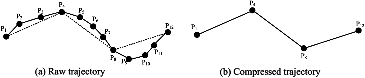
Figure 1: Trajectory compression concept (a) Raw trajectory (b) Compressed trajectory

Researchers have proposed outstanding and numerous methods stand on the requirements of the trajectory compression. These methods are technically divided into three categories, line simplification compression methods [11–22], Map-matching based compression methods [23–27], and semantic compression methods [28–30]. The methods used in this paper belong to the first category and their working principles are separately described as below.

The Douglas-Peucker (DP) algorithm can preserve the spatial geometry of the raw trajectory in the compression and the key is to use several baselines and replace the trajectory. Firstly, the starting and ending points of the trajectory are connected as an approximate segment. Secondly, the PED is calculated for the intermediate points in turn (see Section 2.2 of this paper for details) and the algorithm selects the point that has the largest PED. If the PED of this point is above the specified threshold of the algorithm, then it will be added to the compressed trajectory and be selected as the split point which divides the trajectory into two sub-trajectories. the above operations should be repeated until all the points are unavailable to be the split point. The steps will be illustrated in Example 1 below:

Example 1: The trajectory T contains {P1,P2,P3,P4,P5,P6,P7,P8,P9,P10,P11,P12} 12 points, in which P1 is the starting point while P12 is the ending point. According to the principle of the DP algorithm, as shown in Fig. 2a, the first step is to connect P1 and P12 as a baseline and calculate the PED of the remaining points, respectively. We find the point P9 with the maximum PED, i.e., dmax. Obviously, the PED of P9 is above the threshold, i.e., dmax>d, the point is selected as the split point (reserved point) so the T is divided into T1{P1,P2,P3,P4,P5,P6,P7,P8,P9} and T2{P9,P10,P11,P12}. In the second step, as shown in Fig. 2b, we find the point P4 in T1 with the maximum PED and dmax>d, so the next step continues to compress T1 with P4 as the second split point. The PED of all points in T2 is smaller than the threshold, thus the points P10 and P11 will be compressed and then the compression of the T2 part is finished.

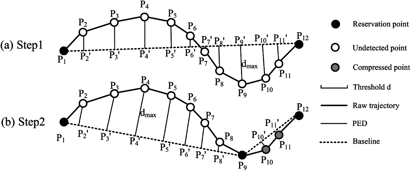
Figure 2: DP algorithm (a) Step 1 (b) Step 2

The DP algorithm has widely is applied in various fields for its simple ideas and better performance in both compression ratio and accuracy However, it has two disadvantages. Firstly, the time complexity of the algorithm is as high as O(nlogn). Secondly, the algorithm just considers the spatial factor without the time and velocity factor in the compression, so the compressed trajectory only resembles the raw trajectory in geometry.

Based on the idea of the DP, the Top-Down Time-Ratio (TD-TR) algorithm uses a new distance function, namely SED (see Section 2.2 of this paper for details). Firstly, it finds the corresponding position of the original points on the baseline according to the velocity proportion and then calculates the Euclidean distance between the compressed and the original point. During this process, it selects the point that has the largest SED. If the SED of the point is greater than the specified threshold of the algorithm, then it will be added to the compressed trajectory and is selected as the split point which divides the trajectory into two sub-trajectories. the above operations should be repeated until all the points are unavailable to be the split point. The steps will be illustrated in Example 2 below:

Example 2: As shown in Fig. 3, the trajectory T contains {P1,P2,P3,P4,P5,P6,P7,P8,P9,P10,P11,P12} 12 points, in which P1 is the starting point while P12 is the ending point. According to the principle of TD-TR algorithm, as shown in Fig. 3a, the first step is to connect P1 and P12 as a baseline and calculates the SED of the remaining points, respectively. We find the point P4 with the maximum SED, i.e., dmax. Obviously, the SED of P4 is above the threshold, i.e., dmax>d, the point is selected as the split point (reserved point) so the T is divided into T1{P1,P2,P3,P4} and T2{P4,P5,P6,P7,P8,P9,P10,P11,P12}. In the second step, as shown in Fig. 3b, the SED of all points in T1 is smaller than the threshold, so the compression of T1 part is finished. We find the point P9 in T2 with the maximum SED and dmax>d, so the next step continues to compress T2 with P9 as the second split point.

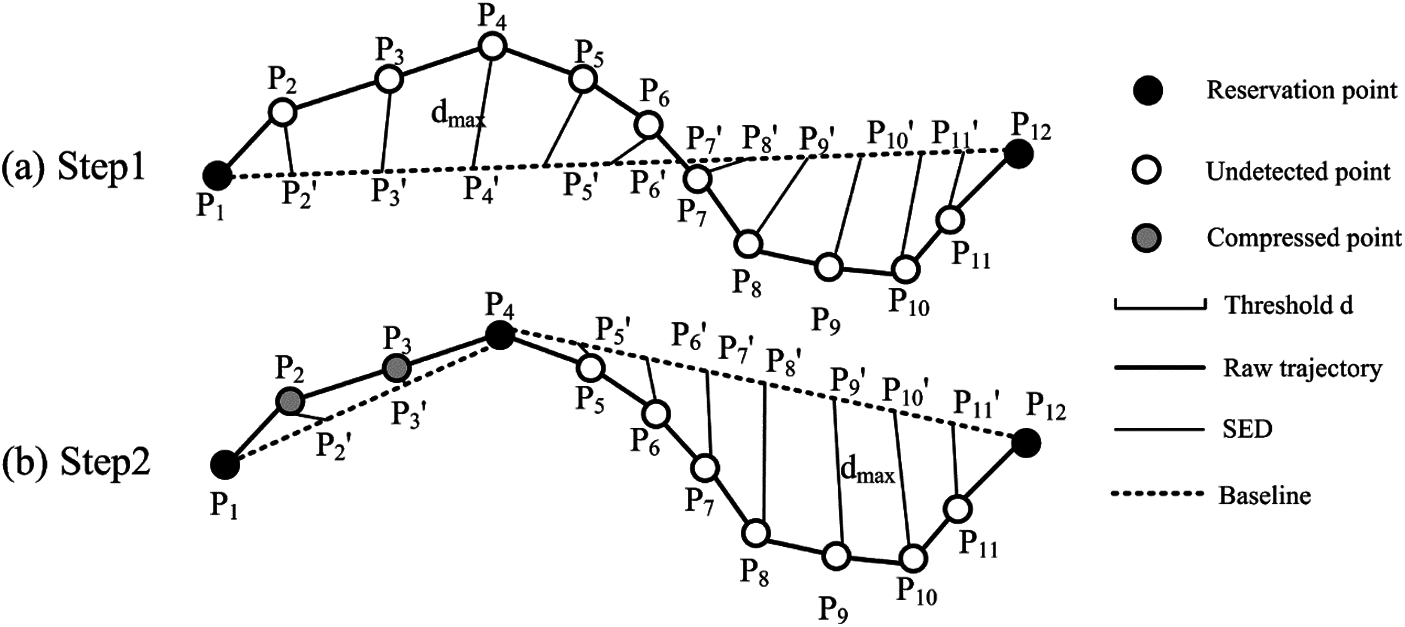
Figure 3: TD-TR algorithm (a) Step 1 (b) Step 2

The TD-TR algorithm has all the advantages of the DP and more accurate error because the SED considers both time and spatial factors. But it still has disadvantages including the following two points. Firstly, the time complexity of the algorithm is O(nlogn). Secondly, the velocity factor of the points is not sufficiently considered in the compression.

The Sliding Window (SW) algorithm is one of the online compression techniques, which can compress trajectories with the premise at local optimum. The elemental idea is to eliminate the noise point by a window. The first step is to connect the starting point and the ending point in the window as the approximate segment and calculate the PED between the intermediate point and the segment. If it is smaller than the specified threshold of the algorithm, the window moves forward one bit and adds a new intermediate point. Otherwise, the intermediate point is used as a new starting point of the window and the calculation continues until the window moves to the last bit. The steps will be illustrated in Example 3 below:

Example 3: The trajectory T contains {P1,P2,P3,P4,P5,P6} 6 trajectory points, in which P1 is the starting point while P6 is the ending point. According to the principle of the SW algorithm, as shown in Fig. 4a, the first step is to connect P1 and P3 as a baseline and calculates the PED between P2 and the baseline. Obviously, d2<d, P2 can be compressed and the window moves forward one bit. The second step is as shown in Fig. 4b. Similarly, d3>d, P3 is set as the reserved point and become the starting point of the window, then it moves forward one bit. The case of the third and fourth steps is the same as the first step. When the sliding window moves to P6, it means the algorithm is executed to the last step.

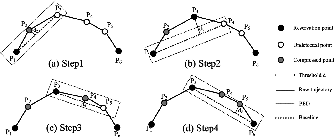
Figure 4: SW algorithm (a) Step 1 (b) Step 2 (c) Step 3 (d) Step 4

The SW algorithm has high execution efficiency with time complexity only O(n) and can compress the raw trajectory at local optimum, which ensures the compression ratio and accuracy. But it still cannot avoid the following two main disadvantages. Firstly, it cannot achieve the global optimum. Secondly, it only considers the space factor but ignores the time and velocity factor.

2.2 Error Evaluation Methods for Trajectory Compression: PED and SED

The PED is the point-to-line distance from the trajectory point to the baseline, while the SED is essentially the point-to-point distance. The PED and the SED represent the distance from Pi to Pi′ in Figs. 5a and 5b, respectively. In Fig. 5a, the PED of point P2 is the distance from P2 to the baseline P1P7. In Fig. 5b, assuming that the object moves uniformly in baseline P1P7, The points (P2′,P3′,P4′,P5′,P6′) are added equidistantly on P1P7 and the SED of point P2 represents the distance from point P2 to P2′.

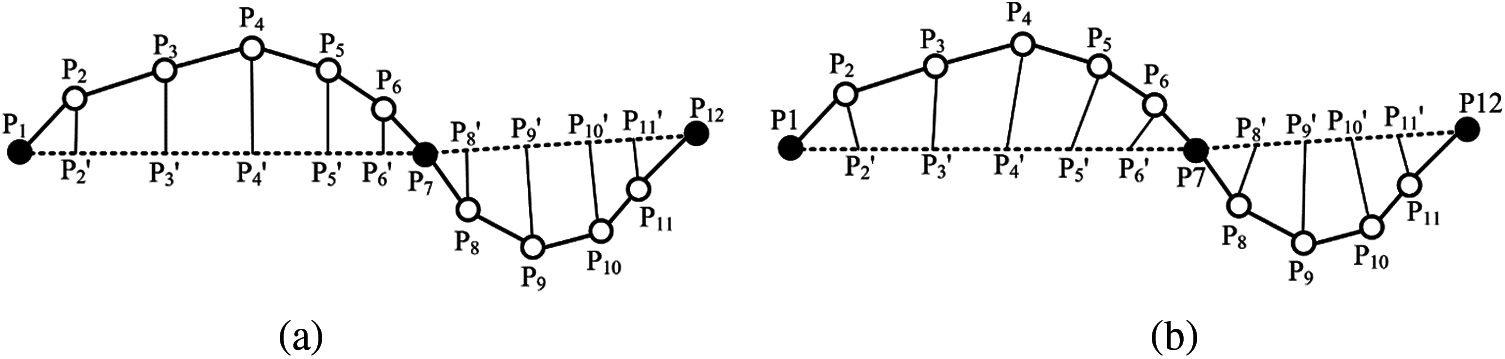
Figure 5: Trajectory compression error evaluation methods: (a) PED; (b) SED

These methods provide an accurate measure of the error in the distance between the compressed and the raw trajectory. During the trajectory compression, the PED or the SED value is larger, the compressed trajectory is less geometrically similar to the raw one. On the contrary, the compressed trajectory is similar to the raw trajectory while the value of the PED or the SED is smaller.

3  SVE Mathematical Model and SW-MSVE Algorithm

We build a mathematical model to describe the velocity error during the trajectory compression and two assumptions are proposed for the trajectory sequence:

A1: The velocities of the moving object are both 0 m/s in the directions of longitude and latitude at the start and end positions.

A2: The velocity of the moving object varies linearly between two adjacent points of the trajectory, such as uniform acceleration, uniform velocity, uniform deceleration, etc.

3.1 Time Synchronization Velocity

Based on the assumption A2, we propose a new concept to quantify the velocity during the trajectory compression, i.e., the Time Synchronization Velocity. The calculation principle is shown in Fig. 6 and the formula is shown in formula (1):

vm′=vS+tm−tste−ts(ve−vs), (1)

where s, m and e denote the serial number of starting point, intermediate point and ending point of the sub-trajectory segment, respectively. vm′ denotes the calculated time synchronization velocity, vS and ve denote the velocity of starting point and the ending point of the sub-trajectory segment, respectively, ts,tm,te denote the time of starting point, intermediate point and ending point of the sub-trajectory segment, respectively.

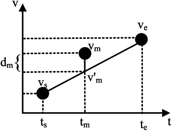
Figure 6: Schematic diagram of the time synchronization velocity error calculation method

3.2 Velocity of Trajectory Points

According to the raw trajectory, we calculate the distance between the adjacent points in the directions of longitude and latitude firstly. Since the earth is an ellipsoid, the distance cannot be obtained only by subtracting the position and the actual situation must be fully considered. We should hold the following formula while calculating the velocity of a point in the directions of longitude and latitude:

Ldi+1=Lpi+1−Lpi, (2)

where Ldi denote the difference in latitude or longitude of the ith and i+1th trajectory points, which can be expressed as xdi and ydi, respectively. Lpi refers to the current latitude and longitude coordinates, which can be expressed as xpi and ypi, respectively.

Xdi=xdiπ180R, (3)

r=Rcosxpi, (4)

Ydi=ydiπ180r, (5)

According to the above formulas (2)–(5), we can deduce that:

Xdi=(xpi+1−xpi)π180R, (6)

Ydi=(ypi+1−ypi)π180Rcosxpi, (7)

where Xdi,Ydi denote the actual distance in latitude and longitude of the ith and i+1th trajectory points, respectively. R denotes the distance of the current trajectory point from the earth’s center. r denotes the radius of the current latitudinal section circle, and π, the ratio of circumference to diameter.

Based on the assumption A1 and A2, we calculate the velocity of each trajectory point by formulas (6) and (7).

vxpi+i+12=Xditi+1−ti, (8)

vypi+i+12=Yditi+1−ti, (9)

vxpi+1=vxpi+2(vxpi+i+12−vxpi), (10)

vypi+1=vypi+2(vypi+i+12−vypi), (11)

where vxpi+i+12 and vypi+i+12 denote average velocity of the ith and i+1th trajectory points in the directions of longitude and latitude, respectively. vxpi and vypi denote the velocity in the directions of latitude or longitude of the ith and i+1th trajectory points, respectively. ti denotes the acquisition time of the ith trajectory point.

According to the above formulas (6), (7), (10) and (11), we can deduce that:

vxpi+1=2(xpi+1−xpi)π(ti+1−ti)180R−vxpi, (12)

vypi+1=2(ypi+1−ypi)π(ti+1−ti)180Rcosxpi−vypi. (13)

3.3 SVE Mathematical Model

Fig. 6 shows the calculative principle of the time synchronized velocity error and we can calculate the error dm as follows:

dm=|vm−vm′|, (14)

where vm denotes the velocity of the trajectory point with serial number m, dm denotes the absolute value of the difference between the actual measured and the time synchronous velocity. If the velocity varies linearly, the velocity error at this moment is 0 m/s based on the formula (14) of the time synchronous velocity.

We define the raw trajectory sequence as T, T={P1,P2,P3,…,Pn}, in which Pi denotes the ith (i=1,2,3,…,n) trajectory point of the T and each point is denoted as Pi(xpi,ypi,tpi). Define the compressed trajectory as T′, T′={P1,…,Pi,…,Pn}. Then the mathematical model of velocity error in the trajectory compression is shown as follows.

Firstly, the original latitude and longitude velocity lists are calculated from assumption A1 and formulas (12) and (13).

vxT={vxp1,vxp2,vxp3,…,vxpn}, (15)

vyT={vyp1,vyp2,vyp3,…,vypn}, (16)

where vxT denotes the raw trajectory latitude velocity sequence and vyT denotes the raw trajectory longitude velocity sequence.

Then we respectively calculate the latitude and longitude velocity list of the compressed trajectory by the time synchronized velocity formula. The transformation is that the velocities of the points in the T′ are kept as the same as the original points. The time synchronized velocity of the compressed points is calculated and added to the corresponding velocity list according to formula (1).

vxT′={vxp1,vxp2′,vxp3′,…vxps…,vxpn}, (17)

vyT′={vyp1,vyp2′,vyp3′,…vyps…,vypn}, (18)

where vxT′, vyT′ denote the velocity list of the compressed trajectory in latitude and longitude, respectively. vxpi′, vypi′ denote the time synchronized velocity of the ith trajectory point after the calculation of formula (1), respectively.

Finally, we calculate the velocity error between the raw and the compressed trajectory according to formula (14) and average the error to obtain the SVE. The method of calculation is shown in formulas (19) and (20).

vxerror=∑i=1ndxin, (19)

vyerror=∑i=1ndyin, (20)

where vxerror denotes the average SVE in the latitude direction (LAT) and vyerror denotes the average SVE in the longitude direction (LON).

The average SVE during the whole trajectory compression is:

verror=∑i=1ndxi+dyin. (21)

3.4 SVE Evaluation Process

Fig. 7 shows the flow chart of the SVE to evaluate the error of trajectory compression. Firstly, input the raw trajectory and calculate the velocities in both directions of latitude and longitude respectively. Secondly, compress the raw trajectories by various algorithms and obtain the compressed trajectories. Then, based on the assumption of the velocity varying linearly, calculate the error between the time synchronous velocity and the actual velocity of each point and get the SVE of the compressed trajectory on average.

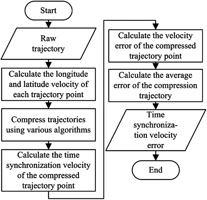
Figure 7: Flowchart of the SVE mathematical model to evaluate the trajectory compression error

3.5 SW-MSVE Algorithm

The principle of the SW-MSVE algorithm is shown in Alogrithm1. Based on the assumption of the velocity varying linearly, the SW-MSVE uses the sum of time synchronized velocity error in the directions of latitude and longitude as the distance function in the sliding window and can minimize the velocity error in the compression. However, this value is only the minimum velocity error under the premise at local optimization.

Before executing the algorithm, input the raw trajectory T and the threshold Ω, where the Ω is used to determine whether the trajectory points satisfy the compression condition by the current sliding window. Firstly, calculate the velocity list of latitude vxT and longitude vyT by formulas (12) and (13). Secondly, calculate the SVE and compare it with the threshold Ω for all intermediate points. Then move the intermediate points and ending point in the window forward one bit regardless of the result. If dxi+dyi≥ Ω, it means that the variation in velocity is large and cannot be compressed. Conversely, the point has little variation in velocity and can be compressed, whereupon the serial number of the point is added to the compressible list. Finally, delete the point in the compressible list in the raw trajectory T. Obtain the compressed trajectory T′ and output it which can end the algorithm.

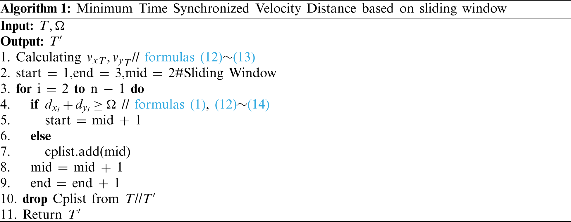
The time complexity of Step 1 in the algorithm is O(2n), Steps 2–9 are O(n), Step 10 is O(n), and Step 11 is O(1). Therefore, the total time complexity is O(n). The elements of each position are visited in the algorithm and the complexity is not greater than the time complexity O(n), so the space complexity is also O(n).

The SW-MSVE inherits all the advantages of the SW algorithm, such as low time complexity and high execution efficiency. The algorithm uses the SVE as the error and considers both time and velocity dimensions, thus it can guarantee the geometric similarity of the compressed and the raw trajectory. Another advantage of the algorithm will be verified through subsequent experiments in this paper.

4  Experiment and Results

To demonstrate the performances of the SVE and the SW-MSVE, we perform an experiment on the Geolife [31–33] dataset. We compare and analyze the variations of the PED, the SED and the SVE with compression ratio for the DP, TD-TR, SW and SW-MSVE algorithms. The experimentation is shown in Fig. 8. Firstly, input the raw trajectory data and filter out the noise points. Secondly, use four algorithms to compress the data. The experiment compares and analyzes the evaluation effects of the PED and the SVE under the DP algorithm, the SED and the SVE under TD-TR algorithm, the PED, the SED and the SVE under the SW and SW-MSVE algorithms. Finally, verify the advantage of the SW-MSVE in information retention by labeling the raw trajectory points.

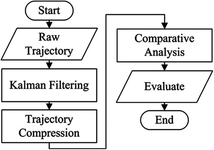
Figure 8: Experimental process

4.1 Experimental Data and Environment

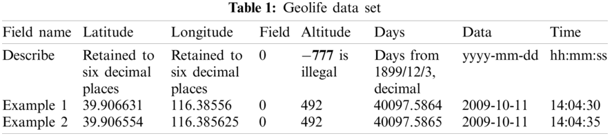
The original data of this experiment is collected from user 000 in the Geolife project (Microsoft Research Asia). The dataset includes 17,621 trajectories with a total distance of 1,292,951 km and a total duration of 50,176 h. Table 1 shows the format of the dataset. Each raw trajectory is saved in a PLT file, of which the first 6 rows are useless information that can be ignored and the data are organized starting from row 7. This experiment only extracts four attributes of data: Latitude, Longitude, Data, and Time.

The detailed experimental environment for this paper is shown below:

CPU: Intel(R) Core (TM) i5-6500 CPU@3.20 GHz, 3.192 Mhz.

RAM: 8G.

Operating system: Windows 10 Professional.

Compiler environment: Anaconda 2020.07; Jupyter notebook 6.0.3; Python 3.8.3;

Data package: Pandas, Matplotlib, Numpy, etc.

4.2 Trajectory Filtering

During the trajectory sequences collecting, there are often some disturbing factors that make a few points, which we call noise points, to appear in unreasonable positions. These points are small in scale but will affect the quality in trajectory compression. Filtering is important in those situations where the trajectory data is particularly noisy, or when one wants to derive other quantities from it, like speed or direction [34]. Therefore, the trajectory must be filtered before conducting the compression experiment. The common processing methods are Median filtering, Mean filtering, Kalman filtering, and Particle filtering. We compare the applicability of the four methods to the trajectory data and the need of the subsequent experiments, the Kalman filter was chosen to process the experimental data.

Kalman Filtering [34] is an algorithm that uses the state equation of a linear system to optimally estimate the system state from input and output observations. The specific steps and parameters are shown below:

Z^k′=AZ^k−1, (22)

Pk′=APk−1AT+Q′, (23)

Kk=Pk′HTHPk′HT+R′, (24)

Z^k=Z^k′+Kk(Zk−HZ^k′), (25)

Pk=(I−KkH)Pk′, (26)

At the kth point of the trajectory sequence, Z^k′ denotes the priori estimated position of the current trajectory point. Z^k denotes the posteriori estimated position of the current point. Zk denotes the actual measurement position of the current point. Pk′ denotes the a priori error covariance of the current point. Kk denotes the Kalman gain of the current point. Pk denotes the error covariance of the current point. A denotes the state transfer matrix. Q′ denotes the process noise. R′ denotes the measurement noise. H denotes the measurement matrix. and I denotes the unit matrix. Using the formulas (22)–(26), the trajectory sequence is filtered to avoid the interference of noisy points to the subsequent calculation. The values of each parameter are taken as shown below, where, tk denotes the kth and k-1th trajectory point time interval. xp0, yp0 denote the latitudinal and longitudinal velocity sequences at the start of the trajectory sequence, respectively. The values of P0, Q and R′ can be adjusted appropriately.

P0=[0.000100000.000100000.000900000.0009], (27)

Q′=[0.000100000.000100000.000400000.0004], (28)

A=[10000100tk0100tk01], (29)

I=[1000010000100001], (30)

R′=[0.1000.1], (31)

H=[10010000], (32)

z^0=[xp0yp000], (33)

The filter’s threshold Ω′ is set 0.001 (the threshold can be set to other values) and determines whether the error between the posteriori estimated position Z^k and the measured position Zk is less than the given threshold.

|Z^k−Zk|≥Ω′, (34)

|Z^k−Zk|<Ω′, (35)

When the error satisfies formula (34), it means that the measured value of the kth point is far from the estimated value and the point is determined to be a noise point. Otherwise, it satisfies formula (35) and will be considered as a normal point.

By repeatedly executing formulas (22)–(26) and comparing the results obtained in each step according to formulas (34) and (35), the noise points that do not satisfy the conditions are finally removed. The Kalman filter has been used to filter out all noise points before the subsequent experiments.

4.3 Trajectory Compression

The Kalman filtered trajectory data are compressed with the DP, TD-TR, SW and SW-MSVE algorithms. In order to compare and analyze the effect of the algorithms under the PED, the SED and the SVE, 100 different and non-uniform thresholds are selected for each algorithm to ensure the reciprocal of the compression ratio which was approximated every value between 0.01 and 1.00 in our experiment (it only calculated to two decimal places). Then the experiment compares the variation of the PED and the SVE with compression ratio under the DP algorithm, the variations of the SED and the SVE with compression ratio under the TD-TR algorithm, the variations of the PED, the SED and the SVE with compression ratio under the SW and SW-MSVE algorithms. The compression ratio is calculated as:

c=TT′, (36)

In order to show the trend of the compression ratio more clearly in the figures, subsequent figures are plotted using the reciprocal of the compression ratio. The formula for calculating the reciprocal of the compression ratio is:

c−1=T′T, (37)

Fig. 9 shows the relationship between the threshold and the compression ratio under the DP algorithm. The abscissa is the threshold taken from 0.01 to 100 to ensure that the reciprocal of the compression ratio approximates each value between 0.01 and 1.00. The ordinate is the compression ratio, which is taken between 0 and 1. Q1, Q2, Q3, Q4, and Q5 are taken from different scale of the raw trajectory from user 000. Q1 is taken from the maximum scale, Q5 from the minimum scale, Q3 from the median scale, and Q2 and Q4 from the three quartile and a quartile scale, respectively. When the threshold is 0.01, the lowest c is 1.02 and the highest c is 1.13. When the threshold is 100, the lowest c is 30.3 and the highest c is 125. Overall, the compression ratio of the Q4 is the lowest and the Q1 is the highest under the same threshold. The Q5 curve presents a different trend from others trajectory. By observing the raw trajectory, we found that the scale of Q5 is too small to compress. In order to avoid the impact on the subsequent experiments, we remove 21 trajectories of the smallest scale and keep 150 trajectories. Two rules can be seen in the figure.

R1: The compression ratio of trajectories gradually increases as the threshold increases.

R2: At the same threshold, the compression ratio of the large-scale trajectory is slightly lower than the small-scale one.

Since others algorithms have the same processing as the DP algorithm in the selection of the threshold and the properties are basically similar, they will not be repeated in the following.

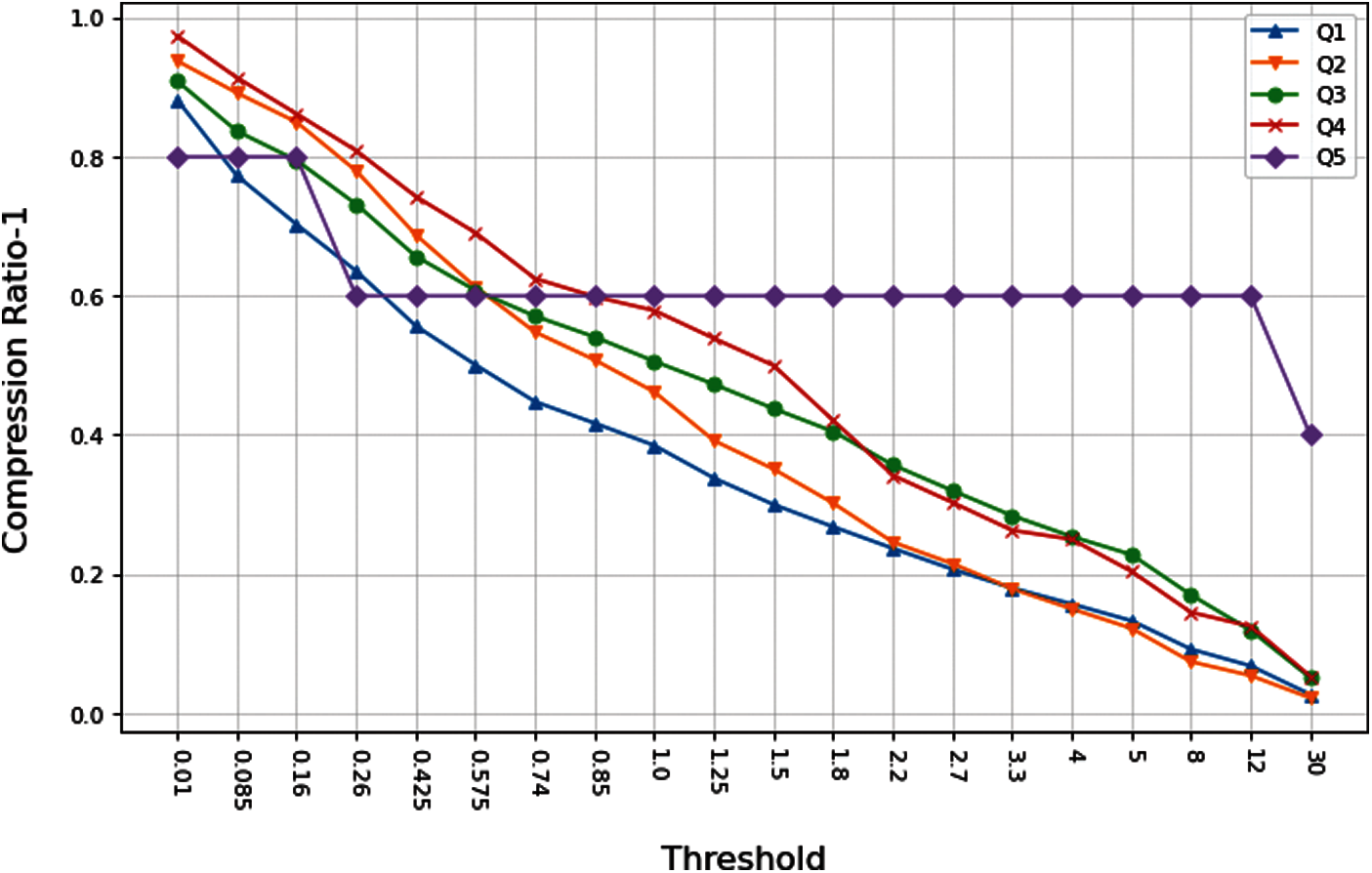
Figure 9: The relationship between threshold value and compression ratio under the DP algorithm

4.4 Performances Comparison

4.4.1 Performances of PED and SVE under DP Algorithm

The DP algorithm uses PED as the criterion for split points, thus it retains PED information greatly in trajectory compression. To demonstrate the well performance of the SVE under the DP algorithm, the variation rules of the PED and the SVE are analyzed experimentally with compression ratio of 150 trajectory segments. Fig. 10 shows the trend of the SVE with compression ratio from the Q1 to Q4. The abscissa indicates the reciprocal of the compression ratio while the ordinate indicates the error. In Fig. 10a, when c takes the maximum value of 100, the average PED of each point reaches 26.23 m. In this case, the average SVE error in latitude, i.e., LAT, is 1.95 m/s and the average SVE error in longitude, i.e., LON, is 2.14 m/s. When c takes the minimum value of 1.13, the average PED of each point is only 0.0005 m while the average LAT and LON is respectively 0.054 and 0.039 m/s. Similarly, Figs. 10b–10d have the same variation trends. Comparing the four figures, we can summarize three rules.

R3: The error of the trajectory points gradually increases as the compression ratio increases.

R4: The SVE fluctuates less than the PED under the DP algorithm.

R5: The average LAT and LON have similar growth trends and the gap gradually decreases as the data scale increases.

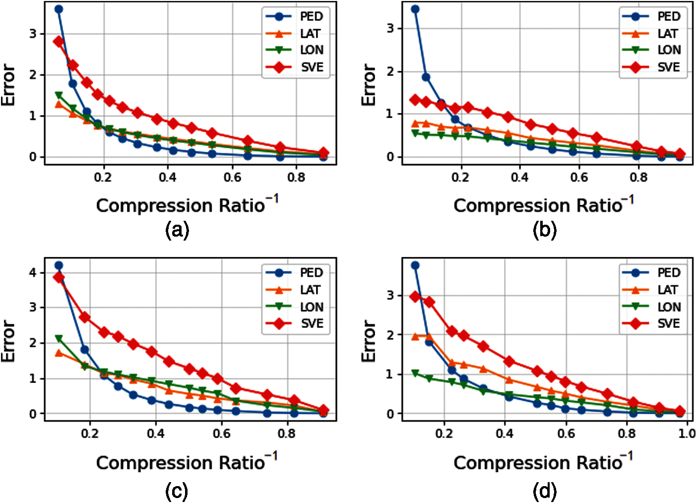
Figure 10: Trends of the SVE and the PED with compression rate from Q1 to Q4 under the DP algorithm. (a) Q1; (b) Q2; (c) Q3; (d) Q4

Fig. 11a shows the trends of the SVE and the PED with compression rate for 150 segment trajectories under the DP algorithm. The abscissa is the reciprocal of the compression ratio while the ordinate shows the average error between the compression and the raw trajectory. c−1 takes an arithmetic progression between 0.04 and 0.21 with interval of 0.01. As shown in Fig. 11a, the trajectory error in each interval is averaged and plotted between 0.045 and 0.205. When c−1 takes the value of 0.045, the average PED for each point is 10 m. In this case, the average SVE in latitude and longitude is 2.5 and 2.1 m/s, respectively. When c−1 takes the value of 0.205, the average PED for each point is 1.2 m. The average SVE in latitude and longitude are 1.3 and 1.0 m/s, respectively. To avoid the influence of the values on the growth trend, we scale the values in Fig. 11a by calculating the formula (38):

Ei′=EiE0.405, (38)

where Ei denotes the error value corresponding to the current compression ratio i and Ei′ denotes the error value after unitization.

As shown in Fig. 11b, the maximum error takes 1 when c−1 is 0.045 and the subsequent error is divided by the maximum error in turn. As shown in the figure, we can obviously find the following two rules:

R6: Under the DP algorithm, using the PED as the error criterion, the plot is parabolic as the compression ratio is gradually increased;

R7: Under the DP algorithm, the SVE has more linear characteristics compared to the PED.

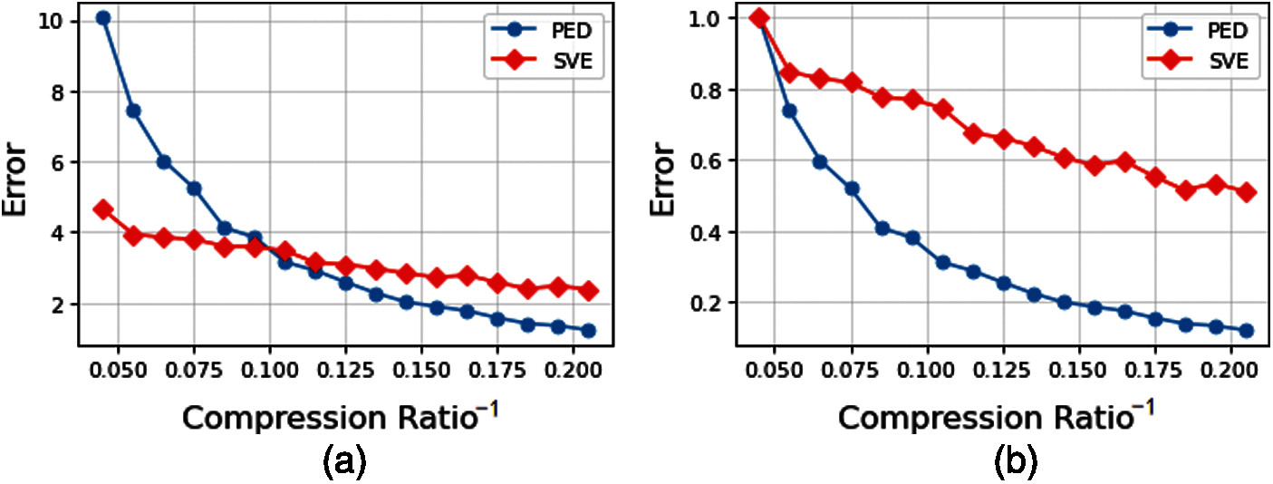
Figure 11: Trends of the SVE and the PED with compression rate for 150 segment trajectories under the DP algorithm. (a) Original error comparison; (b) Error comparison after standardization

In the subsequent experiments, we follow the operational procedure of the DP algorithm, so the repeated operations will not be described below.

4.4.2 Performances of SED and SVE under TD-TR Algorithm

The TD-TR algorithm uses the SED as the criterion for split points, thus it retains SED information greatly in the trajectory compression. To verify the well performance of the SVE under the TD-TR algorithm, the variation rules of the SED and the SVE are analyzed experimentally with compression ratio of 150 trajectory segments. Fig. 12 shows the trend of the SVE with compression ratio from the Q1 to Q4. The abscissa indicates the reciprocal of the compression ratio while the ordinate indicates the resulting error. In the Fig. 12a, when c takes the maximum value of 111, the average PED of each point reaches 60.96 m. In this case, the average LAT and LON for each point is respectively 1.48 and 1.58 m/s. By observing Fig. 12, we can find that the experimental results under the TD-TR algorithm still conform to the rules R3 and R5. In addition, we find the rule R8.

R8: The SVE in the TD-TR algorithm has a smaller variation of error compared to the SED.

Fig. 13a shows the trends of the SVE and the SED with compression rate for 150 segment trajectories under the TD-TR algorithm. When c−1 takes the value of 0.045, the average SED for each point reaches 34.16 m while the average SVE in latitude and longitude is 2.12 and 2.5 m/s, respectively. When c−1 takes the value of 0.205, the average SED is only 3.43 m while the average SVE in latitude and longitude is 1.08 and 1.29 m/s, respectively. In Fig. 13b, we find the rules R9 and R10.

R9: Under the TD-TR algorithm, using the SED as the error criterion, the plot is parabolic as the compression ratio is gradually increased.

R10: Under the TD-TR algorithm, the SVE evaluation criterion has more linear characteristics compared to the SED.

4.4.3 Performances of PED, SED and SVE under SW Algorithm

To demonstrate the performances of the PED, the SED and the SVE under the SW algorithm, the variation rules of each evaluation method are analyzed experimentally with compression ratio of 150 trajectory segments. Fig. 14 shows the trends of the SED, the PED, and the SVE with compression ratio from the Q1 to Q4. The abscissa indicates the reciprocal of the compression ratio while the ordinate indicates the error. In Fig. 14a, the PED and the SED show a massive increase when the compression ratio is small. At a compression ratio of 111.11, the average PED for each point is up to 132 m and the SED is up to 422 m, which is seriously unsuitable as an evaluation criterion. It performs similarly in Figs. 14b–14d. In contrast, the SVE performs well, with the average LAT and LON of 3.63 and 2.80 m/s respectively, which has no large-scale variations.

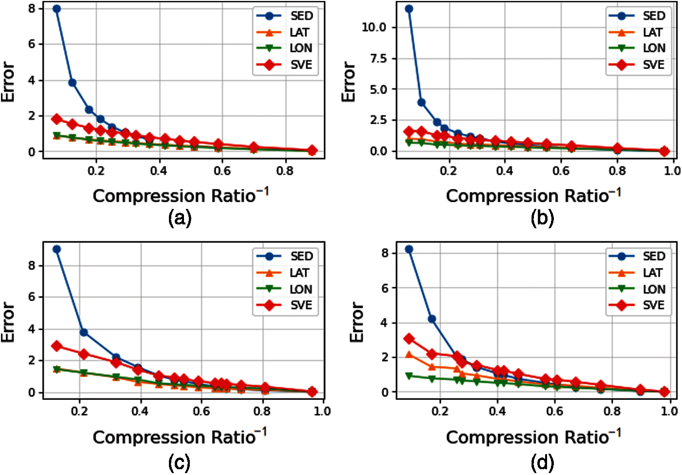
Figure 12: Trends of the SED and the SVE with compression rate from Q1 to Q4 under the TD-TR algorithm. (a) Q1; (b) Q2; (c) Q3; (d) Q4

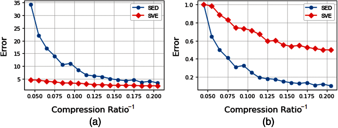
Figure 13: Trends of the SVE and the SED with compression rate for 150 segment trajectories under the TD-TR algorithm. (a) Original error comparison; (b) Error comparison after standardization

In the SW algorithm, when c takes the maximum value of 90.9, the average SED of each point reaches 80.75 m and the average PED is 23.57 m. In this case, the average SVE in latitude and longitude is 2.14 and 1.81 m/s, respectively. As shown in Fig. 15b, we can find the rules R11 and R12.

R11: Under the SW algorithm, the SED and the PED vary greatly as the compression ratio increases.

R12: Under the SW algorithm, the SVE has more linear characteristics compared to the PED and the SED.

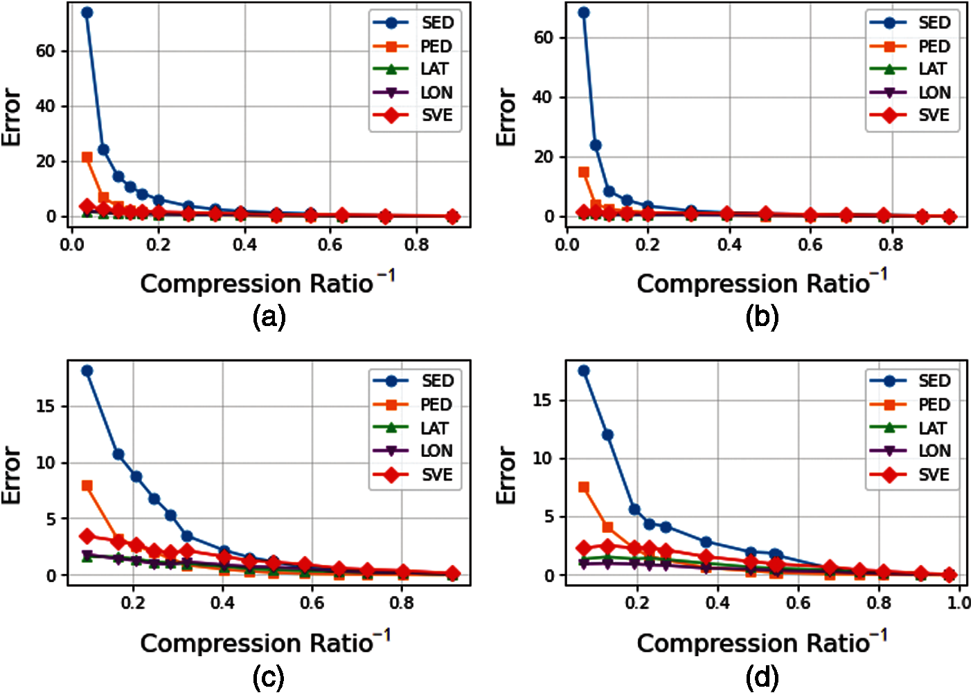
Figure 14: Trends of the SVE, the PED and the SED with compression rate from Q1 to Q4 under the SW algorithm. (a) Q1; (b) Q2; (c) Q3; (d) Q4

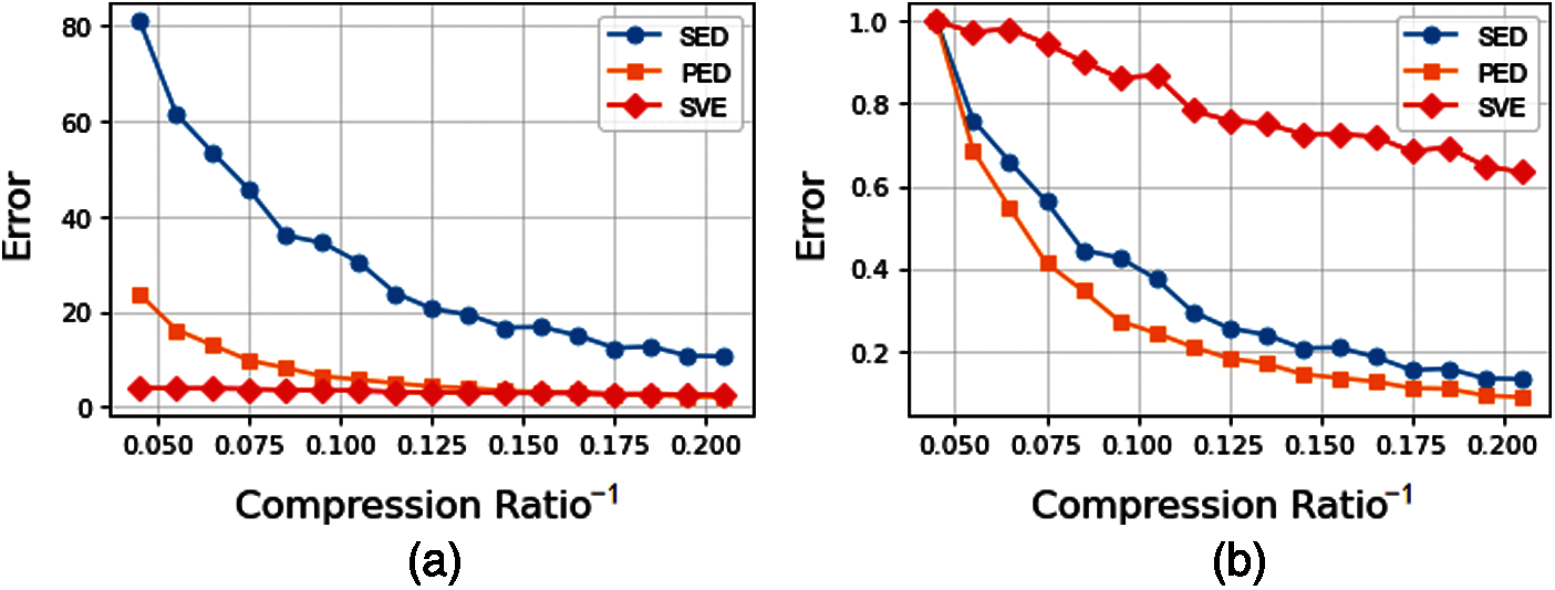
Figure 15: Trends of the SVE, the SED and the SED with compression rate for 150 segment trajectories under the SW algorithm. (a) Original error comparison; (b) Error comparison after standardization

4.4.4 Performances of PED, SED and SVE under SW-MSVE Algorithm

To demonstrate the performances of the PED, the SED and the SVE under the SW-MSVE algorithm, the variation rules of each evaluation method are analyzed experimentally with compression ratio of 150 trajectory segments. Fig. 16 shows the trends of the SED, the PED and the SVE with compression ratio from the Q1 to Q4 trajectory. The abscissa indicates the reciprocal of the compression ratio while the ordinate indicates the error. In the Fig. 16a, the PED and the SED show a massive growth when the compression ratio is small. At a compression ratio of 142.85, the average PED for each point is up to 418.67 m and the SED is up to 693.70 m, which is seriously unsuitable as an evaluation criterion. It performs similarly in Figs. 16b–16d. In contrast, the SVE performs well, with the average LAT and LON of 4.19 and 5.87 m/s respectively, which has no large-scale variations.

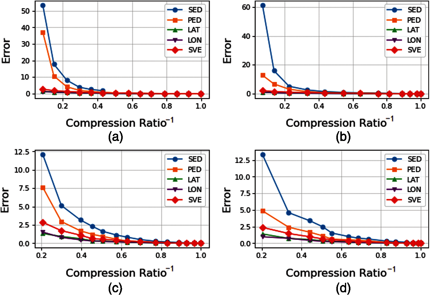
Figure 16: Trends of the SVE, the PED and the SED with compression rate from Q1 to Q4 under the SW-MSVE algorithm. (a) Q1; (b) Q2; (c) Q3; (d) Q4

In the SW-MSVE algorithm, when c takes the maximum value of 90.9, the average SED of each point reaches 168.95 m and the average PED is 74.16 m. In this case, the average SVE in latitude and longitude is 3.01 and 2.03 m/s, respectively. As shown in Fig. 17b, we can find the rules R13 and R14.

R13: Under the SW-MSVE algorithm, the SED and the PED vary greatly as the compression ratio increases.

R14: Under the SW-MSVE algorithm, the SVE has more linear characteristics compared to the PED and the SED.

4.4.5 Information Retention Rate of the Four Algorithms

Fig. 18 shows the raw trajectory map of the Q1 under the user 000. The activity range of the movable object is 39.900 to 40.075 N and 116.25 to 116.60 E (Beijing city) and a total of 14184 trajectory sequence points are recorded. In order to verify that the SW-MSVE algorithm retains more information in the trajectory compression, the experiment marks the points carrying larger PED, SED, and SVE information in the raw trajectory. The trajectories are compressed using the above four algorithms to test the information rate of their retaining. The experiments mark 3000 (about 25%) trajectory points in Q1. When c is 29.4, the retained PED, SED and SVE information by each algorithm is shown in Figs. 19–21, respectively. In general, the above algorithms can keep the geometric structure of the trajectory well. The definition of The Retention Rate is given below:

Retention Rate=NPMP×100 (39)

where MP denotes the number of marked points, NP denotes the number of the intersection of compressed points and marked points.

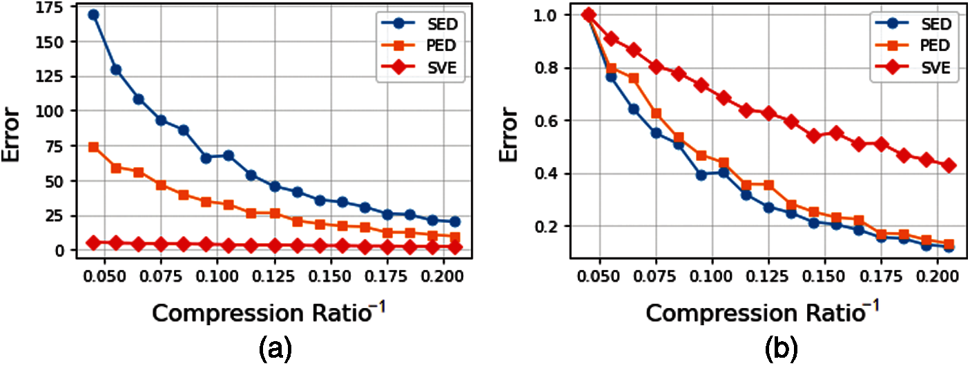
Figure 17: Trends of the SVE, the SED and the SED with compression rate for 150 segment trajectories under the SW-MSVE algorithm. (a) Original error comparison; (b) Error comparison after standardization

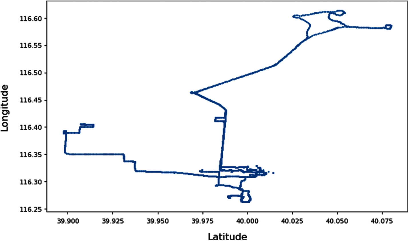
Figure 18: A section of the raw trajectory of user 000

The retained PED information of each trajectory compression algorithm is shown in Fig. 19. The red trajectory points are the PED marked points and the blue points are the non-PED marked points. According to the retention amount of PED information, the algorithm is sorted and the order from high to low is DP, SW, SW-MSVE and TD-TR. The DP and SW algorithms use the PED as the distance criterion of compression, thus to preserve more PED information in the compression. The PED information retention rate of the SW-MSVE algorithm is higher than that of the TD-TR algorithm, indicating that the SW-MSVE algorithm takes better account of the spatial geometric structure of the raw trajectory than the TD-TR algorithm.

The retained SED information of each trajectory compression algorithm is shown in Fig. 20. The red trajectory points are the SED marked points and the blue points are the non-SED marked points. According to the retention amount of SED information, the algorithm is sorted and the order from high to low is TD-TR, SW, SW-MSVE and DP algorithm. The TD-TR algorithm uses SED as the distance criterion, thus to preserve more SED information in the compression. The SED information retention ratio of the SW and SW-MSVE algorithms are very similar, indicating that the SW and SW-MSVE algorithms have similar ability to constrain the raw trajectories in both spatial and temporal dimensions. The DP has the weakest constraint ability.

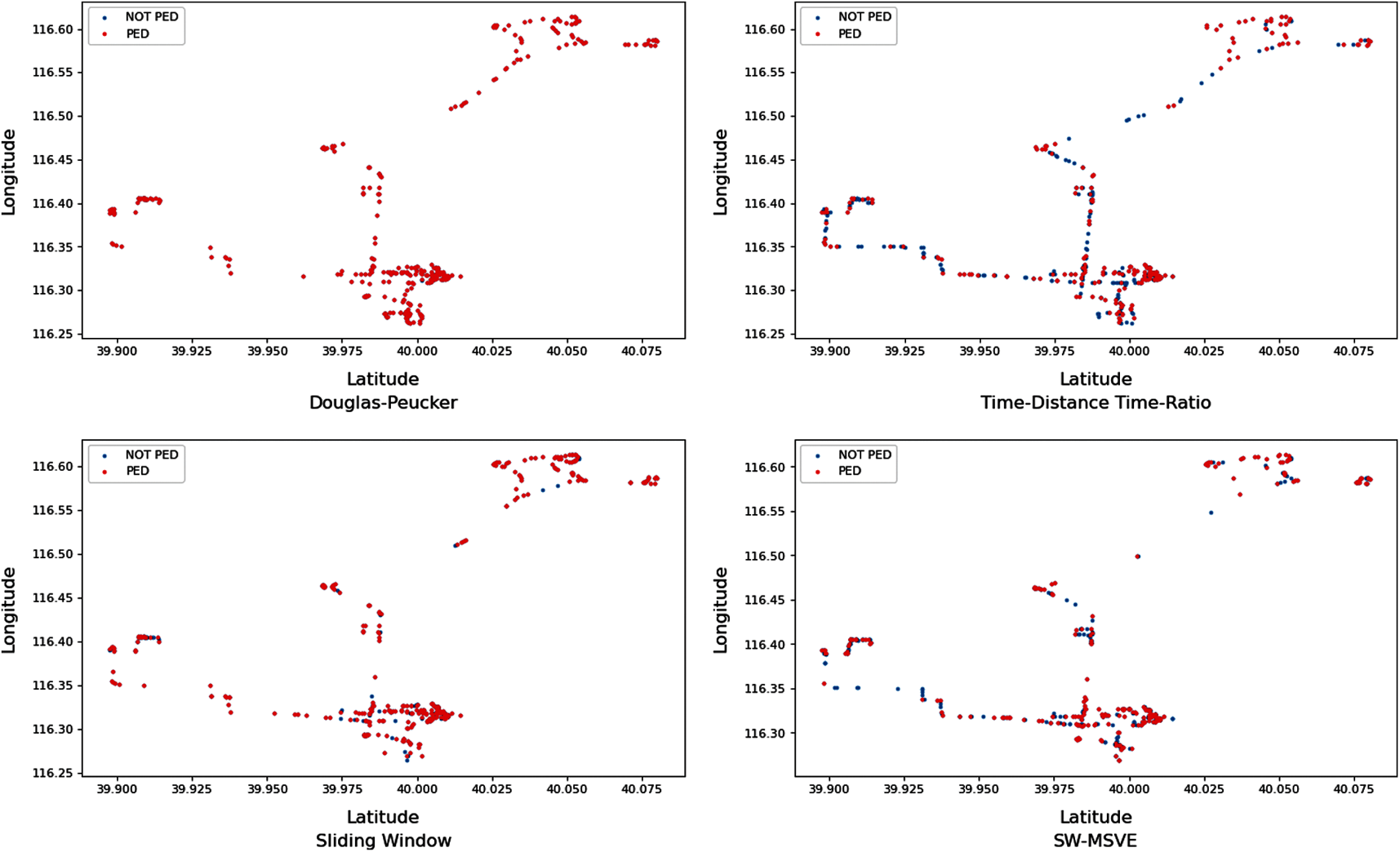
Figure 19: The PED information retention rate of the Q1 under the above four compression algorithms

The retained SVE information of each trajectory compression algorithm is shown in Fig. 21. The red trajectory points are the SVE marked points and the blue trajectory points are the non-SVE marked points. According to the retention amount of SVE information, the algorithm is sorted and the order from high to low is SW-MSVE, SW, TD-TR and DP algorithm. The SW-MSVE algorithm uses SVE as the distance criterion, thus to preserve more SVE information in the compression. The SW algorithm retains more SVE information than that of the TD-TR and DP algorithms, indicating that the SW algorithm takes better account of the velocity.

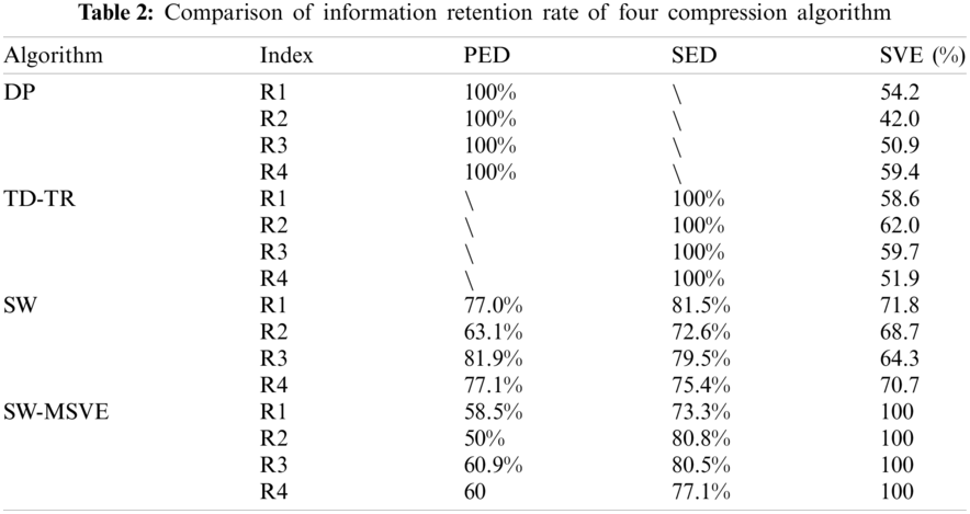
In order to further verify the above rules, four large-scale trajectories R1, R2, R3 and R4 are selected for the experiments. The experimental results are shown in Table 2. The experiments marked 3000 (about 25%) maximum PED, SED, and SVE points in R1 and 1250 (about 25%) maximum PED, SED, and SVE points in R2, R3 and R4, respectively. In the case of c = 29.4, it is recorded that the percentage of marked points in the compressed trajectory.

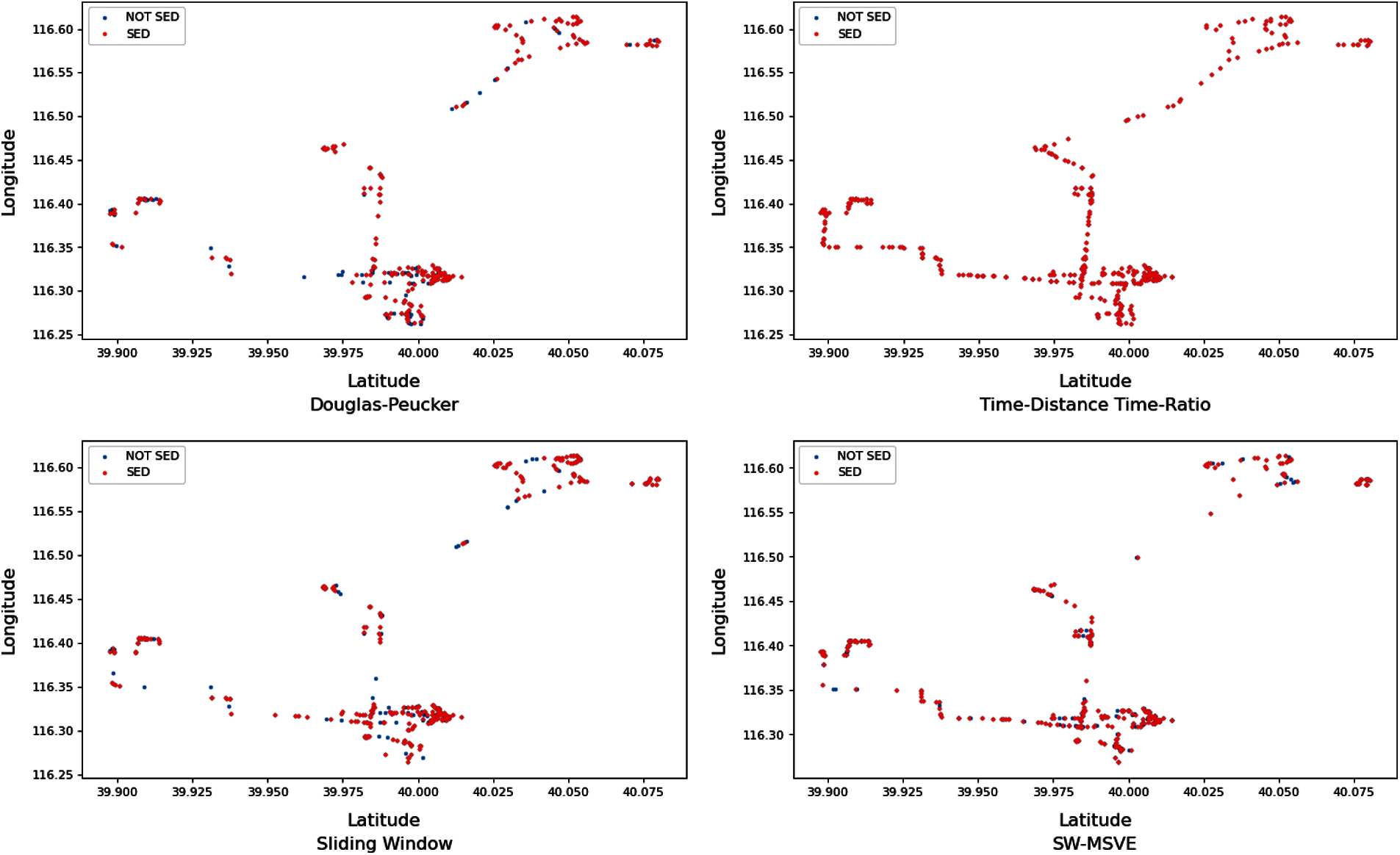
Figure 20: The SED information retention rate of the Q1 under the above four compression algorithms

Table 2 shows that the DP algorithm has poor performance in SVE that the information retention rate of is less than 60%, while the PED information retention rate under the SW-MSVE algorithm is higher than the DP algorithm. The TD-TR algorithm has higher information retention rate than the DP algorithm in the SVE, but it is far lower than the SED information retention rate in the SW-MSVE algorithm. The PED information retention rate under the SW algorithm is higher than the SW-MSVE algorithm and their SED information retention rate are almost the same and the SVE information retention rate is kept at only 70%. The overall information retention rate of the SW algorithm is slightly lower than that of the SW-MSVE algorithm. In general, the SW-MSVE algorithm has highest information retention rate than the other algorithms.

5  Discussion

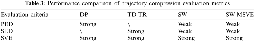
During the above experiments, we analyze the four algorithms of trajectory compression using the SVE, the PED, and the SED, respectively. The experimental results are shown in Table 3. At the same algorithm, the SVE varies less than the PED and the SED when the compression ratio gradually increases. This situation indicates that the SVE has better adaptability than the PED and the SED. When we use the PED and the SED to evaluate the error of trajectory with high compression rate, there will be many abnormal values. The SVE will not have such a situation. When using the PED and the SED to evaluate the Sliding Window algorithm, the error greatly fluctuates and the quality of trajectory compression cannot be accurately evaluated, so the performance is weaker. Similarly, the rest of the performance is recorded in the table. When we use the SVE to measure the error of four algorithms, the experiments show that they are less influenced by noise and the overall variation has linear characteristics with stronger performance and more applicability.

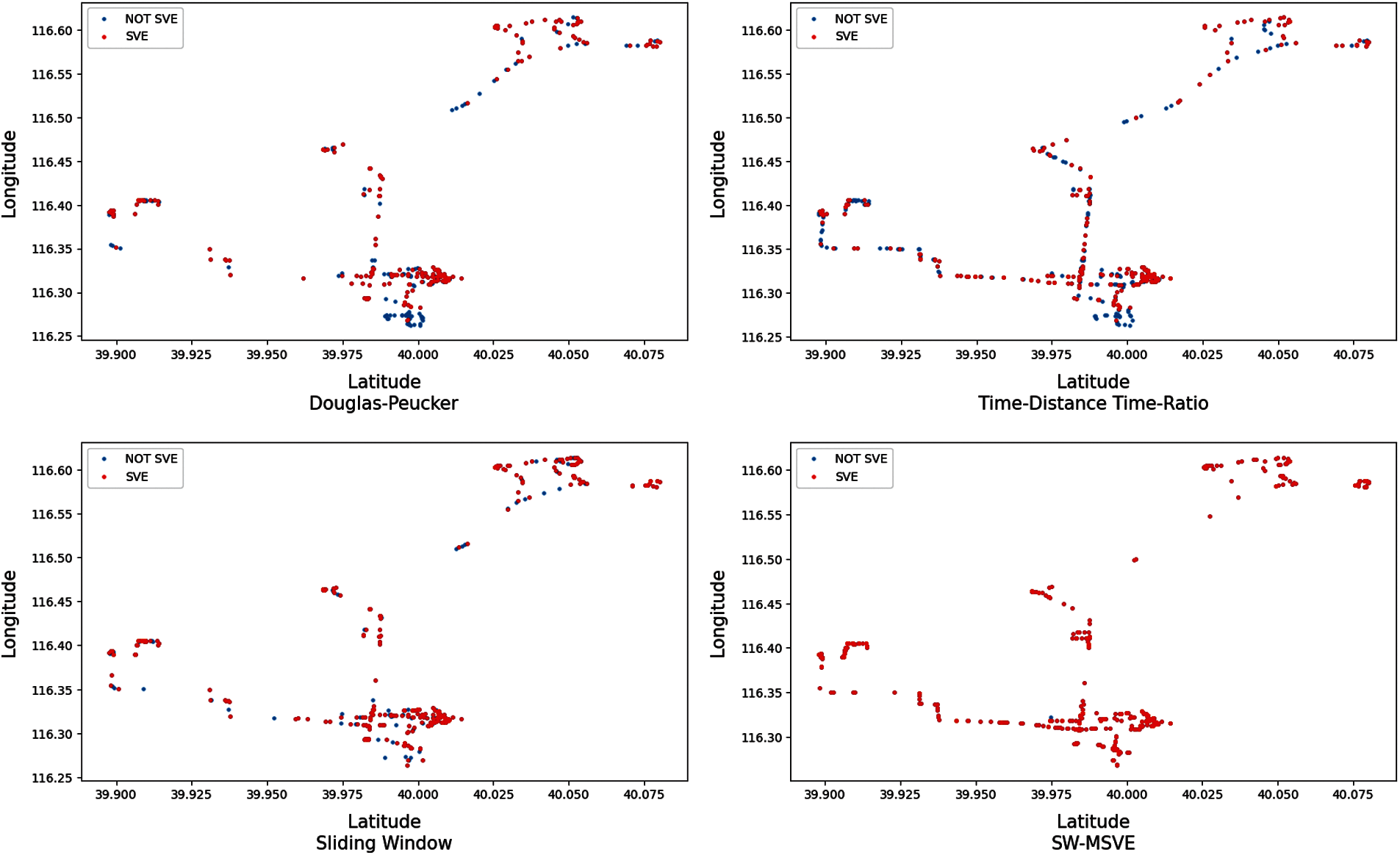
Figure 21: The PED information retention rate of the Q1 under the above four compression algorithms

For the SW-MSVE algorithm, the quality in the trajectory compression is experimentally demonstrated. In this process, the SW-MSVE always retains higher information rate compared to the DP and TD-TR algorithms. For example, while retaining 100% of the SVE information points, the algorithm retains up to 80.8% PED information points. The SW-MSVE algorithm has low time complexity and is applicable to both offline and online compression methods.

6  Conclusions

In this paper, a new evaluation model (SVE) of trajectory compression error is proposed and its feasibility is verified experimentally, which fills the gap on evaluation of velocity error for trajectory compression in industry. This model is less influenced by noise and has linear characteristics in the overall variation with strong performance, so that it can be applied to more algorithms. Base on this model, an innovative trajectory compression algorithm (SW-MSVE) is proposed in this paper. The SW-MSVE algorithm uses the time synchronous velocity error as the distance function, which retains more valuable information of the raw trajectory in the compression. This algorithm provides a new idea for the trajectory compression method because the lower time complexity and wider applicability. In the future research, we believe that there will be more and more researches based on the SVE which will be widely applied in fields gradually. But there are still some shortcomings in the algorithms and models. For example, there are some bumpy shapes to appear in figure when we use the SVE to evaluate some trajectory segments in the experiment. These shortcomings may be caused by the lack of accurate filtering before trajectory compression. In future experiments, the constraints on trajectory filtering should be strengthened to avoid the influence of noise points. Besides, the current SW-MSVE algorithm can only guarantee the minimized overall velocity error with local optimization therefore in the future work we should design more reliable algorithms can minimize the global velocity error. The SVE model and the SW-MSVE algorithm are mainly constrained for velocity and thus are more suitable for which applications with high constraints on velocity.

Acknowledgement: The authors would like to thank the Assistant Editor of this article and anonymous reviewers for their valuable suggestions and comments.

Funding Statement: This research is supported by the National Natural Science Foundation of China under Grants 61873160 and 61672338.

Conflicts of Interest: The authors declare that they have no conflicts of interest to report regarding the present study.

This work is licensed under a Creative Commons Attribution 4.0 International License, which permits unrestricted use, distribution, and reproduction in any medium, provided the original work is properly cited.