Computer Modeling in Engineering & Sciences

DOI: 10.32604/cmes.2022.018267

ARTICLE

Sine Trigonometry Operational Laws for Complex Neutrosophic Sets and Their Aggregation Operators in Material Selection

D. Ajay1, J. Aldring1, G. Rajchakit2, P. Hammachukiattikul3 and N. Boonsatit4,*

1Sacred Heart College (Autonomous), Tamil Nadu, 635601, India
2Maejo University, Chiang Mai, 50290, Thailand
3Phuket Rajabhat University, Phuket, 83000, Thailand
4Rajamangala University of Technology Suvarnabhumi, Nonthaburi, 11000, Thailand
*Corresponding Author: N. Boonsatit. Email: nattakan.b@rmutsb.ac.th
Received: 11 July 2021; Accepted: 07 September 2021

1  Introduction

One of the complex problems in all types of industries/companies is making decisions based on ambiguous information. As a consequence, the concept of fuzzy set theory has been employed to deal with this type of situation or problem. Zadeh [1] first proposed the concept of fuzzy subsets in 1965. It has sparked numerous significant outcomes in the scientific community, which have been replicated in modern applications, particularly in decision-making and artificial intelligence. In addition, different researchers have extended the core idea of fuzzy sets to handle different types of uncertainty, and the extended notions of fuzzy sets include intuitionistic fuzzy sets (IFSs) [2], Pythagorean fuzzy sets (PFSs) [3], Fermatean fuzzy sets (FFSs) [4], Neutrosophic sets (NSs) [5], and Spherical fuzzy sets (SFSs) [6] among others and each of them addresses the problem of uncertainty in a unique way. Based on these notions, various multi criteria decision making (MCDM) approaches are available in the literature like weighted sum method (WSM), weighted product method (WPM), the multiple criteria optimization compromise solution (VIKOR), the technique for order performance by similarity to the ideal solution (TOPSIS), the Weighted Aggregates Sum Product Assessment (WASPAS), COmbinative Distance-Based ASsessment (CODAS), and the Evaluation Based on Distance from Average Solution (EDAS), etc., MCDM is a technique for selecting the best option from a set of alternatives and neutrosophic sets have found wide scope in such techniques. Edalatpanah established a new model of data envelopment analysis based on triangular neutrosophic numbers [7]. And also neutrosophic approach have been implemented to data envelopment analysis with undesirable outputs by Mao et al. [8]. A new ranking function of triangular neutrosophic number [9] and systems of neutrosophic linear equations are introduced by Edalatpanah [10].

Complex fuzzy sets (CFSs) are a significant research area of investigation in fuzzy logic. It was proposed by Ramot et al. [11,12]. CFSs use a complex membership function to handle uncertainty with periodicity which takes complex values within the complex unit circle. Clearly, the complex memership function of a CFS comprises two terms named amplitude term and phase term which lie in the intervals and , respectively. The phase term accounts for the periodicity of the data and distinguishes CFSs from the traditional models of fuzzy set theory. CFSs and Complex Fuzzy Logic (CFL) have been utilized to develop accurate and efficient time series forecasting models [13,14], image processing [15], etc. The concept of CFSs, has been further extended to complex intuitionistic fuzzy sets (CIFSs) [16], complex Pythagorean fuzzy sets (CPFSs) [17], complex neutrosophic sets (CNSs) [18] and so on and also it is evident from the literature that notable research have been carried out in complex fuzzy sets scenario. Recently, Xu et al. [19] introduced an extended EDAS method with a single-valued complex neutrosophic set and its application in green supplier selection. Complex neutrosophic generalized dice similarity measures have been developed by Ali et al. [20]. Also, another MCDM model called a soft set based VIKOR is developed based on CNSs by Manna et al. [21]. Some of complex hybrid weighted averaging operators are introduced for decision making in [22]. Aggregating the fuzzy information plays an important role in decision theory and it is involved in majority of MCDM methods.

In addition operational laws also play a vital role in aggregation process. Also it is evident from the literature that various operational laws are available. Gou et al. [23] used new type of operational laws for IFSs. Then, Li et al. [24] introduced the logarithmic operational laws for IFSs in order to aggregate information. Later, Garg et al. [25] introduced a new logarithmic operational laws for single valued neutrosophic number which yields application in multi attribute decision making. Also, Ashraf et al. [26] used logarithmic hybrid aggregation operators for single valued neutrosophic sets. In continuation, Garg et al. [27] have presented some new exponential, logarithmic, and compensative exponential of logarithmic operational laws for complex intuitionistic fuzzy (CIF) numbers based on t-norm and co-norm. Garg also utilized the logarithmic operational laws for PFSs in [28]. Further, Nguyen et al. [29] developed exponential similarity measures for Pythagorean fuzzy sets and their application in pattern recognition. Haque et al. [30] utilized exponential operational laws for generalized SFSs. Another novel concept of neutrality operational laws have been introduced by Garg et al. [31] for q-rung orthopair fuzzy sets and Pythagorean fuzzy geometric aggregation operators [32]. Also, Garg extended the new exponential operation laws for q-rung orthopair fuzzy sets in [33].

Sine trigonometric operational laws were introduced by Garg [34]. The main advantage of sine trigonometric function is that it accounts for the periodicity and it is symmetric about the origin. Thus it satisfies the expectations of the decision-maker over the multi-time phase parameters. Garg [35] introduced a novel trigonometric operation based q-rung ortho pair fuzzy aggregation operators and he also extended these operational laws to Pythagorean fuzzy information [36]. Abdullah et al. [37] developed an approach of ST-OLs for picture fuzzy sets. Ashraf et al. [38] utilized the concept of single valued neutrosophic sine trigonometric aggregation operators for hydrogen power plant selection and further they implemented these operational laws for spherical fuzzy environment in [39]. MCDM methods namely TOPSIS and VIKOR have been developed based on ST-OLs by Qiyas et al. [40,41]. From the literature, it is clear that ST-OLs play predominant role in aggregation operators (AOs). Through this motivation and considering the advantage of ST-OLs, some new ST-OLs for CNSs must be established and their behaviour in complex scenario needs to be studied. Hence, this paper aims to modify sine trigonometric operational laws for complex neutrosophic sets and implement them in complex decision making method for material selection. So, the main objective of this paper can be described as follows:

(i). To present the ST-OLs for CNSs

(ii). To obtain some of the distance measure for complex neutrosophic sets based on ST-OLs

(iii). To develop an MCDM technique with the help of the proposed aggregation operators

(iv). To demonstrate an entropy technique based on ST-OLs for CNNs in order to attain complex weights of criteria

(v). To give an application of the proposed MCDM method in material selection in an industry

(vi). Finally, to present the validation of the developed method with existing CODAS approach

The organization of the paper is the following; We review the basic concept of NSs in the second section of the paper. In Section 3, we explore the operations of enhanced ST-OLs for NSs. These ST-OLs have been extended to CNSs in Section 4, including subtraction and distance measurement of ST-OLs for CNSs. In Section 5, we develop AOs and prove their properties for ST-OLs of CNSs. In Section 6, an MCDM approach has been explained in detailed steps with entropy technique for criteria weights. The proposed MCDM approach is used to provide an application for material selection in Section 7. The validation and discussion of the study is carried out in Section 8. Finally, the paper is concluded in Section 9 with direction for further research.

2  Preliminaries

Some of the basic concepts of neutrosophic sets (NSs) with their operations are discussed here.

Definition 2.1 [1] A fuzzy set defined on a universe of discourse has the form: where . Here denotes the membership function of each .

Definition 2.2 [2] An intuitionistic fuzzy set is defined as a set of ordered pairs over a universal set and is given by where with the condition for each element . Here the membership and non-membership functions are denoted as and , respectively.

Definition 2.3 [5] Let be a universe of discourse or a non empty set. Any object in the neutrosophic set has the form , where , and represent the degree of truth membership, the degree of indeterminacy and the degree of false membership respectively of each element to the set and it is defined as where such that .

Definition 2.4 [5] Let , and be three neutrosophic numbers (NNs) and let be any scalar. Then

Definition 2.5 Let and be two NNs. Then

i. if and only if , , for each

ii. if and only if and

Definition 2.6 Let , and be three NNs. Then the score and accuracy functions of NNs are defined as follows:

(1)

(2)

Also, the following conditions hold good.

(1) If then

(2) If then

(3) If then

(4) If then

(5) If then

(6) If then

3  Sine Trigonometry Operational Law (STOL) for Neutrosophic Sets

First, the STOL [34] are applied to neutrosophic sets and the boundary conditions are verified.

Definition 3.1 Let the neutrosophic numbers (NNs) be . Then, the sine trigonometric operational laws of NNs are defined as follows:

(1)

From the above STOL of NNs, it is evident that the is also NNs. And it satisfies the following condition of neutrosophic set as the degree of truth, indeterminacy, and falsity of NS are defined, respectively

such that

,

such that ,

such that ,

Also, . Therefore, STOL of NNs are also NNs, a fact which is also affirmed by Fig. 1.

Then we discuss the fundamental operations on sine trigonometric neutrosophic numbers (STNNs) and their properties.

Figure 1: This is a graph of STOLs of NNs

Definition 3.2 Let , and be neutrosophic numbers (NNs) and let be any scalar. Then

•   Complement of :

•   Intersection of and :

•   Union of and :

•   Algebric sum of and :

•   Algebric product of and :

•   Scalar product of :

•   Power of :

Definition 3.3 Let and be two sine trigonometric neutrosophic numbers. Then

i.    if and only if , , for each

ii.    if and only if and

Definition 3.4 Let be a neutrosophic number. Then the score and accuracy functions of STOL of NNs are defined as follows:

1.    

2.    

Here the score and accuracy range values of STOLs of NNs are discussed in pictorial representation in the following Figs. 2 and 3 when the membership values of , , are equal.

Figure 2: This is a graph of score range values of STOLs of NNs

Figure 3: This is a graph of accuracy range values of STOLs of NNs

4  Sine Trigonometry Operational Laws (STOLs) for Complex Neutrosophic Sets (CNSs)

First, we see some basic concepts of complex neutrosophic sets and their operations.

Definition 4.1 [18] A complex neutrosophic set , is represented by truth membership function , an indererminacy membership function and a falsity membership function that take complex values for any . The three membership values and their sum may all lie within the unit circle in the complex plane and this is of the following form: where and are amplitude terms whose values lie in , and the phase terms are such that and . The modulus of is , also denoted by . Similarly, the modulus of are , respectively. The set builder form of the complex neutrosophic set is represented as where, such that

.

Example 4.1 Let be a universe of discourse. Then, is a complex neutrosophic set in given by

4.1 The STOLs of CNSs

The STOLs have been introduced for complex neutrosophic sets and their boundary conditions are verified.

Definition 4.2 Let be a complex neutrosophic number (CNN).

Then, the sine trigonometric operational law of CNNs (ST-OLs-CNNs) is defined as follows:

(2)

From the above STOL of CNNs, it is evident that the is also a CNN. And it satisfies the following condition of CNSs as the degree of truth, indeterminacy, and false of complex neutrosophic sets are defined, respectively.

Also,

Example 4.2 Let be a complex neutrosophic number (CNN).

Then, the sine trigonometric operational law of CNNs (ST-OLs-CNNs) is also a CNN. We describe the function as follows:

(3)

Also, the modulus of ST-OLs of CNNs is listed below and it is observed that the sum of values is less than or equal to three.

Then we discuss the fundamental operations on sine trigonometric operational laws of CNNs and their properties.

Definition 4.3 [18] Let , , be three neutrosophic numbers (NNs) and let be any scalar.

Then the sine operational laws of , and are described below:

• Complement of :

• Intersection of and :

• Union of and :

• Algebric sum of and :

• Scalar product of :

• Algebric product of and :

• Power of :

Definition 4.4 Let be sine trigonometric operational law of CNN.

Then, score and accuracy of are also CNNs and they are defined as follows:

(4)

(5)

Next, the properties of sine trigonometric operational laws of CNNs are discussed.

Theorem 4.1 Let and be two ST-OL-CNNs. Then,

•   

•   

Proof. The proofs are straightforward from the Definition 4.3.

Theorem 4.2 Let and be two ST-OL-CNNs and . Then,

(i).

(ii).

(iii).

(iv).

(v).

Proof. Let and be two ST-OL-CNNs;

Then, using Definition 4.3 the algebraic sum of two ST-OL-CNNs

(i). For any , then we have

Hence the property (i) is proved.

The proof of property (ii). is similar

(iii). For any , we have

Hence the proof of property (iii).

Theorem 4.3 Let and be two ST-OL-CNNs such that , , and , , . Then .

Proof. For any two CNNs

Similarly, for indeterminacy and falsity membership functions.

Hence we get from the Definition 4.2 that

4.2 Subtraction of Two Sine Trigonometric CNNs

Definition 4.5 Let ; be two sine trigonometric CNNs mentioned as follows:

The subtraction is defined as

(6)

Example 4.3 Let two sine trigonometric CNNs be

Then the subtraction is calculated as follows:

(7)

4.3 Distance Measure of ST-OL-CNNs

In this section, we discuss different types of distance measures of ST-OL-CNNs.

•   Let , be two collections of ST-OL-CNNs. Then the Minkowski distance (MD) measure between two ST-OL-CNNs is defined as follows:

(8)

•   When in Eq. (8), it is called the Manhattan distance measure

•   Similarly, when Eq. (8), is called the Euclidean distance measure.

Example 4.4 Let ST-OLs for two CNNs be given by

Then, the distance measures are

• Manhattan distance measure (Ma-D):

• Euclidean distance measure (ED):

• Minkowski distance measure (MD) when :

Note: Here the subtraction of two ST-OL-CNNs is calculated using Eq. (6).

The Minkowski distance measures of ST-OL-CNNs satisfies the following properties:

(i).

(ii). ; that means

(iii).

(iv). If is a ST-OL-CNNs in and if , then and

5  Aggregation Operators for ST-OLs-CNSs

In this section, the weighted averaging and geometric aggregation operators are presented for ST-OLs-CNNs with numerical example.

5.1 Sine Trigonometry Weighted Averaging Aggregation Operator (ST-WAAO)

Definition 5.1 Let be complex neutrosophic numbers (CNNs).

Then the ST-WAAOs for CNNs is denoted by and defined as follows:

(9)

where represents the weights of such that and .

Theorem 5.1 Let be CNNs and the weights of be such that and . Then the is defined as follows:

(10)

Proof. The proof of Theorem 5.1 is examined by mathematical induction on n. For each P, be CNNs.

Step I. For , we get

Using Definition 4.3, the algebraic sum of two ST-OL-CNNs is a CNN. Therefore, is also a CNN. Further,

Step II. Suppose that Eq. (10) holds for ,

Step III. Next, we have to prove that Eq. (10) holds for ,

Hence the proof.

Example 5.1 Suppose that , , are CNNs and the corresponding weights are given respectively as . Then the value of is calculated as follows:

Then absolute value of ST-WAAO-CNN is calculated as follows:

Next, we give some properties of the ST-WAAO-CNNs operator and establish that they preserve idempotency, boundedness, monotonically, and symmetry.

Theorem 5.2 Let be CNNs such that . Then

Proof. Let . By Theroem 5.1, we get

Hence proved.

Theorem 5.3 Let be CNNs and

Then,

Proof. For any P,

This implies that . Suppose that , and . Then, based on the monotonicity of sine function, we have

similarly,

Also, we have

similarly,

Then, Therefore, .

Theorem 5.4 Let and be two collections of CNNs.

If , ,

, then

Proof. It follows from Theorem 5.3 and hence the proof is omitted.

Theorem 5.5 Let and be two collections of CNNs. Then whenever is any version of .

Proof. The proof follows from Theorem 5.3.

5.2 Sine Trigonometry Weighted Geometric Aggregation Operator (ST-WGAO)

Definition 5.2 Let be complex neutrosophic numbers (CNNs).

Then the ST-WGAOs for CNNs is denoted by and defined as follows:

(11)

where represents the weights of such that and .

Theorem 5.6 Let be CNNs and the weights of be represented by such that and . Then the is defined as follows:

(12)

Proof. The proof of theorem 5.6 is examined by mathematical induction on n. For each P, be CNNs. Then the following steps are involved.

Step I. For , we get

Using Definition 4.3, the algebraic product of two ST-OL-CNNs is a CNN. Therefore, is also a CNNs. Further,

Step II. Suppose that Eq. (12) holds for ,

Step III. Next, we have to prove the Eq. (12) holds for ,

Hence the proof.

Example 5.2 Let , , be CNNs and the corresponding weights are given respectively as . Then the value of is calculated as follows:

Then absolute value of ST-WGAO-CNN is calculated as follows:

Theorem 5.7 Let be CNNs such that . Then

Theorem 5.8 Let be CNNs and

Then,

Theorem 5.9 Let and be two collections of CNNs.

If , , , then

Theorem 5.10 Let and be two collections of CNNs. Then whenever is any version of .

The proof of above all theorems 5.7–5.10 follow from Theorems 5.2–5.5 directly.

5.3 Fundamental Properties of ST-AOs for CNNs

Theorem 5.11 Let and are two collections of CNNs. Then we have

Proof. Since and be two collection of CNNs. By Definition 4.3

As for any , .

Thus, by taking , , we have

Similarly,

Therefore,

Theorem 5.12 Let be CNNs and for any ,

1.    

2.    

Proof. The proof of the theorem follows from Theorem 5.11.

Theorem 5.13 Let be CNNs, then

Here the equality holds if and only if

Proof. The proof of the theorem follows from Theorem 5.11.

6  Decision Making Techniques

This section presents a decision making technique that could be utilized to solve uncertain multi criteria decision making (MCDM) problems with complex neutrosophic information. MCDM problems can be handled by decision matrix, in which all elements are represented in terms of ST-OLs-CNNs with respect to alternatives over criteria/attributes by decision makers. Thus, a decision matrix , consists of n number of alternatives and m number of criteria/attributes . The unknown weight vector of each criterion is denoted by which could be calculated by entropy method.

Suppose that the complex neutrosophic decision matrix (ST-Ols-CNDM) is denoted by ,

where all elements are ST-OLs-CNNs , . The decision making algorithm is described in the following steps:

Step 1. The collected vague data are transformed to ST-OLs-CNNs

Step 2. Construct the normalized complex neutrosophic decision matrix from ,

where is computed by the following conditions

If is benefit type criteria/attributes

If is cost type criteria/attributes

Step 3. The weights of the criteria/attributes are unknown. So the entropy principle 6.1 is used to calculate the weights of criteria/attributes .

Step 4. From the normalized decision matrix and the criteria weight vector , the fused information of each alternative are obtained by either ST-WAAO-CNN (Eq. (10)) or ST-WGAO-CNN (Eq. (12)).

Step 5. Calculate the score value of each aggregated value.

Step 6. Rank the alternatives according to their absolute score values.

6.1 Entropy Method

Shannon proposed the theory of entropy [42], which is a measure of uncertainty in information represented in terms of probability theory. To evaluate relative weights, Shannon's entropy approach interprets the relative intensities of the criterion based on the discrimination among data. The steps in the shannon's entropy approach are as follows:

Step (i). The complex neutrosophic decision matrix is formed:

Step (ii). Utilize score function to initial ST-Ols-CN decision matrix and find secondary score decision matrix where the elements are complex fuzzy numbers

Step (iii). Then, normalize the secondary decision matrix

Step (iv). Calculate the entropy of each criterion

Step (v). Calculate the variation coefficient of criterion

Step (vi). Determine the weight of each criterion by the following equation:

(13)

7  Application of the Proposed ST-OLs-Complex Neutrosophic Decision Making Approach

The selection of materials for industry plays an essential role in their functioning. Also, the growing material availability in the world has created a variety of options. But, very less attention has been given to tools and methods that facilitate material selection process. In addition, this process needs to consider multiple properties depending on tools/method requirements to make a better decision. For manufacturers and engineers, it is a crucial and challenging task to select best sustainable option from a number of materials used in the modern industry and many factors are involved in such decision making process. MCDM approaches are more efficient in the selection process of materials. Khandekar et al. [43] utilized decision making approach based on fuzzy axiomatic design principles for material selection. Mayyas et al. [44] implemented fuzzy TOPSIS method to select best eco-material. A fuzzy logic based PROMETHEE method have been used for material selection problems by Gul et al. [45]. Using TOPSIS approach with some popular normalization methods Yang et al. [46] proposed an efficient method for material selection. A systematic review on material selection methods have been explained in detail by Rahim et al. [47].

Case Study. A manufacturing company is planning to buy materials from suppliers based on four criteria namely -Cost, -Quality and efficiency of the material, -Demand, -Availability of the material. Usually in the complex neutrosophic numbers, the amplitude values lie between zero and one that represent the initial intuition values of material over criteria and the phase terms represent the secondary intuition values after a certain interval of time. Through this process, a decision maker evaluates the alternatives (Materials) under these criteria and gives his preference values in CNNs which are given in Tables 1 and 2. Then the weights of criteria are calculated based on entropy approach and demonstrated numerically in the following Subsection 7.1:

Step 1. The formation of ST-OLs-complex neutrosophic decision matrix that is Table 2 is derived from usual complex neutrosophic decision matrix (Table 1).

Step 2. All the criteria are benefit type. The normalized ST-OLs of complex neutrosophic decision matrix is taken from Table 2.

Step 3. The weights of the criteria/attributes are unknown. So the entropy principle 6.1 has been used to calculate the following weights of criteria/attributes.

Step 4. From the normalized decision matrix , i.e., Table 2 and the criteria weight vector , the fused information of each alternative are obtained obtained using ST-WAAO-CNN (Eq. (10)) and given in Table 3.

Step 5. The score values of each alternative are given below:

Step 6. The ranking order of the alternatives according to their amplitude values is listed as follows:

Therefore, .

Similarly, Using ST-WGAO-CNN (Eq. (12)) operator, the aggregated complex neutrosophic decision matrix is obtained and is shown in Table 4;

The score value of each alternative are given below:

The ranking order of the alternatives according to their amplitude values is listed as follows:

Then, the ranking order is .

7.1 Calculation of Entropy Based Criteria Weights

These are the following steps involved in the Shannon's entropy method to calculate the criteria weights;

Step (i). The initial complex neutrosophic decision matrix is considered from Table 2.

Step (ii). Using score function to initial ST-Ols-CN decision matrix , we get the secondary score decision matrix where all elements are complex fuzzy numbers as mentioned in Table 5.

Step (iii). The normalization of the secondary decision matrix is given in Table 6.

Step (iv). The entropy of each criterion is given as follows: where,

Step (v). The variation coefficient of each criterion is calculated by . The values are

Step (vi). Finally, the weight of each criterion are calculated using Eq. (13)

Note: The result satisfies the property that the sum of all complex weights is equal to one. That means

8  Validation of the Proposed Method

The proposed concept of sine trigonometry operational laws of complex neutrosophic decision making approach is verified with entropy based combinative distance-based assessment (CODAS) method. A decision matrix, i.e., Table 2 has been taken for entropy-CODAS method. In the initial process, criteria weights are derived using the steps given in Section 6.1. And the weight values are calculated and given as follows; The steps of entropy based CODAS method as mentioned in the literature by Ghorabaee et al. [48] is demonstrated numerically for ST-OLs-CNNs as follows:

Step 1. The ST-OLs-CN decision-making matrix is considered as in Table 2

Step 2. Each element in ST-OLs-CN decision matrix is normalized by the following linear normalization Eq. (14)

(14)

Step 3. The ST-OLs-CN weighted normalized decision matrix is calculated by , where denotes the complex weights of each criterion such that .

Step 4. The ST-OLs-CN negative-ideal solution of the weighted normalized decision matrix is given in Table 7.

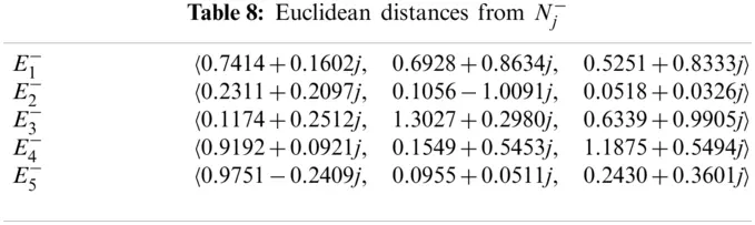
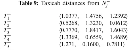
Step 5. The Euclidean and Taxicab distances of alternatives from the ST-OLs-CN negative-ideal solution are calculated by Eqs. (15) and (16)

(15)

(16)

The values are shown in Tables 8 and 9.

Step 6. The relative assessment of ST-OLs-CN matrix is derived from Eq. (17), and shown as in Table 10.

(17)

where denotes a threshold function used to recognize the equality of the Euclidean distances of two alternatives, and is defined as follows:

(18)

is the threshold parameter that can be set by decision-maker. It is better that this parameter be a value between 0.01 and 0.05. Here, the value is 0.01.

Step 7. The assessment value of each alternative is obtained by Eq. (19)

(19)

Step 8. Using ST-OLs-CN score function, the score of each is calculated as follows:

Step 9. Rank the alternatives according to the absolute values

8.1 Discussion and Comparison Analysis

The outcomes of the new and existing techniques are compared in Table 12 to demonstrate the validity of the proposed approach. It is transparent that the optimal alternative is the same for all techniques. As a result, the proposed concept of sine trigonometric operational laws of complex neutrosophic sets performs better in complex decision-making procedures. But, this operator can handle only the particular types of uncertainty which have periodicity in the form of amplitude and phase terms to the three membership functions such as truth, indeterminacy and falsity where amplitude represents the real valued membership functions and an additional term called phase represents periodicity. In this research, the execution of multi-criteria decision making approach their results in complex numbers. So, in order to select the best among them we have to consider the absolute values.

9  Conclusion

In this study, a decision making method with sine trigonometric operational laws for complex neutrosophic fuzzy sets have been proposed. The operations of ST-OLs-CNNs play a vital role during the decision making process and with help of these operations some of the ST-OLs-CN aggregation operators have been developed in order to make decision over complex vague information. The description of ST-OLs have been given with CNNs in detailed graphical representation and it shows the validity of the ST-OLs. The properties of the proposed sine trigonometric weighted AOs are proved. Further, in the proposed MCDM method, the criteria weights are computed by unsupervised techniques and by combining these methods a new approach called Entropy-ST-OLs-CNDM method has been introduced. Then the functionality of the proposed method is applied to a material selection problem and, feasibility and validity of the approach are investigated in detail with comparative analysis.

In future research, advanced study of the similarity measures of complex neutrosophic sets and complex neutrosophic critic-based approach for handling MCDM problems with unknown weights can be carried out. The recommended approach can also be applied to other fields, such as medical nutrition diagnostics, sustainable supplier selection, and so on.

Funding Statement: This work was supported in part by the Rajamangala University of Technology Suvarnabhumi.

Conflicts of Interest: The authors declare that they have no conflicts of interest to report regarding the present study.

References

 1.  Zadeh, L. (1965). Fuzzy sets. Information and Control, 8, 338–353. DOI 10.1016/S0019-9958(65)90241-X. [Google Scholar] [CrossRef]

 2.  Atanassov, K. (1983). Intuitionistic fuzzy sets. Fuzzy Sets and Systems, 20, 87–96. DOI 10.1016/S0165-0114(86)80034-3. [Google Scholar] [CrossRef]

 3.  Yager, R. (2013). Pythagorean fuzzy subsets. Joint IFSA World Congress and NAFIPS Annual Meeting, pp. 57–61. DOI 10.1109/IFSA-NAFIPS.2013.6608375. [Google Scholar] [CrossRef]

 4.  Senapati, T., Yager, R. (2020). Fermatean fuzzy sets. Journal of Ambient Intelligence and Humanized Computing, 11, 663–674. DOI 10.1007/s12652-019-01377-0. [Google Scholar] [CrossRef]

 5.  Samrandache, F. (1999). A unifying field in logics. In: Neutrosophy: Neutrosophic probability, set and logic. Rehoboth: American Research Press. [Google Scholar]

 6.  Gündogdu, F., Kahraman, C. (2019). Spherical fuzzy sets and spherical fuzzy topsis method. Journal of Intelligent & Fuzzy Systems, 36, 337–352. DOI 10.3233/JIFS-181401. [Google Scholar] [CrossRef]

 7.  Edalatpanah, S. A. (2020). Data envelopment analysis based on triangular neutrosophic numbers. CAAI Transactions on Intelligence Technology, 5, 94–98. DOI 10.1049/trit.2020.0016. [Google Scholar] [CrossRef]

 8.  Mao, X., Zhao, G. X., Fallah, M., Edalatpanah, S. A. (2020). A neutrosophic-based approach in data envelopment analysis with undesirable outputs. Mathematical Problems in Engineering, 2020, 1–8. DOI 10.1155/2020/7626102. [Google Scholar] [CrossRef]

 9.  Kumar Das, S., Edalatpanah, S. A. et al. (2020). A new ranking function of triangular neutrosophic number and its application in integer programming. International Journal of Neutrosophic Science, 4(2), 82–92. DOI 10.5281/zenodo.3767107. [Google Scholar] [CrossRef]

10. Edalatpanah, S. A. (2020). Systems of neutrosophic linear equations. Neutrosophic Sets and Systems, 33, 6. DOI 10.5281/zenodo.3782826. [Google Scholar] [CrossRef]

11. Ramot, D., Milo, R., Friedman, M., Kandel, A. (2002). Complex fuzzy sets. IEEE Transactions on Fuzzy Systems, 10, 171–186. DOI 10.1109/91.995119. [Google Scholar] [CrossRef]

12. Ramot, D., Friedman, M., Langholz, G., Kandel, A. (2003). Complex fuzzy logic. IEEE Transactions on Fuzzy Systems, 11, 450–461. DOI 10.1109/TFUZZ.2003.814832. [Google Scholar] [CrossRef]

13. Ma, J., Zhang, G., Lu, J. (2012). A method for multiple periodic factor prediction problems using complex fuzzy sets. IEEE Transactions on Fuzzy Systems, 20, 32–45. DOI 10.1109/TFUZZ.2011.2164084. [Google Scholar] [CrossRef]

14. Li, C., Chiang, T. W. (2012). Intelligent financial time series forecasting: A complex neuro-fuzzy approach with multi-swarm intelligence. International Journal of Applied Mathematics and Computer Science, 22, 787–800. DOI 10.2478/v10006-012-0058-x. [Google Scholar] [CrossRef]

15. Li, C., Wu, T., Chan, F. (2012). Self-learning complex neuro-fuzzy system with complex fuzzy sets and its application to adaptive image noise canceling. Neurocomputing, 94, 121–139. DOI 10.1016/j.neucom.2012.04.011. [Google Scholar] [CrossRef]

16. Alkouri, A. M. J. S., Salleh, A. R. (2012). Complex intuitionistic fuzzy sets. AIP Conference Proceedings, 1482(1), 464–470. DOI 10.1063/1.4757515. [Google Scholar] [CrossRef]

17. Ullah, K., Mahmood, T., Ali, Z., Jan, N. (2020). On some distance measures of complex pythagorean fuzzy sets and their applications in pattern recognition. Complex & Intelligent Systems, 6, 15–27. DOI 10.1007/s40747-019-0103-6. [Google Scholar] [CrossRef]

18. Ali, M., Smarandache, F. (2015). Complex neutrosophic set. Neural Computing and Applications, 28, 1817–1834. DOI 10.1007/s00521-015-2154-y. [Google Scholar] [CrossRef]

19. Xu, D., Cui, X., Xian, H. (2020). An extended edas method with a single-valued complex neutrosophic set and its application in green supplier selection. Mathematics, 8(2), 282. DOI 10.3390/math8020282. [Google Scholar] [CrossRef]

20. Ali, Z., Mahmood, T. (2020). Complex neutrosophic generalised dice similarity measures and their application to decision making. CAAI Transactions on Intelligence Technology, 5, 78–87. DOI 10.1049/trit.2019.0084. [Google Scholar] [CrossRef]

21. Manna, S., Basu, T. M., Mondal, S. (2020). A soft set based vikor approach for some decision-making problems under complex neutrosophic environment. Engineering Applications of Artificial Intelligence, 89, 103432. DOI 10.1016/j.engappai.2019.103432. [Google Scholar] [CrossRef]

22. Li, D., Mahmood, T., Ali, Z., Dong, Y. (2020). Decision making based on interval-valued complex single-valued neutrosophic hesitant fuzzy generalized hybrid weighted averaging operators. Journal of Intelligent & Fuzzy Systems, 38, 4359–4401. DOI 10.3233/JIFS-191005. [Google Scholar] [CrossRef]

23. Gou, X., Xu, Z., Lei, Q. (2016). New operational laws and aggregation method of intuitionistic fuzzy information. Journal of Intelligent & Fuzzy Systems, 30, 129–141. DOI 10.3233/IFS-151739. [Google Scholar] [CrossRef]

24. Li, Z., Wei, F. (2017). The logarithmic operational laws of intuitionistic fuzzy sets and intuitionistic fuzzy numbers. Journal of Intelligent & Fuzzy Systems, 33, 3241–3253. DOI 10.3233/JIFS-161736. [Google Scholar] [CrossRef]

25. Garg, H., Nancy (2018). New logarithmic operational laws and their applications to multiattribute decision making for single-valued neutrosophic numbers. Cognitive Systems Research, 52, 931–946. DOI 10.1016/j.cogsys.2018.09.001. [Google Scholar] [CrossRef]

26. Ashraf, S., Abdullah, S., Smarandache, F., ul Amin, N. (2019). Logarithmic hybrid aggregation operators based on single valued neutrosophic sets and their applications in decision support systems. Symmetry, 11, 364. DOI 10.3390/sym11030364. [Google Scholar] [CrossRef]

27. Garg, H., Rani, D. (2019). Exponential, logarithmic and compensative generalized aggregation operators under complex intuitionistic fuzzy environment. Group Decision and Negotiation, 28, 991–1050. DOI 10.1007/s10726-019-09631-8. [Google Scholar] [CrossRef]

28. Garg, H. (2019). New logarithmic operational laws and their aggregation operators for pythagorean fuzzy set and their applications. International Journal of Intelligent Systems, 34, 106–82. DOI 10.1002/int.22043. [Google Scholar] [CrossRef]

29. Nguyen, X. T. N., Nguyen, V. D., Nguyen, V., Garg, H. (2019). Exponential similarity measures for pythagorean fuzzy sets and their applications to pattern recognition and decision-making process. Complex & Intelligent Systems, 5, 217–228. DOI 10.1007/s40747-019-0105-4. [Google Scholar] [CrossRef]

30. Haque, T., Chakraborty, A., Mondal, S., Alam, S. (2020). Approach to solve multi-criteria group decision-making problems by exponential operational law in generalised spherical fuzzy environment. CAAI Transactions on Intelligence Technology, 5, 106–114. DOI 10.1049/trit.2019.0078. [Google Scholar] [CrossRef]

31. Garg, H., Chen, S. M. (2020). Multiattribute group decision making based on neutrality aggregation operators of q-rung orthopair fuzzy sets. Information Sciences, 517, 427–447. DOI 10.1016/j.ins.2019.11.035. [Google Scholar] [CrossRef]

32. Garg, H. (2019). Novel neutrality operation based pythagorean fuzzy geometric aggregation operators for multiple attribute group decision analysis. International Journal of Intelligent Systems, 34, 2459–2489. DOI 10.1002/int.22157. [Google Scholar] [CrossRef]

33. Garg, H. (2021). New exponential operation laws and operators for interval-valued q-rung orthopair fuzzy sets in group decision making process. Neural Computing and Applications, 33, 1–27. DOI 10.1007/s00521-021-06036-0. [Google Scholar] [CrossRef]

34. Garg, H. (2020). Decision making analysis based on sine trigonometric operational laws for single-valued neutrosophic sets and their applications. Applied and Computational Mathematics, 19, 255–276. [Google Scholar]

35. Garg, H. (2020). A novel trigonometric operation-based q-rung orthopair fuzzy aggregation operator and its fundamental properties. Neural Computing and Applications, 32, 1–23. DOI 10.1007/s00521-020-04859-x. [Google Scholar] [CrossRef]

36. Garg, H. (2021). Sine trigonometric operational laws and its based pythagorean fuzzy aggregation operators for group decision-making process. Artificial Intelligence Review, 54, 4421–4447. DOI 10.1007/s10462-021-10002-6. [Google Scholar] [CrossRef]

37. Abdullah, S., Khan, S., Qiyas, M., Chinram, R. (2021). A novel approach based on sine trigonometric picture fuzzy aggregation operators and their application in decision support system. Journal of Mathematics, 2021, 1–19. DOI 10.1155/2021/8819517. [Google Scholar] [CrossRef]

38. Ashraf, S., Abdullah, S., Zeng, S., Jin, H., Ghani, F. (2020). Fuzzy decision support modeling for hydrogen power plant selection based on single valued neutrosophic sine trigonometric aggregation operators. Symmetry, 12, 298. DOI 10.3390/sym12020298. [Google Scholar] [CrossRef]

39. Ashraf, S., Abdullah, S. (2021). Decision aid modeling based on sine trigonometric spherical fuzzy aggregation information. Soft Computing, 25, 8549–8572. DOI 10.1007/s00500-021-05712-6. [Google Scholar] [CrossRef]

40. Qiyas, M., Abdullah, S., Khan, S., Naeem, M. (2021). Multi-attribute group decision making based on sine trigonometric spherical fuzzy aggregation operators. Granular Computing, 6, 1–22. DOI 10.1007/s41066-021-00256-4. [Google Scholar] [CrossRef]

41. Qiyas, M., Abdullah, S. (2021). Sine trigonometric spherical fuzzy aggregation operators and their application in decision support system, topsis, vikor. The Korean Journal of Mathematics, 29, 137–167. DOI 10.11568/kjm.2021.29.1.137. [Google Scholar] [CrossRef]

42. Shannon, C. E. (2001). A mathematical theory of communication. ACM SIGMOBILE Mobile Computing and Communications Review, 5(1), 3–55. DOI 10.1145/584091.584093. [Google Scholar] [CrossRef]

43. Khandekar, A. V., Chakraborty, S. (2015). Decision-making for materials selection using fuzzy axiomatic design principles. International Journal of Industrial and Systems Engineering, 20, 117–138. DOI 10.1504/IJISE.2015.069003. [Google Scholar] [CrossRef]

44. Mayyas, A., Omar, M. A., Hayajneh, M. (2016). Eco-material selection using fuzzy topsis method. International Journal of Sustainable Engineering, 9, 292–304. DOI 10.1080/19397038.2016.1153168. [Google Scholar] [CrossRef]

45. Gul, M., Celik, E., Gumus, A. T., Guneri, A. F. (2018). A fuzzy logic based promethee method for material selection problems. Beni-Suef University Journal of Basic and Applied Sciences, 7, 68–79. DOI 10.1016/j.bjbas.2017.07.002. [Google Scholar] [CrossRef]

46. Yang, W. C., Chon, S. H., Choe, C. M., Yang, J. Y. (2021). Materials selection method using topsis with some popular normalization methods. Engineering Research Express, 3, 1–28. DOI 10.1088/2631-8695/abd5a7. [Google Scholar] [CrossRef]

47. Rahim, A., Musa, S., Ramesh, S., Lim, M. K. (2020). A systematic review on material selection methods. Proceedings of the Institution of Mechanical Engineers. Part L: Journal of Materials: Design and Applications, 234, 1032–1059. DOI 10.1177/1464420720916765. [Google Scholar] [CrossRef]

48. Ghorabaee, M. K., Zavadskas, E., Turskis, Z., Antucheviciene, J. (2016). A new combinative distance-based assessment (CODAS) method for multi-criteria decision-making. Economic Computation and Economic Cybernetics Studies and Research, 50, 25–44. [Google Scholar]

This work is licensed under a Creative Commons Attribution 4.0 International License, which permits unrestricted use, distribution, and reproduction in any medium, provided the original work is properly cited.