| Computer Modeling in Engineering & Sciences |
DOI: 10.32604/cmes.2022.018234
ARTICLE
Image Reconstruction for ECT under Compressed Sensing Framework Based on an Overcomplete Dictionary
1School of Electrical and Control Engineering, Xi’an University of Science and Technology, Xi’an, 710054, China
2Shaanxi Coal and Shaanbei Mining Co., Ltd., Xi’an, 719000, China
*Corresponding Author: Xuebin Qin. Email: qinxb@xust.edu.cn
Received: 09 July 2021; Accepted: 02 September 2021
Abstract: Electrical capacitance tomography (ECT) has great application potential in multiphase process monitoring, and its visualization results are of great significance for studying the changes in two-phase flow in closed environments. In this paper, compressed sensing (CS) theory based on dictionary learning is introduced to the inverse problem of ECT, and the K-SVD algorithm is used to learn the overcomplete dictionary to establish a nonlinear mapping between observed capacitance and sparse space. Because the trained overcomplete dictionary has the property to match few features of interest in the reconstructed image of ECT, it is not necessary to rely on the sparsity of coefficient vector to solve the nonlinear mapping as most algorithms based on CS theory. Two-phase flow distribution in a cylindrical pipe was modeled and simulated, and three variations without sparse constraint based on Landweber, Tikhonov, and Newton-Raphson algorithms were used to rapidly reconstruct a 2-D image.
Keywords: Electrical capacitance tomography; dictionary learning; compressed sensing; k-SVD algorithm; overcomplete dictionary; two-phase flow
In industrial processes, it is often necessary to analyze information about two-phase flow in a pipeline or closed container. Traditional detection methods have been unable to provide accurate measurement because of the complexity of flow motion. In recent decades, with the development of modern measurement technology, electrical tomography (ET), with its advantages of non-invasive, non-damaging characteristics, and simple structure and low cost, has attracted extensive attention from researchers. At present, ET mainly includes electrical resistance tomography [1] (ERT), electrical impedance tomography [2] (EIT), electromagnetic tomography [3] (EMT), and electrical capacitance tomography [4] (ECT). ECT investigated in this study is a technique for visualizing a two-phase medium with phases of different permittivity in a pipe or a closed container. The system is suitable for imaging multicomponent phase flows, such as sand, that are not conductors. ECT technology has shown great potential in many fields, such as multiphase flow measurement [5], combustion imaging [6], and solid particle monitoring in a fluidized bed [7,8].
The objective of ECT is to obtain projection data through a sensor array fixed on the outer wall of a pipe or container, and then use an algorithm to obtain the internal permittivity distribution, which is presented with 2-D or 3-D images. The sensor array is composed of multiple electrodes, and the number of electrodes can be 8, 12, or 16. The mutual capacitances between electrodes are collected to form a capacitance sequence which is the projected data reflecting internal information. Mathematical modeling computes the permittivity distribution from the capacitance sequence, which is an inverse problem model. Many algorithms have been proposed to solve the inverse problem, such as Convolutional Neural Networks (CNN), the linear inverse projection algorithm (LBP), Landweber algorithm, and Tikhonov regularization algorithm. Deep learning has shown great advantages in many fields, especially in image processing [9,10]. Deep learning has many advantages such as strong learning ability, wide coverage, and good portability [11–13]. However, deep learning models are more complex and time-consuming. High, it violates the real-time nature of electrical capacitance tomography. The LBP algorithm has fast computation but low image accuracy. The Landweber algorithm is a simple iterative algorithm, and many scholars have improved its convergence rate [14–16]. The inverse problem is ill-posed, but the Tikhonov regularization algorithm transforms the ill-posed problem into a well-posed problem by adding regularization constraint terms based on the l2-norm to the target function, and then obtains an effective solution. The reconstructed image is smooth but insensitive to edge contours.
Most algorithms establish approximate linear mapping to replace non-linear mapping because of the “soft field” in ECT, resulting in low accuracy of the reconstructed image. In 2006, Donoho proposed compressive sensing (CS) theory [17], which pointed out that when the signal is sparse or compressible, the original signal can be accurately reconstructed with far fewer samples than that required by Shannon’s theorem. In recent years, Figueiredo and Candes etal. extended CS theory [18–21]. CS theory has been widely applied in the field of imaging, and it can be used for image reconstruction in ECT [22–24].
In CS theory, the transform basis for sparse representation is crucial. For image reconstruction systems in different application fields, the transform basis is generally the specified orthogonal basis, such as discrete Fourier transform (DFT) [25], discrete cosine transform (DCT) [26], or discrete wavelet transform (DWT) [27]. The classical orthonormal basis is better for some features of the image but is negative for two-phase distributions, because two-phase flow is always varied in a complex industrial process. Specifying an orthonormal basis may reflect the permittivity distribution of a flow pattern such as stratified flow. To solve the above problems, this paper introduces the idea of CS and dictionary learning to ECT theory [28,29], which is called D-CS-ECT. Different flow patterns are used to train the transform basis so that it matches the different features of the permittivity distribution as much as possible to improve the accuracy of the reconstructed image [30].
In this paper, the transform basis is an overcomplete dictionary. The overcomplete dictionary is flexible and adaptive. It captures different features of the signal through multiple atoms and improves the redundancy of the transform system to approximate the original signal. There are some features of interest in the image reconstructed by ECT system, which focus on the position and boundary of the two phases. The trained overcomplete dictionary is able to match the features.
This paper is organized as follows: in Section2, the basic principles of ECT and CS theory based on over-complete dictionaries are introduced. In Section3, the process of dictionary learning is described, which is mainly the construction of a training sample set and the application of the K-SVD algorithm. The reconstruction results are analyzed and evaluated through simulation in Section4. Concluding remarks are presented in Section5.
2 ECT under the Framework of D-CS Theory
The hardware architecture of ECT systems is composed of a sensor array, data acquisition module, and image reconstruction unit. In this study, a sensor array with 12 electrodes is driven by an excitation voltage, as shown in Fig. 1b, and the electrodes are numbered from 1 to 12. Firstly, Electrode 1 is excited with a 1 V voltage while the other electrodes are grounded. The capacitance values between Electrode 1 and Electrodes 2, 3, 4
where N is the number of capacitor sequences, and M is the number of electrodes.
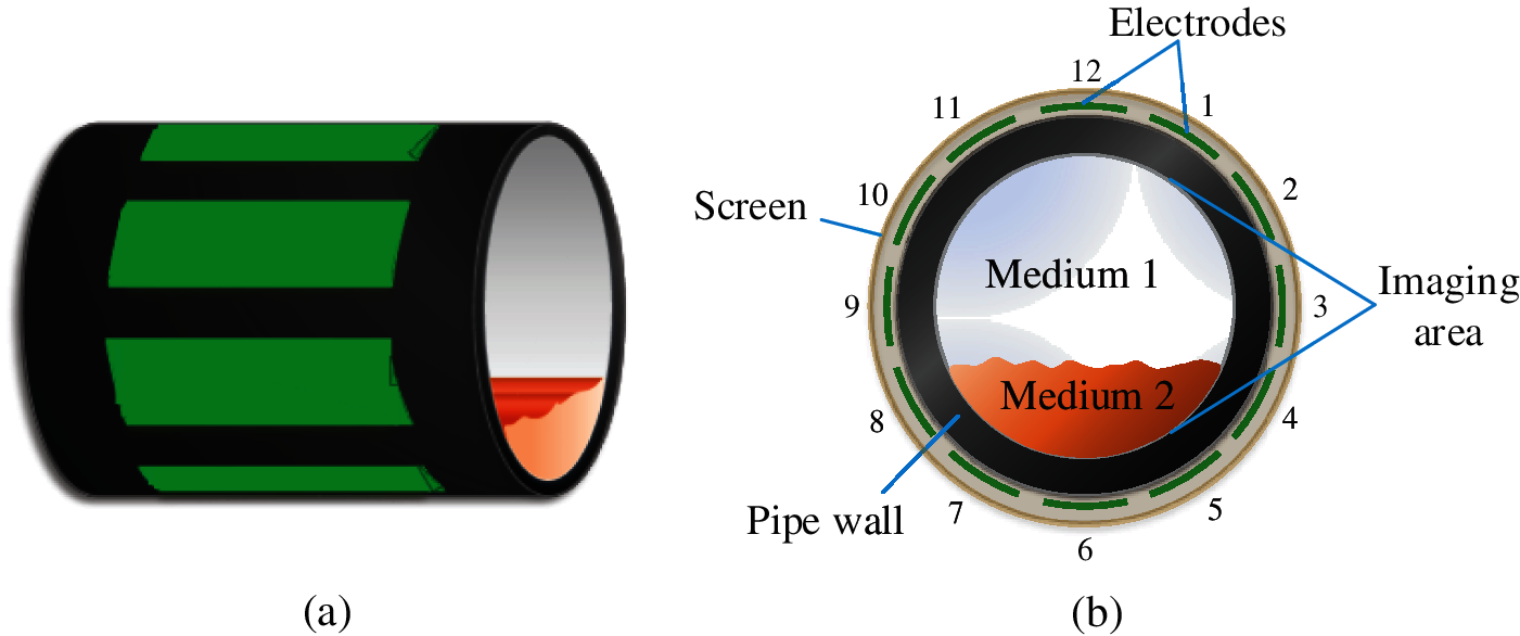
Figure 1: ECT sensor with 12 electrodes for two-phase flow in the pipeline. (a) 3-D structure; (b) 2-D section
For a complex and changeable two-phase flow, the distribution in the pipeline includes seven flow patterns: central bubble flow, eccentric bubble flow, two-bubble flow, three-bubble flow, four-bubble flow, stratified flow, and annular flow, as shown in Fig. 2.
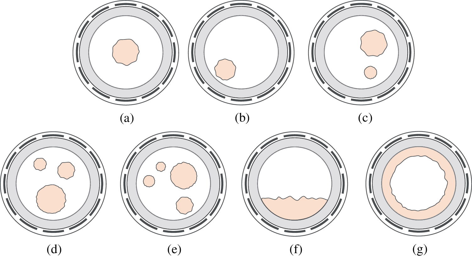
Figure 2: Different flow patterns. (a) Central bubble flow; (b) Eccentric bubble flow; (c) Two-bubble flow; (d) Three-bubble flow; (e) Four-bubble flow; (f) Stratified flow; (g) Annular flow
In ECT, the approximate linear relationship between the capacitance sequence and the permittivity sequence is described by the following equation:
where
In Fig. 1b,
where (3) is the parallel normalization method, and (4) is the series normalization method. It can be seen from (3) or (4) that the
S from (2) is the sensitivity matrix of the empty field state. According to the potential distribution in the imaging area [33], the discrete derivation result for S is
where the number of electrodes is M, the number of pixels distributed in the imaging area is n, and the excitation voltage of the electrode is U=1 V. Ci, j is the capacitance scalar between the i − th electrode and the j − th electrode. At the spatial position of the k − th pixel point,
The normalization method for the sensitivity matrix is given by
where
To obtain the image is to solve g. Because the number of the capacitance sequence obtained from the sensor is far lower than the number of pixels in the reconstructed image, S is an ill-posed matrix, and (2) is ill-posed and its solution is not unique. The error function is minimized in the inverse problem of the ECT, that is,
Many existing image reconstruction algorithms for ECT can be improved on the basis of (7), such as adding constraint terms based on the l2-norm to the target function.
CS theory mainly includes three parts: the sparse representation of signal, design of the observation matrix, and signal reconstruction. D-CS using a dictionary rather than an orthogonal basis is a branch of CS theory [34]. Proposed the dictionary-restricted isometry property (D-RIP), which is a natural generalization of the restricted isometry property (RIP) [35], proving that the idea of signal reconstruction by a redundant and coherent dictionary is feasible. The mathematical model for D-CS-ECT is given below.
The image signal is represented as a small number of values in sparse space through an overcomplete dictionary. Sparse representation can be expressed as
where
The nonlinear mapping relation between the observed capacitance and the coefficient vector can be written as
where
The procedure of the reconstruction algorithm is to first solve x according to (9), and then solve g according to (8). Classical signal reconstruction algorithms based on CS theory mainly include greedy algorithms and convex optimization algorithms. In this study, the sparsity adaptive matching pursuit (SAMP) algorithm [36] and the gradient projection for the sparse reconstruction (GPSR) algorithm [37] are used as examples to present the optimization equation.
A mathematics model of an l0-analysis optimization problem for the SAMP algorithm is given by
The SAMP algorithm, which is an improvement on the orthogonal matching pursuit (OMP) algorithm, is a greedy algorithm. This algorithm avoids taking the number of non-zero elements in x as a priori, and iterates an approximate solution to x within the allowable error range of
A mathematical model for the GPSR algorithm can be described as
The convex optimization problem takes
The above algorithms solve x according to the sparse constraint of x itself, resulting in complex calculation. In D-CS-ECT, x can be solved without the sparse constraint, and two reasonable reasons are given:
(1) In (9), AD−CS has the sparse property for reconstructed images (the sparse property comes from D), which can replace the sparse constraint.
(2) The detection of two-phase flow in an industrial process requires a noiseless binary image, which makes the contact contour of the two mediums obvious and shows that the two-phase distribution is accurate. The few features of interest in the image reconstructed by ECT system work as an indirect factor that solving x is not constrained by sparsity.
According to the above analysis, three variations of the Landweber algorithm, the Tikhonov regularization algorithm, and the improved Newton–Raphson algorithm are used to achieve image reconstruction, which are called Non-Sparse-Landweber, Non-Sparse-Tikhonov, and Non-Sparse Newton-Raphson, and their derivation results are given below.
NS-Landweber:
NS-Tikhonov:
NS-Newton-Raphson:
where (12) and (14) are iterative algorithms and (12) is a direct algorithm.
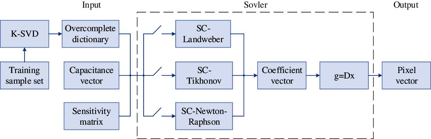
Figure 3: The process of image reconstruction algorithm in ECT
Dictionary learning is the precondition of image reconstruction. It mainly includes the establishment of a training sample set and a learning algorithm. The training sample of this experiment is obtained by simulation in COMSOL5.4 software. The dictionary learning model has attracted much attention in the past few decades, and has been used in fields including image processing, signal restoration and pattern recognition. For the input audio feature, when it is represented by a set of over-complete basis, under the condition of satisfying a certain sparsity or reconstruction error, an approximate representation of the original audio segment can be obtained, that is, Y
We need to minimize the error after restoration and make X as sparse as possible to obtain a more concise representation of the signal and reduce the complexity of the model. Sparse dictionary learning includes two stages: one is the dictionary construction stage; the other is the use of the constructed dictionary to represent the sample stage. As an effective tool for sparse representation of signals, dictionaries provide a more meaningful way to extract the essential features of signal hiding. Therefore, obtaining a suitable dictionary is the key to the success of the sparse representation algorithm. In this experiment, we choose to learn the dictionary method to initialize a 16
The pixel distribution of the imaging area reflects the accuracy of the real situation inside the pipeline. The sampled number of pixels for the image should be determined before constructing the training sample set. Five different shaped objects are placed in the pipeline that reflect different flow patterns, as shown in Fig. 4a. The “circular” path method is used to form a 961 or 1681 pixel image, and the “square” path method is used to form a 561, 1281 or 5097 pixel image.These different pixel distributions respectively restore images, as shown in Figs. 4b–4f.

Figure 4: Image with different number of pixels. (a) A two-phase distribution which contains object A, B, C, D, E with the same permittivity; The best restored image for this two-phase distribution. (b) The image with 961 pixels. (c) The image with 1681 pixels. (d) The image with 561 pixels. (e) The image with 1281 pixels. (f) The image with 5097 pixels
Selection of the image mainly depends on the restoration of the outline of the contact between the two mediums. In the “circular” path method, Objects B and D in the restored image are positive, but Objects A, C, and E are not. The “square” path method works for objects of any shape, but the quality of the image depends on the number of pixels. All objects are deformed in the 561-pixel image, and the restoration quality is poor. The 5097-pixel image better reflects the real situation inside the pipeline, but the high number of pixels leads to a time-consuming program for the K-SVD algorithm. The 1281-pixel distribution was selected to restore image because the degree of image restoration and the running speed of the K-SVD program is between Figs.4d and 4f.
Training samples were created based on the three model examples shown in Fig. 5. Except for the cross-section radius R1 inside the pipe, the parameters were set randomly. In Fig. 5a, c1(x1, y1) and c2(x2, y2) are the center coordinates of two bubbles, with R2 and R3 as their radii. In Fig. 5b, H1 is the height of the arcs medium. In Fig. 5c, R3, R4, and L are the internal radius, external radius, and thickness of the annular medium.

Figure 5: (a) A model for creating samples with two-bubble distribution, similar models can be used for single-bubble distribution, three-bubble distribution, etc. (b) A model for creating samples with stratified distribution. (c) A model for creating samples with annular distribution
Six types of training samples (a central bubble and an eccentric bubble are collectively called a single bubble) were obtained according to the flow pattern. The distribution for single bubbles, two bubbles, three bubbles, and four bubbles each had 1000 images. 850 images showed stratified distribution, and 863 images showed annular distribution. The training sample set consisted of 5,713 binary images of the internal section of the cylindrical pipe, and some training samples are shown in Fig. 6.
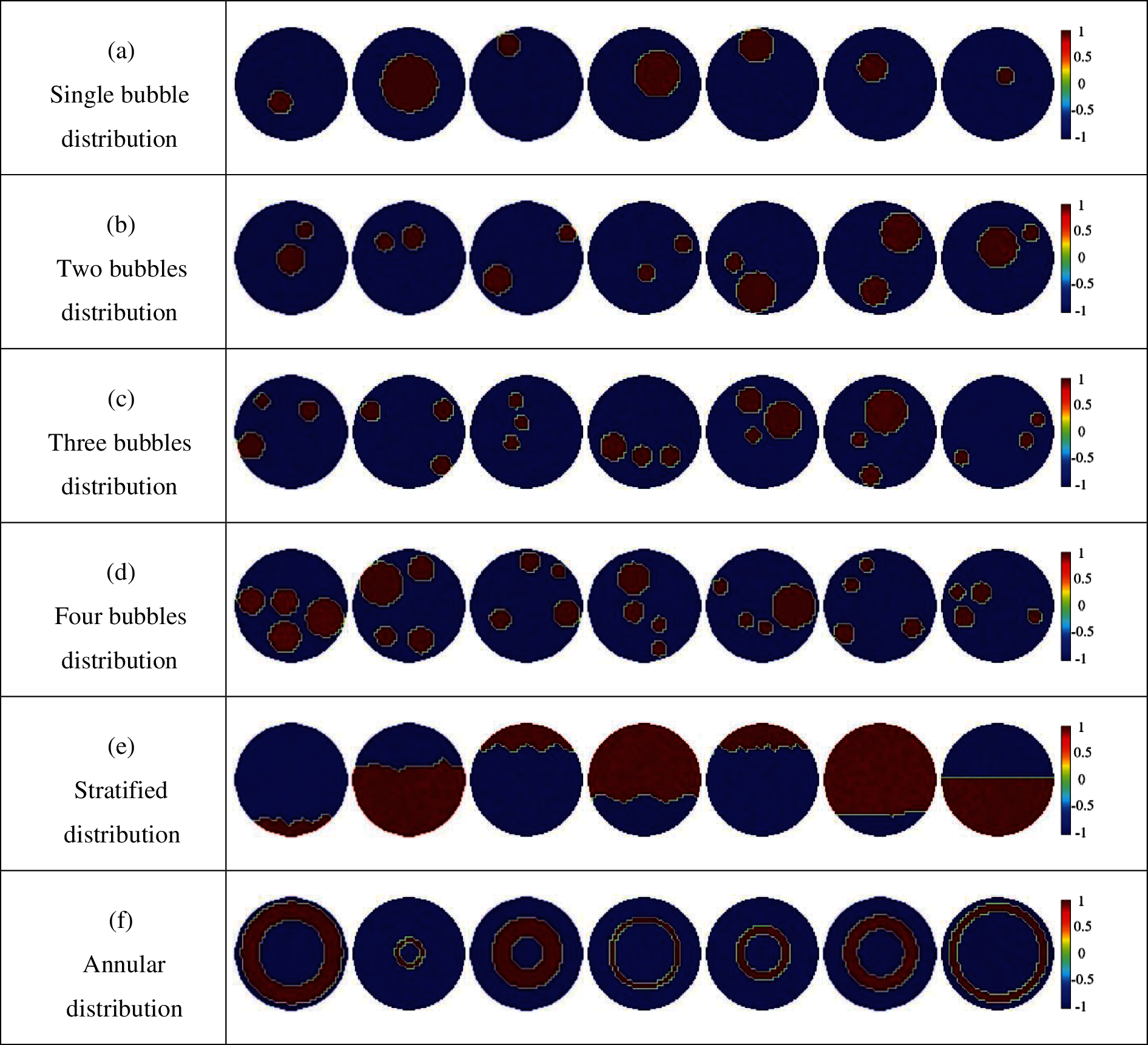
Figure 6: Part of the training sample set
The training samples for the six different distributions were denoted as G1, G2, G3, G4, G5, G6, and the total training sample set was G = [G1, G2, G3, G4, G5, G6]. All samples were randomly sorted and added with slight noise in order to maintain natural conditions and increase the generalization of the overcomplete dictionary. G can be rewritten as
The mathematical model of dictionary learning in D-CS-ECT is as follows:
where
In 2006, Aharon etal. [38] proposed the K-SVD algorithm for dictionary learning. The K-SVD algorithm is a greedy algorithm that realizes signal approximation by alternately optimizing the dictionary and the sparse coefficients. In this paper, the K-SVD algorithm is used to learn the overcomplete dictionary, and its objective function is
where xi is a column vector in X and also the K-sparse sparse coefficient.
There are two stages used by the K-SVD algorithm in training the overcomplete dictionary, which are sparse coding and dictionary updating. In the sparse coding stage, in order to obtain the sparse matrix, the sparse coefficient vector corresponding to each sample is calculated [38–40]. In the dictionary updating stage, atoms in the overcomplete dictionary are updated according to the non-zero elements of the sparse matrix.
The pseudocode for the K-SVD algorithm is as follows:
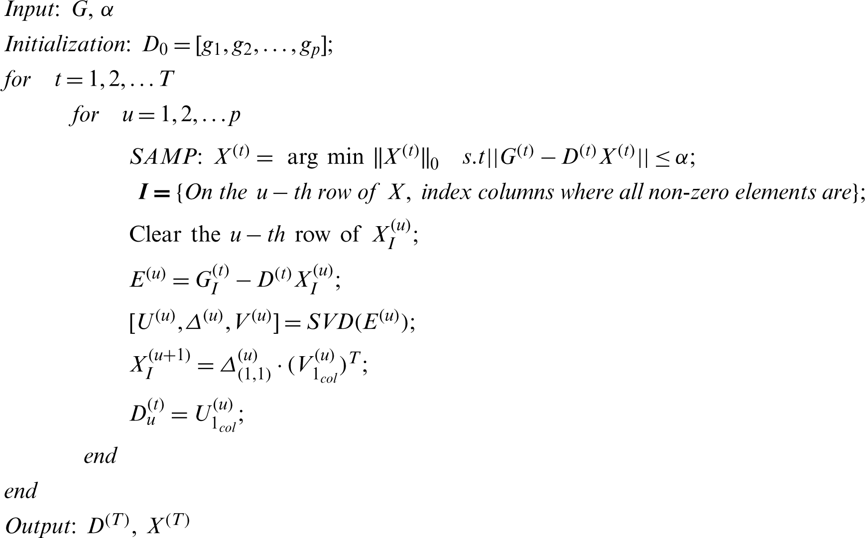
The above pseudocode can be explained by the following four steps:
1. The training dataset
2. The number of atoms in the overcomplete dictionary
3. Sparse coding for G is achieved by using the SAMP algorithm to solve
4. The dictionary is updated column by column after the sparse matrix is obtained. When updating an atom
In this study, the training sample set was large, so the time consumed in the sparse coding stage was much greater than that consumed in the dictionary update stage. Sparse coding was performed by the SAMP algorithm, which is fast in calculating the sparse coefficient vector of a single image and slow in calculating the training sample set. To solve this problem, a parallel computing method was adopted. Considering the computing power and running memory of the computer, the training sample set was evenly divided, and input to the SAMP algorithm was done in batches and in parallel. Sparse coefficient vectors were calculated simultaneously using the CPU and GPU to accelerate the iterations of the K-SVD algorithm.
COMSOL Multiphysics
The measurement target was the two-phase flow in the pipeline, as shown in Fig. 7. R1 and R2 are the radius of the internal cross section and the thickness of the pipeline, respectively, L is the width of the electrode,

Figure 7: Parameters of the pipeline model with COMSOL Multiphysics
The

In order to study the noise resistance of different algorithms, 40 dB of noise was added to the capacitance vector. The imaging results are shown in Fig. 8. For the images reconstructed by the OMP algorithm, almost all distributions show many image artifacts: the bubbles are blurry, and their outlines diverge in multi-bubble distributions. With the GPSR algorithm, the image with the stratified distribution is clear, but target bubbles are deformed in the three-bubble distribution. The central bubble distribution by the NS–Landweber algorithm and the annular distribution by the NS–Tikhonov algorithm are different from their real distribution. Images obtained by the NS–Newton–Raphson algorithm have slight artifacts and slightly deformed bubbles, which enough to reflect the real distribution of the two-phase flow. A reasonable explanation for the poor images is the interference of noise and the soft field, and an incomplete training sample set that cannot cover the majority of the distributions in the two-phase flow.
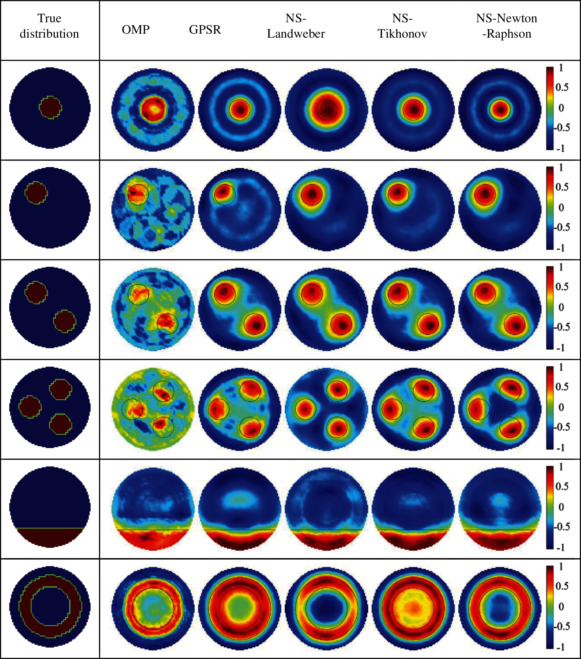
Figure 8: Reconstruction results based on simulation data of noise of SNR = 40 dB
Image error (
where


In order to evaluate the reconstruction quality and stability of the five algorithms more intuitively, the mean and variance of
As shown in Fig. 9, The left picture in Fig. 9 is the average error value. The higher the value, the worse the imaging effect, the lower the value, the better the effect; the right picture is the average correlation coefficient value, the lower the coefficient, the worse the image quality, the higher the coefficient, the higher the image quality. The OMP algorithm has the highest mean for
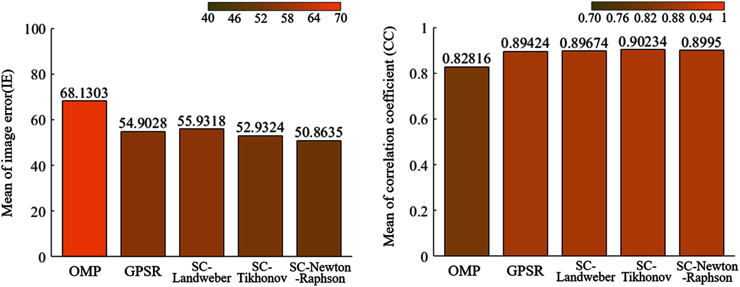
Figure 9: Mean of image error (IE) and correlation coefficient (CC) using different algorithms

Figure 10: Variance of image error (IE) and correlation coefficient (CC) using different algorithms
In this paper, an image reconstruction method based on D-CS-ECT was discussed. Sparse representation of image signal was obtained by training an overcomplete dictionary with K-SVD, and the nonlinear relationship between observation capacitance and the approximate sparse coefficient was solved under the constraint of no sparsity. The two-phase flow in the pipeline was simulated in a noisy environment. Images were reconstructed by the NS–Landweber, NS–Tikhonov, and NS–Newton–Raphson algorithms and compared with the OMP and GPSR algorithms, which are classical sparse constraint algorithms. The NS–Landweber and NS–Tikhonov algorithms were able to reconstruct images clearly on the whole, but unstable reconstructions of the central bubble distribution and annular distribution indicated that the two-phase flow in the central region was not easy to image. The NS–Newton–Raphson algorithm was superior to the other four algorithms in overall image quality and stability, and its highly correlated reconstructed images were closer to the real two-phase flow distribution.
Acknowledgement: I would like to acknowledge Professor, Xuebin Qin, for inspiring my interest in the development of innovative technologies.
Funding Statement: This research was supported by the National Natural Science Foundation of China (No. 51704229), Outstanding Youth Science Fund of Xi’an University of Science and Technology (No. 2018YQ2-01).
Conflicts of Interest: The authors declare that they have no conflicts of interest to report regarding the present study.
1. Sharifi, M., Young, B. (2013). Electrical resistance tomography (ERT) applications to chemical engineering. Chemical Engineering Research & Design, 91(9), 1625–1645. DOI 10.1016/j.cherd.2013.05.026. [Google Scholar] [CrossRef]
2. Cheney, M., Newell, I. (2011). Electrical impedance tomography. Current Opinion in Critical Care, 18(1), 35–41. DOI 10.1109/79.962276. [Google Scholar] [CrossRef]
3. Yu, Z. Z., Peyton, A. T. (1993). Imaging system based on electromagnetic tomography (EMT). Electronics Letters, 29(7), 625–626. DOI 10.1049/el:19930418. [Google Scholar] [CrossRef]
4. Xie, C. G., Plaskowski, A. (1989). 8-electrode capacitance system for two-component flow identification. Part 1: Tomographic flow imaging. IEE Proceedings A (Physical Science Measurement and Instrumentation Management and Education), 136(4), 173–183. DOI 10.1049/ip-a-2.1989.0031. [Google Scholar] [CrossRef]
5. Li, Y., Yang, W., Xie, C. G., Huang, S., Wu, Z. et al. (2011). Gas/oil/water flow measurement by electrical capacitance tomography. Measurement Science & Technology, 24(7), 074001. DOI 10.1088/0957-0233/24/7/074001. [Google Scholar] [CrossRef]
6. Gut, Z., Wolanski, P. (2010). Flame imaging using 3D electrical capacitance tomography. Combustion Science and Technology, 182(10–12), 1580–1585. DOI 10.1080/00102202.2010.497420. [Google Scholar] [CrossRef]
7. Zhang, W., Cheng, Y., Wang, C., Yang, W., Wang, C. H. (2013). Investigation on hydrodynamics of triple-bed combined circulating fluidized bed using electrostatic sensor and electrical capacitance tomography. Industrial & Engineering Chemistry Research, 52(32), 11198–11207. DOI 10.1021/ie4009138. [Google Scholar] [CrossRef]
8. Qiang, G., Meng, S., Wang, D., Zhao, Y., Liu, Z. (2017). Investigation of gas–solid bubbling fluidized beds using ect with a modified tikhonov regularization technique. Aiche Journal, 64(1), 29–41. DOI 10.1002/aic.15879. [Google Scholar] [CrossRef]
9. Zheng, Q., Yang, M., Yang, J., Zhang, Q., Zhang, X. (2018). Improvement of generalization ability of deep cnn via implicit regularization in two-stage training process. IEEE Access, 6, 15844–15869. DOI 10.1109/ACCESS.2018.2810849. [Google Scholar] [CrossRef]
10. Zheng, Q., Tian, X., Jiang, N., Yang, M. (2019). Layer-wise learning based stochastic gradient descent method for the optimization of deep convolutional neural network. Journal of Intelligent and Fuzzy Systems, 37(3), 1–14. DOI 10.3233/JIFS-190861. [Google Scholar] [CrossRef]
11. Jang, J. D., Lee, S. H., Kim, K. Y., Choi, B. Y. (2006). Modified iterative landweber method in electrical capacitance tomography. Measurement Science & Technology, 17(7), 1909. DOI 10.1088/0957-0233/17/7/032. [Google Scholar] [CrossRef]
12. Long, X., Mao, M., Lu, C., Li, R., Jia, F. (2021). Modeling of heterogeneous materials at high strain rates with machine learning algorithms trained by finite element simulations. Journal of Micromechanics and Molecular Physics, 6(1), 2150001. DOI 10.1142/S2424913021500016. [Google Scholar] [CrossRef]
13. Liu, F., Wang, Z., Wang, Z., Qin, Z., Li, Z. et al. (2021). Evaluating yield strength of ni-based superalloys via high throughput experiment and machine learning. Journal of Micromechanics and Molecular Physics, 5(4), 2050015. DOI 10.1142/S2424913020500150. [Google Scholar] [CrossRef]
14. Saxena, S., Animesh, S., Fullwood, M., Mu, Y. (2020). OnionMHC: A deep learning model for peptide–-HLA-A*02:01 binding predictions using both structure and sequence feature sets. DOI 10.21203/rs.3.rs-124695/v1. [Google Scholar] [CrossRef]
15. Chen, Y., Li, H. Y., Xia, Z. J. (2018). Electrical capacitance tomography image reconstruction algorithm based on modified implicit formula landweber method. Computer Engineering, 44(1), 268–273. [Google Scholar]
16. Tian, W., Ramli, M. F., Yang, W., Sun, J. (2017). Investigation of relaxation factor in landweber iterative algorithm for electrical capacitance tomography. IEEE International Conference on Imaging Systems and Techniques. IEEE. DOI 10.1109/IST.2017.8261455. [Google Scholar] [CrossRef]
17. Donoho, D. L. (2006). Compressed sensing. IEEE Transactions on Information Theory, 52(4), 1289–1306. DOI 10.1109/TIT.2006.871582. [Google Scholar] [CrossRef]
18. Lustig, M., Donoho, D., Pauly, J. M. (2007). Sparse mri: The application of compressed sensing for rapid mr imaging. Magnetic Resonance in Medicine, 58(6), 1182–1195. DOI 10.1002/(ISSN)1522-2594. [Google Scholar] [CrossRef]
19. Candès, E. J. (2008). The restricted isometry property and its implications for compressed sensing. Comptes Rendus Mathematique, 346(9–10), 589–592. DOI 10.1016/j.crma.2008.03.014. [Google Scholar] [CrossRef]
20. Jafarpour, S., Molina, R., Katsaggelos, A. K. (2008). Model-based compressive sensing. IEEE International Symposium on Information Theory Proceeding. DOI 10.1109/isit.2011.6034169. [Google Scholar] [CrossRef]
21. Babacan, S. D., Molina, R., Katsaggelos, A. K. (2010). Bayesian compressive sensing using Laplace priors. IEEE Transactions on Image Processing, 19(153–63. DOI 10.1109/TIP.2009.2032894. [Google Scholar] [CrossRef]
22. Wang, H., Fedchenia, I., Shishkin, S., Finn, A., Colket, M. (2012). Electrical capacitance tomography: A compressive sensing approach. IEEE International Conference on Imaging Systems & Techniques. [Google Scholar]
23. Wu, X., Huang, G., Wang, J., Xu, C. (2013). Image reconstruction method of electrical capacitance tomography based on compressed sensing principle. Measurement Science & Technology, 24(7), 75–85. [Google Scholar]
24. Xin. J, W. U., Huang, G. X., Wang, J. W. (2013). Application of compressed sensing to flow pattern identification of ECT. Optics and Precision Engineering. DOI 10.3788/OPE.20132104.1062. [Google Scholar] [CrossRef]
25. Zhang, L. F., Liu, Z. L., Tian, P. (2017). Image reconstruction algorithm for electrical capacitance tomography based on compressed sensing. Tien Tzu Hsueh Pao/Acta Electronica Sinica, 45(2), 353–358. DOI 10.3969/j.issn.0372-2112.2017.02.013. [Google Scholar] [CrossRef]
26. Almurib, H., Kumar, N., Lombardi, F. (2018). Approximate DCT image compression using inexact computing. IEEE Transactions on Computers, 67(2149–159. DOI 10.1109/TC.2017.2731770. [Google Scholar] [CrossRef]
27. Liu, Z., Yin, H., Fang, B., Chai, Y. (2015). A novel fusion scheme for visible and infrared images based on compressive sensing. Optics Communications, 335, 168–177. DOI 10.1016/j.optcom.2014.07.093. [Google Scholar] [CrossRef]
28. You, Z., Raich, R., Fern, X., Kim, J. (2018). Weakly-supervised dictionary learning. IEEE Transactions on Signal Processing, 2527–2541. DOI 10.1109/TSP.2018.2807422. [Google Scholar] [CrossRef]
29. Dou, P., Wu, Y., Shah, S. K., Kakadiaris, I. A. (2018). Monocular 3D facial shape reconstruction from a single 2d image with coupled-dictionary learning and sparse coding. Pattern Recognition, 81, 515–527. DOI 10.1016/j.patcog.2018.03.002. [Google Scholar] [CrossRef]
30. Carrera, D., Boracchi, G., Foi, A., Wohlberg, B. (2018). Sparse overcomplete denoising: Aggregation versus global optimization. IEEE Signal Processing Letters, 24(101468–1472. DOI 10.1109/LSP.2017.2734119. [Google Scholar] [CrossRef]
31. Meribout, M., Saiedmran, M. (2017). Real-time two-dimensional imaging of solid contaminants in gas pipelines using an electrical capacitance tomography system. IEEE Transactions on Industrial Electronics, 64(5), 3989–3996. DOI 10.1109/TIE.2017.2652367. [Google Scholar] [CrossRef]
32. Zhang, L., Yin, W. (2018). Image reconstruction method along electrical field centre lines using a modified mixed normalization model for electrical capacitance tomography. Flow Measurement & Instrumentation, 62, 37–43. DOI 10.1016/j.flowmeasinst.2018.05.011. [Google Scholar] [CrossRef]
33. Guo, Z., Shao, F., Lv, D. (2009). New calculation method of sensitivity distribution for ETC. Yi Qi Yi Biao Xue Bao/Chinese Journal of Scientific Instrument, 30(10), 2023–2026. DOI http://dx.doi.org/10.3321/j.issn:0254-3087.2009.10.003. [Google Scholar] [CrossRef]
34. Candes, E. J., Eldar, Y. C., Needell, D. (2010). Compressed sensing with coherent and redundant dictionaries. Applied and Computational Harmonic Analysis. 31(1), 59–73. DOI 10.1016/j.acha.2010.10.002. [Google Scholar] [CrossRef]
35. Parker, P. A., Bliss, D., Tarokh, V. (2015). CISS 2008. The 42nd Annual Conference on Information Sciences and Systems. IEEE Conference Publication. [Google Scholar]
36. Thong, T. D., Gan, L., Nguyen, N., Tran, T. D. (2010). Sparsity adaptive matching pursuit algorithm for practical compressed sensing. Conference on Signals, Systems & Computers. IEEE. [Google Scholar]
37. Figueiredo, M., Nowak, R. D., Wright, S. J. (2008). Gradient projection for sparse reconstruction: Application to compressed sensing and other inverse problems. IEEE Journal of Selected Topics in Signal Processing, 1(4), 586–597. DOI 10.1109/JSTSP.2007.910281. [Google Scholar] [CrossRef]
38. Aharon, M., Elad, M., Bruckstein, A. (2006). K-SVD: An algorithm for designing overcomplete dictionaries for sparse representation. IEEE Transactions on Signal Processing, 54(11), 4311–4322. DOI 10.1109/TSP.2006.881199. [Google Scholar] [CrossRef]
39. Long, X., Mao, M., Lu, C., Li, R., Jia, F. (2021). Modeling of heterogeneous materials at high strain rates with machine learning algorithms trained by finite element simulations. Journal of Micromechanics and Molecular Physics, 6(1). DOI 10.1142/S2424913021500016. [Google Scholar] [CrossRef]
40. Long, X. Mao, M. H., Lu, C. H., Lu, T. X., Jia, F. R. (2021). Prediction of dynamic compressive performance of concrete-like materials subjected to SHPB based on artificial neural network. Journal of Nanjing University of Aeronautics & Astronautics, 53(5), 789–800. DOI 10.16356/j.1005-2615.2021.05.017. [Google Scholar] [CrossRef]
 | This work is licensed under a Creative Commons Attribution 4.0 International License, which permits unrestricted use, distribution, and reproduction in any medium, provided the original work is properly cited. |