| Computer Modeling in Engineering & Sciences |
DOI: 10.32604/cmes.2022.018338
ARTICLE
Note on a New Construction of Kantorovich Form q-Bernstein Operators Related to Shape Parameter λ
1Fujian Provincial Key Laboratory of Data-Intensive Computing, Key Laboratory of Intelligent Computing and Information Processing, School of Mathematics and Computer Science, Quanzhou Normal University, Quanzhou, 362000, China
2Department of Mathematics, Faculty of Sciences and Arts, Harran University, Şanlıurfa, 63300, Turkey
*Corresponding Author: Reşat Aslan. Email: resat63@hotmail.com
Received: 16 July 2021; Accepted: 23 September 2021
Abstract: The main purpose of this paper is to introduce some approximation properties of a Kantorovich kind q-Bernstein operators related to Bézier basis functions with shape parameter
Keywords: q-calculus; λ-Bernstein polynomials; order of convergence; Lipschitz-type function; Peetre’s K-functional
One of the uncomplicated and most elegant proof of the Weierstrass approximation theorem, the polynomials introduced by Bernstein [1], still guides many studies. Very recently, the quantum calculus shortly (q-calculus), which has numerous applications in various disciplines, has attracted the attention of many authors working on approximation theory. Firstly, Lupaş [2] investigated several approximation properties of the generalizations of q-Bernstein polynomials. Afterward, Phillips [3] obtained some convergence theorems and Voronovskaya type asymptotic formula for the most popular generalizations of the q-Bernstein polynomials. Based on the studies [2,3], many approximation properties of the well-known linear positive operators via q-calculus were investigated in details by several researchers. We refer readers for some notable results [4–13].
In 2007, a Kantorovich type Bernstein polynomials via q-calculus are constructed by Dalmanoğlu [14] as follows:
where
She obtained several approximation properties of the constructed polynomials (1) and estimated the order of approximation in terms of the modulus of continuity. Now, before proceeding further, we recall several basic notations based on q-calculus see details in [15]. Let
The q-factorial [j] q! and q-binomial
and
The q-analogue of the integration on the interval [0, B] is defined as
In 1962’s, French engineer Bézier handled the Bernstein basis functions, since they have a simple construction to utilization, to develop the shape design of surface and curve of cars. Moreover, these magnificent polynomials of Bernstein led to many application fields of Mathematics, such as computer graphics, computer-aided geometric design (CAGD), numerical solution of partial differential equations and, etc. Some applications in CAGD, one can refer to [16 –19].
In 2019, Cai et al. [20] proposed and studied some statistical approximation properties of a new generalization of
where
In the year 2020, Mursaleen et al. [21] considered Chlodowsky kind
Motivated by all write above-mentioned works, we will introduce and examine the following Kantorovich version of
Remark 1.1. Let the operators
For
For
For q = 1, operators (4) reduce to the Kantorovich type
The present research is organized as follows: In Section 2, we compute several preliminary outcomes such as moments and central moments. In Section 3, we give a Korovkin-type convergence theorem and estimate the degree of convergence in terms of the ordinary modulus of continuity, the functions belong to Lipschitz-type class and Peetre’s K-functional, respectively. In the final section, we demonstrate the comparison of the convergence of operators (4) to a function with some illustrations and error estimation table using Maple software.
Lemma 2.1. (See [20]) Let eu(t) = tu,
Lemma 2.2. Let
Proof. Taking into consideration the definition of q-integral, it follows:
Hence, we get (8).
Lemma 2.3 Let
Proof. By simple computing, one has
Then,
In view of (5) and (6), we obtain desired sequel (9).
Lemma 2.4. Let
Proof. As in previous Lemmas, again using the definition of q-integral, we get
By the fact that [j + 1]q = 1+q[j]q, one can has the following easily:
Then, by (5), (6) and (7), we arrive at (10) so the proof is done.
Corollary 2.1. Let
Remark 2.1. It can be seen that for a fixed
3 Convergence Results of R
In this section, we first introduce a Korovkin-type approximation theorem for
Theorem 3.1. Assume that
Proof. Consider the sequence of functions es(y) = ys, where
The proof of (12) follows easily, using (8), (9) and (10). Hence, we get the required sequel.
Now, we will estimate the order of convergence in terms of the usual modulus of continuity, for the function belong to the Lipschitz type class and the Peetre’s K-functional. By first, we symbolize the usual modulus of continuity of
Also, the Peetre’s K-functional is defined by
Taking into account [39], there exists an absolute constant C > 0 such that
Theorem 3.2. Assume that
Proof. Taking
Choosing
Theorem 3.3. Assume that
Proof. Let
Using the Hölder’s inequality and with
Hence, Theorem 3.3 is proved.
Theorem 3.4. For all
Proof. Firstly, we define the following auxiliary operators:
In view of (8) and (9), we find
Using Taylor’s expansion, one has
After operating
Considering (14), we get
On the other hand using (8), (9) and (14), it deduce the following:
With the help of (15) and (16), we get
On account of this, if we take the infimum on the right hand side over all
Hence, we obtain the proof of this theorem.
4 Graphical and Numerical Examples
In this section, we present some graphics and error estimation table to see the convergence behaviour of
Example. Consider the function
on the interval [0, 1].
In Fig. 1, we demonstrate the approximations of
In Fig. 2, we show the approximations of
Also, in Table 1, we calculate the maximum error of approximation of
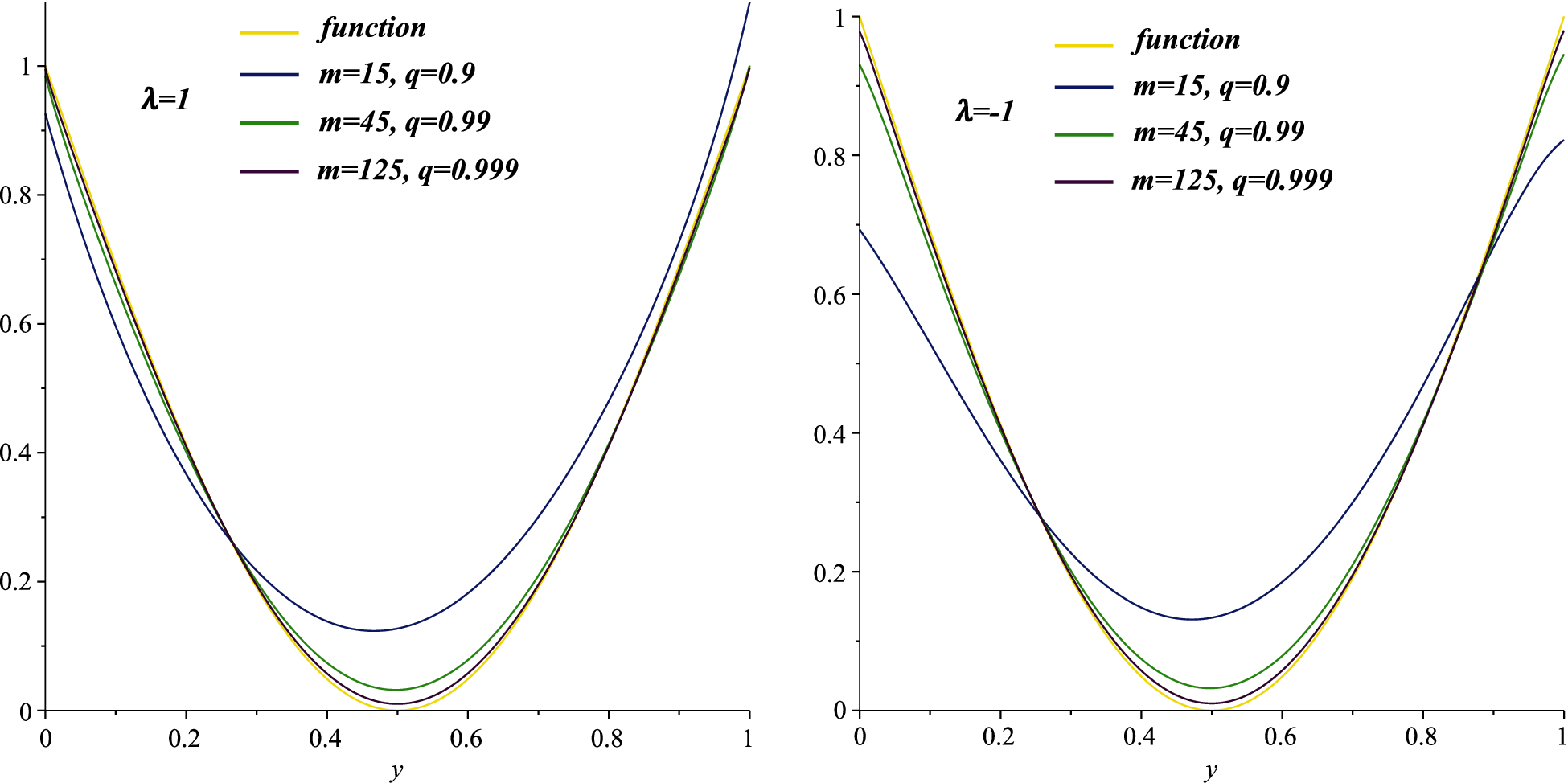
Figure 1: The convergence of
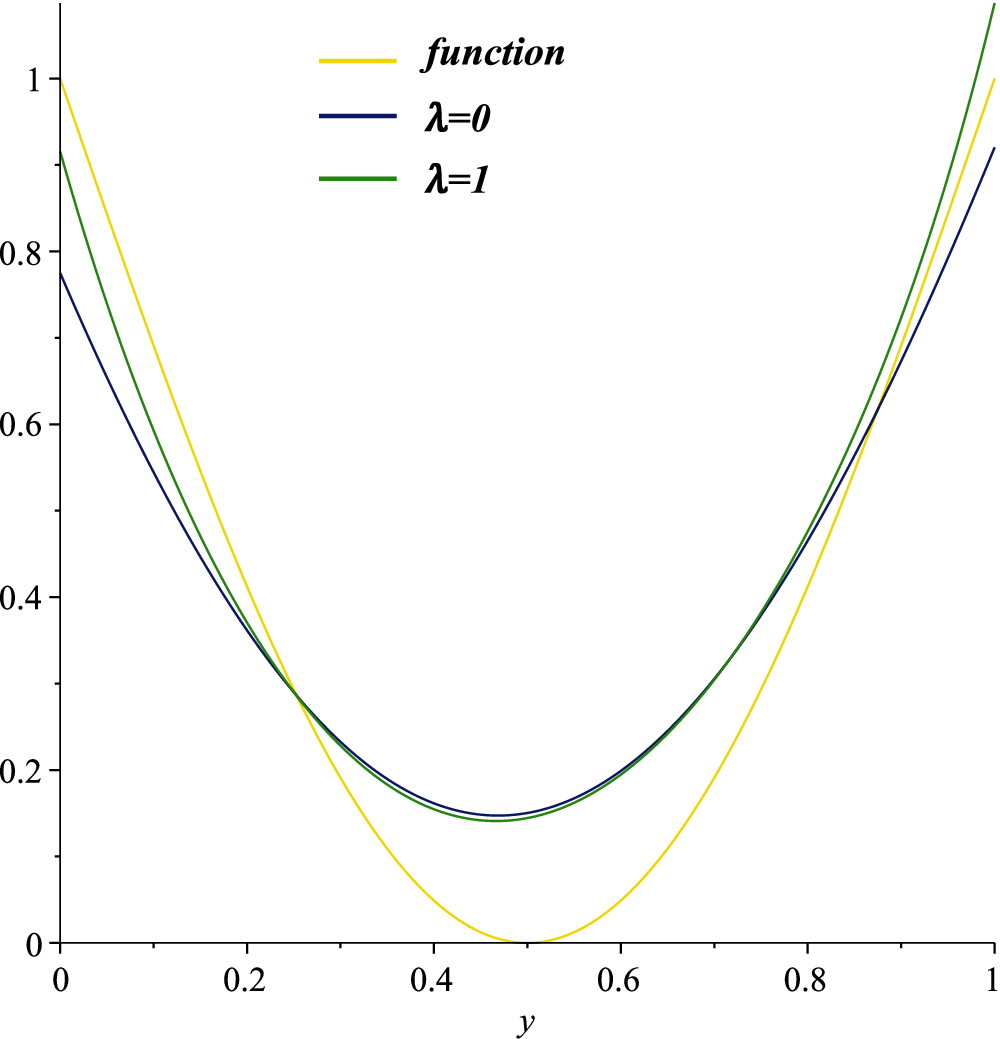
Figure 2: The convergence of
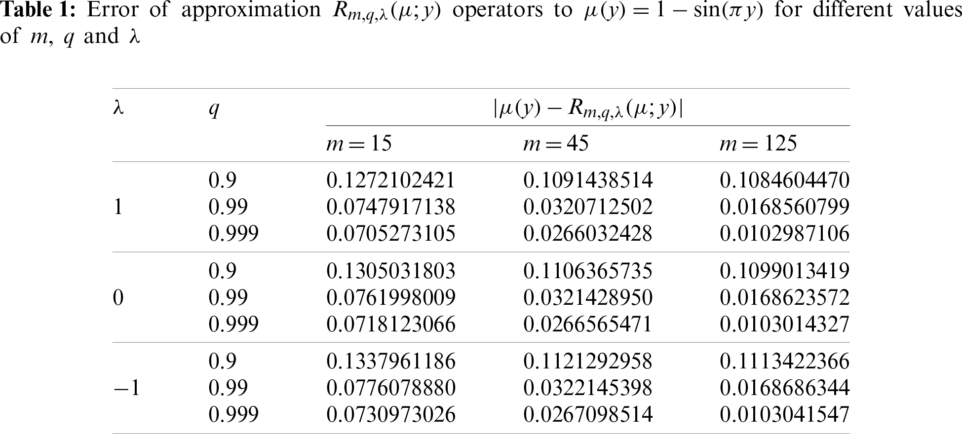
It is obvious from Table 1 that, in case
In this work, we introduced a Kantorovich type of q-Bernstein operators based on the Bézier basis functions with shape parameter
Authors Contributions: The authors contributed equally and significantly in writing this paper. All authors read and approved the final manuscript.
Acknowledgement: We thank Fujian Provincial Big Data Research Institute of Intelligent Manufacturing of China.
Funding Statement: This work is supported by the Natural Science Foundation of Fujian Province of China (Grant No. 2020J01783), the Project for High-Level Talent Innovation and Entrepreneurship of Quanzhou (Grant No. 2018C087R) and the Program for New Century Excellent Talents in Fujian Province University.
Conflicts of Interest: The authors declare that they have no conflicts of interest to report regarding the present study.
1. Bernstein, S. N. (1912). Démonstration du théorème de Weierstrass fondée sur le calcul des probabilités. Communications of the Kharkov Mathematical Society, 13(1), 1–2. [Google Scholar]
2. Lupas, A. (1987). A q-analogue of the Bernstein operator. Seminar on Numerical and Statistical calculus, vol. 9, pp. 85–92. Cluj-Napoca. [Google Scholar]
3. Phillips, G. M. (1997). Bernstein polynomials based on the q-integers. Annals of Numerical Mathematics, 4, 511–518. [Google Scholar]
4. Oruç, H., Phillips, G. M. (2003). q-Bernstein polynomials and Bézier curves. Journal of Computational and Applied Mathematics, 151(1), 1–12. DOI 10.1016/S0377-0427(02)00733-1. [Google Scholar] [CrossRef]
5. Nowak, G. (2009). Approximation properties for generalized q-Bernstein polynomials. Journal of Mathematical Analysis and Applications, 350(1), 50–55. DOI 10.1016/j.jmaa.2008.09.003. [Google Scholar] [CrossRef]
6. Aslan, R., Izgi, A. (2020). Ağırlıklı Uzaylarda q-Szász-Kantorovich-Chlodowsky Operatörlerinin Yaklaşımları. Erciyes Üniversitesi Fen Bilimleri Enstitüsü Fen Bilimleri Dergisi, 36(1), 137–149. [Google Scholar]
7. Mursaleen, M., Khan, A. (2013). Generalized q-Bernstein-Schurer operators and some approximation theorems. Journal of Function Spaces, 2013. DOI 10.1155/2013/719834. [Google Scholar] [CrossRef]
8. Dalmanoğlu, O., Dogru, O. (2010). On statistical approximation properties of Kantorovich type q-Bernstein operators. Mathematical and Computer Modelling, 52, 760–771. DOI 10.1016/j.mcm.2010.05.005. [Google Scholar] [CrossRef]
9. Acar, T., Aral, A. (2015). On pointwise convergence of q-Bernstein operators and their q-derivatives. Numerical Functional Analysis and Optimization, 36, 287–304. DOI 10.1080/01630563.2014.970646. [Google Scholar] [CrossRef]
10. Mahmudov, N. I., Sabancigil, P. (2013). Approximation theorems for q-Bernstein-Kantorovich operators. Filomat, 27, 721–730. DOI 10.2298/FIL1304721M. [Google Scholar] [CrossRef]
11. Neer, T., Agrawal, P. N., Araci, S. (2017). Stancu-Durrmeyer type operators based on q-integers. Applied Mathematics and Information Sciences, 11(3), 1–9. DOI 10.18576/amis/110317. [Google Scholar] [CrossRef]
12. Gupta, V. (2008). Some approximation properties of q-Durrmeyer operators. Applied Mathematics and Computation, 197, 172–178. DOI 10.1016/j.amc.2007.07.056. [Google Scholar] [CrossRef]
13. Karsli, H., Gupta, V. (2008). Some approximation properties of q-Chlodowsky operators. Applied Mathematics and Computation, 195, 220–229. DOI 10.1016/j.amc.2007.04.085. [Google Scholar] [CrossRef]
14. Dalmanoğlu, O. (2007). Approximation by Kantorovich type q-Bernstein operators. Proceedings of the 12th WSEAS International Conference on Applied Mathematics, pp. 113–117. Cairo, Egypt. [Google Scholar]
15. Kac, V., Cheung, P. (2001). Quantum calculus. Berlin, Germany: Springer Science & Business Media. [Google Scholar]
16. Khan, K., Lobiyal, D. K., Kilicman, A. (2018). A de Casteljau Algorithm for Bernstein type Polynomials based on (p, q)-integers. Applications and Applied Mathematics, 13(2), 997–1017. [Google Scholar]
17. Khan, K., Lobiyal, D. K. (2017). Bézier curves based on Lupas (p, q)-analogue of Bernstein functions in CAGD. Journal of Computational and Applied Mathematics, 317, 458–477. DOI 10.1016/j.cam.2016.12.016. [Google Scholar] [CrossRef]
18. Farin, G. (1993). Curves and surfaces for computer-aided geometric design: A practical guide. Amsterdam, Netherlands: Elsevier. [Google Scholar]
19. Sederberg, T. W. (2007). Computer aided geometric design course notes. Provo, Utah: Brigham Young University. [Google Scholar]
20. Cai, Q. B., Zhou, G., Li, J. (2019). Statistical approximation properties of
21. Mursaleen, M., Al-Abied, A. A. H., Salman, M. A. (2020). Chlodowsky type (
22. Rahman, S., Mursaleen, M., Acu, A. M. (2019). Approximation properties of
23. Cai, Q. B., Lian, B. Y., Zhou, G. (2018). Approximation properties of
24. Özger, F. (2019). Weighted statistical approximation properties of univariate and bivariate
25. Özger, F. (2020). On new Bézier bases with Schurer polynomials and corresponding results in approximation theory. Communications Faculty of Sciences University of Ankara Series A1 Mathematics and Statistics, 69, 376–393. DOI 10.31801/cfsuasmas.510382. [Google Scholar] [CrossRef]
26. Özger, F., Demirci, K., Yildiz, S. (2020). Approximation by Kantorovich variant of λ-Schurer operators and related numerical results. In: Topics in contemporary mathematical analysis and applications, pp. 77–94, Boca Raton, USA: CRC Press. [Google Scholar]
27. Özger, F. (2020). Applications of generalized weighted statistical convergence to approximation theorems for functions of one and two variables. Numerical Functional Analysis and Optimization, 41(16), 1990–2006. DOI 10.1080/01630563.2020.1868503. [Google Scholar] [CrossRef]
28. Özger, F., Srivastava, H. M., Mohiuddine, S. A. (2020). Approximation of functions by a new class of generalized Bernstein-Schurer operators. Revista de la Real Academia de Ciencias Exactas, Fsicas y Naturales. Serie A. Matemáticas, 114(4), 1–21. DOI 10.1007/s13398-020-00903-6. [Google Scholar] [CrossRef]
29. Mohiuddine, S. A., Özger, F. (2020). Approximation of functions by Stancu variant of Bernstein-Kantorovich operators based on shape parameter
30. Srivastava, H. M., Ansari, K. J., Özger, F., Ödemiş Özger, Z. (2021). A link between approximation theory and summability methods via four-dimensional infinite matrices. Mathematics, 9(16), 1895. DOI 10.3390/math9161895. [Google Scholar] [CrossRef]
31. Kumar, A. (2020). Approximation properties of generalized
32. Acu, A. M., Manav, N., Sofonea, D. F. (2018). Approximation properties of
33. Cai, Q. B., Torun, G., Dinlemez Kantar, Ü. (2021). Approximation properties of generalized
34. Srivastava, H. M., Özger, F., Mohiuddine, S. A. (2019). Construction of Stancu-type Bernstein operators based on Bézier bases with shape parameter
35. Kantorovich, L. V. (1930). Sur certain dé veloppements suivant les polynômes de la forme de S. Bernstein I, II, pp. 563–568. CR Acad, URSS. [Google Scholar]
36. Cai, Q. B. (2018). The Bézier variant of Kantorovich type
37. Korovkin, P. P. (1953). On convergence of linear positive operators in the space of continuous functions. Doklady Akademii Nauk SSSR, 90, 961–964. [Google Scholar]
38. Altomare, F., Campiti, M. (2011). Korovkin-type approximation theory and its applications. Berlin: de Gruyter. [Google Scholar]
39. DeVore, R. A., Lorentz, G. G. (1993). Constructive approximation. Berlin, Heidelberg: Springer. [Google Scholar]
 | This work is licensed under a Creative Commons Attribution 4.0 International License, which permits unrestricted use, distribution, and reproduction in any medium, provided the original work is properly cited. |