| Computer Modeling in Engineering & Sciences |
DOI: 10.32604/cmes.2022.018134
ARTICLE
Influence of Soil Heterogeneity on the Behavior of Frozen Soil Slope under Freeze-Thaw Cycles
School of Civil Engineering, Hefei University of Technology, Hefei, 230009, China
*Corresponding Author: Yanqiao Wang. Email: wangyanqiao@hfut.edu.cn
Received: 05 July 2021; Accepted: 22 October 2021
Abstract: Soil slope stability in seasonally frozen regions is a challenging problem for geotechnical engineers. The freeze-thaw process of soil slope caused by the temperature fluctuation increases the difficulty in predicting the slope stability because the soil property is influenced by the freeze-thaw cycle. In addition, the frozen soil, which has ice crystal, ice lens and experienced freeze-thaw process, could present stronger heterogeneity. Previous research has not investigated the combined effect of soil heterogeneity and freeze-thaw cycle. This paper studies the influence of soil heterogeneity on the stability of frozen soil slope under freeze-thaw cycles. The local average subdivision (LAS) is utilized to model the soil heterogeneity. A typical slope geometry has been chosen and analysed as an illustrative example and the strength reduction method is used to calculate the factor of safety (FOS) of slope. It has been found that when the temperature is steady, the FOS of the frozen soil slope is influenced by the spatial variability of the thermal conductivity, but the influence is not significant. When the standard deviation and the SOF of the thermal conductivity increase, the mean of the FOS is equal to the FOS of the homogeneous case and the standard deviation of the FOS also increases. After the frozen soil goes through freeze-thaw process, the FOS of the frozen soil slope decreases due to the reduction in the cohesion and the internal friction angle caused by the freeze-thaw cycles. Furthermore, the decreasing ratio of the FOS becomes more scattered after the 5th freeze-thaw cycle compared to that of the FOS after the 1st freeze-thaw cycle. The larger variability of the FOS could induce inaccuracy in the prediction of the frozen soil slope stability.
Keywords: Factor of safety (FOS); freeze-thaw cycle; frozen soil slope; soil heterogeneity; thermal conductivity
In China, the permafrost area is 2.15 × 10⁶ km2, about 22.4% of the country area, and the seasonally frozen soil area is 53.5% of the country area. In the seasonally frozen soil area, slope stability is a challenging problem for geotechnical engineers. The temperature boundary condition, which fluctuates during season changing, poses a serious threat to the stability of the slopes in this region [1,2]. The fluctuation of temperature induces the freezing and thawing processes of frozen soil. There are many reported slope failures caused by the freezing and thawing processes [3]. Unlike the slope failure in the permafrost region, where the temperature is constantly below 0°C for at least two consecutive years [4,5], the freeze-thaw cycle in the seasonally frozen region is considered as an important factor for the slope failure.
In the frozen soil regions, the freezing and thawing processes change the internal structures of soil skeleton and the connection between soil particles, and further change the soil properties. Since 1980s, the study of the influence of freeze-thaw cycle on the soil properties has been undertaken by researchers and engineers. For the thermal parameters of soils, the research on the influence of freeze-thaw cycle is limited. In those researches, Moghbel et al. [6] has done some investigations on the biocover made of compost. They found that the freeze-thaw cycles influence the thermal conductivity of compost biocover. In addition, the thermal conductivity approximately reduced to 80% of its original value, and the reduction mainly occurs in the first three freeze-thaw cycles. Cheng et al. [7] have studied the influencing factors of the thermal conductivity of the silty soil. It was found that the thermal conductivity decreases after the freeze-thaw process. In their tests, the number of freeze-thaw cycles is 3. After the third cycle, the deduction of the thermal conductivity is from 20% to 40% of the original value for different water contents and dry densities. Xiao [8] found the thermal conductivity of clay in Shanghai reduces after the freeze-thaw cycle. From the above limited researches, the thermal conductivity of soil generally reduces after the freeze-thaw cycle. The reduction usually occurs in the first few cycles, and the extent of reduction is also influenced by other soil properties, such as water content and dry density.
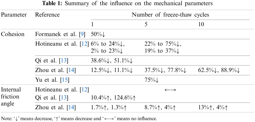
As to the mechanical parameters, the investigation of the influence of freeze-thaw cycle has started early in the 1980s. Formanek et al. [9] found the first freeze-thaw cycle results in a 50% reduction of the cohesion of the silt loam. In the following two cycles, the cohesion almost remains stable. Graham et al. [10] pointed out that the strength of clay at low stresses decreases due to the freeze-thaw cycle. Ma et al. [11] investigated the influence of freeze-thaw cycle on the strength of silt stabilized with lime. Through the tests, it was found that the influence of freeze-thaw cycle on the lime silt is more significant than that on the silt. In addition, the strength of the lime silt decreases after the freeze-thaw cycle and the reduction could be 35% after 10 cycles. Hotineanu et al. [12] investigated the impact of freeze-thaw cycle on the mechanical properties of two types of clayey soils (high plasticity-bentonite and low plasticity-kaolinite), stabilized with lime. The test results show the freeze-thaw cycle mainly affects the cohesion, whereas the impact on the internal friction angle is not obvious. For the bentonite, the reduction of cohesion after the first cycle is from 6% to 24% of the original value for soils without stabilization and soils stabilized with lime and cured with different time durations. After the fifth cycle, the reduction is from 22% to 75% of the original value. For the kaolinite, the reduction is less than that of the bentonite. After the first cycle, the reduction is from 2% to 23% of the original value. After the fifth cycle, the reduction is from 19% to 37% of the original value. Qi et al. [13] studied two over-consolidated soils, i.e., silty clay and loess. They found the cohesion of the two soils decrease after 1 cycle, but the internal friction angle increases. The reduction of cohesion is 38.6% for loess and 51.1% for silty clay. The increase of internal friction angle is 10.4% for loess and 124.6% for silty clay. Zhou et al. [14] also conducted tests on the undisturbed and saturated samples of loess. Their results showed that the cohesion decreases with the number of freeze-thaw cycles, while the internal friction angle increases for both the undisturbed and saturated samples. For the undisturbed and saturated samples, the variation of cohesion and internal friction angle occurs mainly in the early 10 cycles. After 10 cycles, the decrease of cohesion is up to 62.5% for the undisturbed samples and 88.9% for the saturated samples. Meanwhile, the increase of the internal friction angle is up to 13% for the undisturbed samples and 4% for the saturated samples. The influence on the internal friction angle is insignificant. Yu et al. [15] conducted tests on the saturated silty clay. They found that after 5 cycles, the changes of the cohesion and internal friction angle gradually become stable. In the previous 5 cycles, the cohesion decreases and the internal friction angle increases. The reduction of the cohesion is up to 75% of the original value. Table 1 has concluded the findings from the previous researches. In general, the cohesion increases due to the freezing-thawing process, whereas the internal friction angle could increase or remain stable.
In addition to the influence of freeze-thaw cycle, the property of frozen soil exhibits significant spatial variability. Normal natural soils have been recognized as heterogeneous materials [16]. Frozen soil, which has ice crystal, ice lens and experienced freeze-thaw process, could present stronger heterogeneity. The heterogeneity definitely affects the slope stability in the seasonally frozen area. Alonso [17] has pointed out that the slope could fail even when the computed single factor of safety (FOS) without considering the soil heterogeneity was larger than 1.0. For the normal slopes, the influence of soil heterogeneity in the strength parameters (i.e., cohesion and friction angle) and the hydraulic parameters (e.g., the saturated hydraulic conductivity) on the slope stability has been considered since 1970s, such as Wu et al. [18], Cornell [19], Tang et al. [20], Vanmarcke [21], Gui et al. [22], Griffiths et al. [23], Liu et al. [24,25], etc. Many methods have been developed to analyse the slope stability from a probabilistic perspective. The commonly used methods include the first order second moment (FOSM), first order reliability method, point estimate method and Monte Carlo method (MCM). Among them, although the MCM is time consuming, with the development of computer science, this disadvantage can be overcome. The MCM has the advantage of being more accurate in the probabilistic analysis of slope stability.
For the frozen soil slope, the research concerning the influence of soil heterogeneity on the frozen soil slope stability is seldom. Xu et al. [26] and Zhang [27] analysed an infinite frozen soil slope by using the limit equilibrium method and the MCM. In their research, the cohesion and friction are assumed to be uniformly distributed. Li et al. [28] and Guo et al. [29] analysed an infinite frozen soil slope by using the limit equilibrium method and the FOSM. In addition to the cohesion and friction angle, the unit weight of frozen soil, the frost heaving amount and the snow depth are all considered to be heterogeneous. Chen et al. [30] combined the MCM with random field to investigate the slope stability in permafrost area. The Karhunen-Loève expansion was used to generate the random field of hydraulic and thermal conduction.
Therefore, from the previous research, it has been found that it is worth investigating the frozen soil slope stability under the combined effect of soil heterogeneity and the freeze-thaw cycle. In this paper, firstly, the equations used to determine the temperature and pore water pressure are introduced. Then, the strength reduction method for the slope stability analysis is presented. After that, the random field generator, i.e., the local average subdivision (LAS), has been introduced. Later, an illustrative example is analysed to investigate the combined effect of soil heterogeneity and the freeze-thaw cycle.
2 Governing Equations Used in the Calculation of Frozen Slope Stability
2.1 Equations for Heat Transportation and Pore Water Pressure
In this paper, since the heat transfer in soils occurs mainly by conduction, the heat convection is not considered [31,32]. Thus, the two-dimensional heat transport equation for a freezing soil can be written as follows [33–35] with the coupling behavior between heat and moisture migration being neglected:
where, T is the temperature, λx and λy are the thermal conductivity in the x and y direction, respectively, which is assumed to be the same in this paper. C is the volumetric heat capacity of soil, t is time. For a steady state boundary condition, i.e., the temperature is constant, the above equation can be simplified as:
The above equation is solved by the finite element method. After the temperature is computed out, then the pore water pressure can be calculated based on the following relationship when the temperature is below zero [36,37]:
in which, a and b are the constant parameters which are related to the physical properties of soil and can be determined by experiments. θu is the unfrozen volumetric water content. By using the following van Genuchten-Mualem equation [38], the negative pore water pressure head h can be calculated from θu by using the following equation:
where, θs and θr are the saturated and residual volumetric water content, respectively. α is a parameter which is approximately the inverse of the air-entry suction head. n and m are the fitting parameters of the soil water retention curve, and m = 1–1/n [39]. After the negative pore water pressure is computed out, the results can be exported to the slope stability computation.
2.2 Equations for Slope Stability
The previous results of pore water pressure can be imported to generate the effective stress field first. Bishop's effective stress combined with the extended Mohr-Coulomb failure criterion is used here to model the shear strength, soils are considered to be an elastic, perfectly-plastic material:
in which, c′ and ϕ′ are the effective cohesion and internal friction angle. σ is the total stress generated by the gravitational load and s is suction, which is equal to:
where, ua is the pore air pressure, which is assumed to be atmospheric in this paper, uw is pore water pressure. χ is a scalar parameter defining the suction induced effective stress, χ is defined as follows:
Then, the FOS of the slope is computed using the strength reduction method, that is:
where, cf′ and ϕf′ are the factored effective cohesion and internal friction angle corresponding to the slope failure.
2.3 Random Field Modelling of Soil Parameter
Soil parameters are inherently heterogeneous. The values of soil parameters in the field are spatially variable. In order to model the spatial variability, random field theory has been developed. The LAS, which is a commonly used method to generate random field, is applied in this paper. Fenton [40] compared several methods of generating random field, such as the turning bands method, the fast Fourier transform and the LAS. The LAS was shown to be more efficient and reliable. Moreover, it is ideally suited for use with the finite element method (FEM).
The LAS is a recursive division process. Initially, a square domain is assigned with an initial value which is computed using a standard normal distribution and a correlation function. Then the domain is divided into four random cells. Among them, the values of three cells are computed by the LAS, and the other one is calculated by the upward averaging. After that, the division process is continued until the number of random cells achieves the requirement (related to the number of finite elements). Finally, the standard random fields can be transformed to the required fields which follow the input distribution. The generated random field is isotropic and can be postprocessed to give an anisotropic random field if different values of scales of fluctuation are used in the horizontal and vertical directions.
An exponential Markov correlation function is taken as follows:
where, ρ(τv, τh) is the correlation coefficient between the values of two points, τv and τh are the lag distance between two points in the vertical and horizontal directions in a random field, respectively. θv and θh are the vertical and horizontal scales of fluctuation, respectively. The reader is referred to Samy [41] and Spencer [42] for the detailed implementation of the LAS.
2.4 Framework of the Overall Analysis
Fig. 1 shows the flowchart of the probabilistic analysis of the heterogeneous frozen slope by considering the spatial variability of the thermal conductivity. The detailed procedures are summarized as follows:
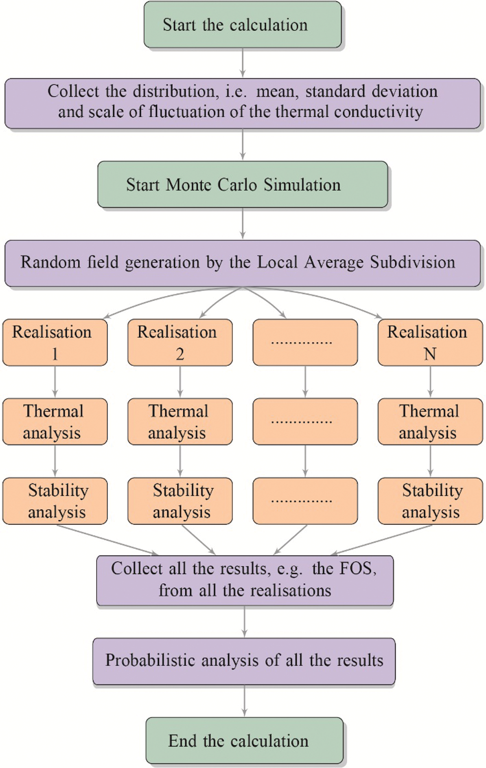
Figure 1: Flowchart of the overall analysis
• Collect the necessary information for soil parameters, i.e., the thermal conductivity in this paper, which will be used in the following random field generation, such as the mean, the standard deviation, and the scale of fluctuation.
• Generate a random field of the thermal conductivity using the LAS. Multiple realizations of the random field are generated.
• Map the value of random cells in each realization to each Gauss point in the finite elements. Then, the thermal analysis is conducted to solve the temperature distribution of each realization. Then, the unfrozen volumetric water content and the pore water pressure is worked out.
• Import the computed results of the unfrozen volumetric water content and the pore water pressure of each realization to the stability calculation of the slope.
• Collect all the computed results of the FOS from all the realizations and carry out the probabilistic analysis.
In this paper, in order to investigate the influence of soil heterogeneity on the behavior of frozen soil slope, a typical slope geometry presented in the Program 6.4 of Smith et al. [43] is utilized, seen in Fig. 2. The slope is 10 m high with a slope ratio 1:2, and the crest is 20 m wide. The foundation is 60 m wide and 5 m deep.
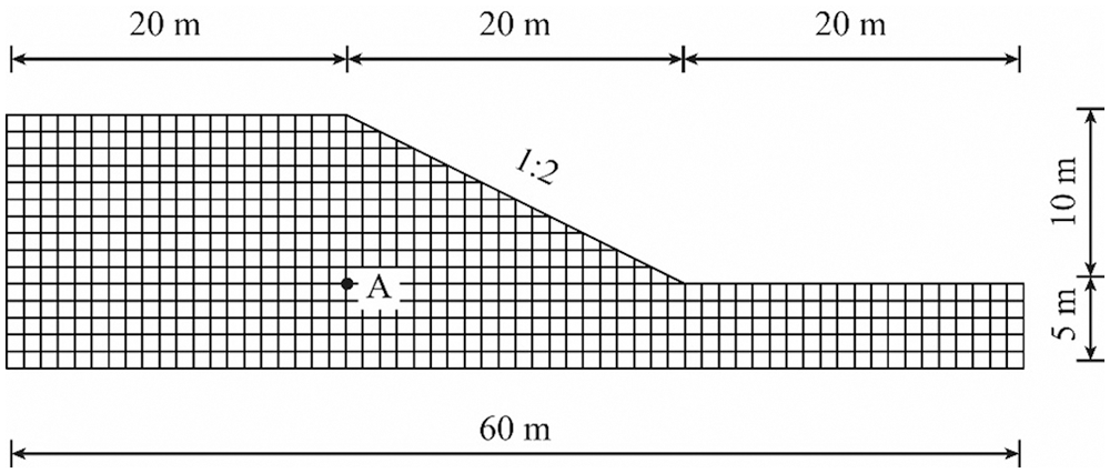
Figure 2: Geometry of the analysed slope
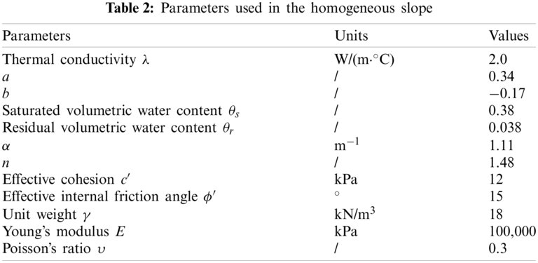
For comparison, the thermal, hydraulic and mechanical parameters are all first considered to be homogeneous across the whole domain. The values of those parameters are listed in Table 2. The boundary conditions are: the temperature of the bottom is −5°C and the temperature of the top surface is −20°C [44,45].
In the finite element analysis, the whole domain is discretised and the size of element is 1.0 m by 1.0 m (see Fig. 2). When the parameters are all considered to be uniform across the whole domain, the computed distribution of the temperature and the pore water pressure is shown in the following Fig. 3.
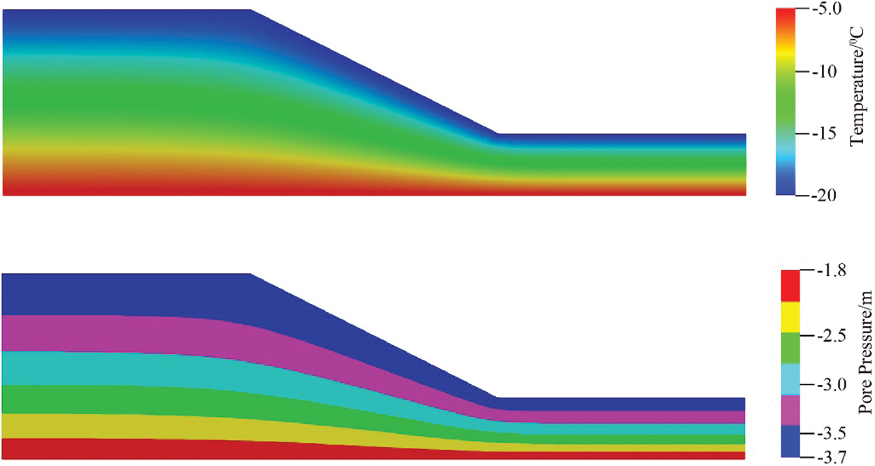
Figure 3: Distribution of temperature and pore pressure head in the slope
Since the pore water pressure has been computed out, the results can be imported to the slope stability calculation. Fig. 4 gives the results of the strength reduction factor, the maximum nodal displacement at convergence and the number of iterations to achieve convergence. Since the iteration ceiling is chosen to be 500, the computed FOS is 1.446.
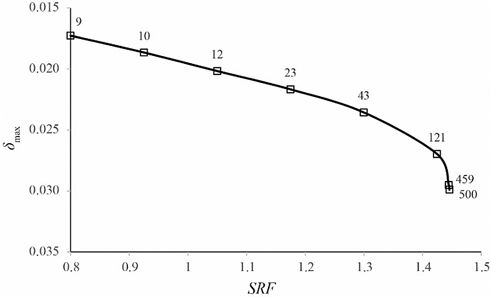
Figure 4: Maximum nodal displacement vs. strength reduction factor (SRF)
In the Introduction section, it has been found that the freeze-thaw cycle affects the mechanical parameters, i.e., the cohesion and the internal friction angle. From Table 1, it is assumed that, after the first freeze-thaw cycle, the effective cohesion decreases from 12 to 10 kPa and the effective internal friction angle increases from 15o to 16o. The computed FOS of the slope is 1.424. It can be seen that the FOS decreases due to the impact of the freeze-thaw cycle on the mechanical parameters. The decreasing ratio is small, i.e., 1.52%.
Since the frozen soil has strong heterogeneity, the thermal conductivity is taken to be a spatially variable here. First, the influence of the heterogeneity in the thermal conductivity on the temperature and pore pressure distribution is investigated. Currently, there are seldom researches investigating the heterogeneity of the thermal conductivity. Usowicz et al. [46] studied a cultivated field with 220 measuring points. In the fields, the water content and bulk density of the topsoil were measured. Then, the thermal conductivity of the soil was estimated based on a statistical-physical model. From the calculated thermal conductivity, the classical statistics and geostatistics were used to analyse the variation and spatial correlation of the thermal conductivity. It was found that the distribution of the thermal conductivity is normal, and the spatial correlation function is spherical or exponential. Ferguson [47] investigated the effect of heterogeneity in the thermal conductivity on heat transport in aquifers. The thermal conductivity was assumed to be normally distributed. Due to a lack of geostatistical information, there was no spatial correlation considered in the thermal conductivity. Simms et al. [48] examined the impact of heterogeneity in the thermal conductivity on the functioning of horizontal ground heat exchangers. They took use of previous studies on soil hydraulic properties and assumed that the spatial correlation of the thermal conductivity is the same as that of the soil hydraulic properties. In this paper, in order to examine the variation of the temperature field and pore pressure distribution under the impact of the heterogeneous thermal conductivity, different statistics (see Table 3) of the thermal conductivity was used.
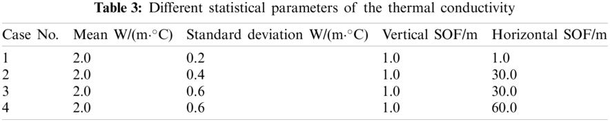
Table 3 shows the different statistical parameters of the thermal conductivity. Based on the different parameters, the random fields of the four cases generated by the LAS show significant difference (seen in Fig. 5). From Fig. 5, it can be seen that the slope becomes layering with the increase of the horizontal SOF. In addition, by comparing Figs. 5b and 5c, it can be found that the color of Fig. 5c is darker. It means when the standard deviation of the thermal conductivity increases, the range of the values of the thermal conductivity increases.
In order to investigate the influence of the heterogeneity in the thermal conductivity on the temperature and pore water pressure distributions, a point A in the slope (shown in Fig. 2) is chosen to show the variation of the values. Fig. 6 shows the probability density function (PDF) and cumulative distribution function (CDF) of the temperature of point A from 500 realisations of the random field under different statistical parameters of the thermal conductivity. The mean and standard deviation of the temperature are summarized in the following Table 4.
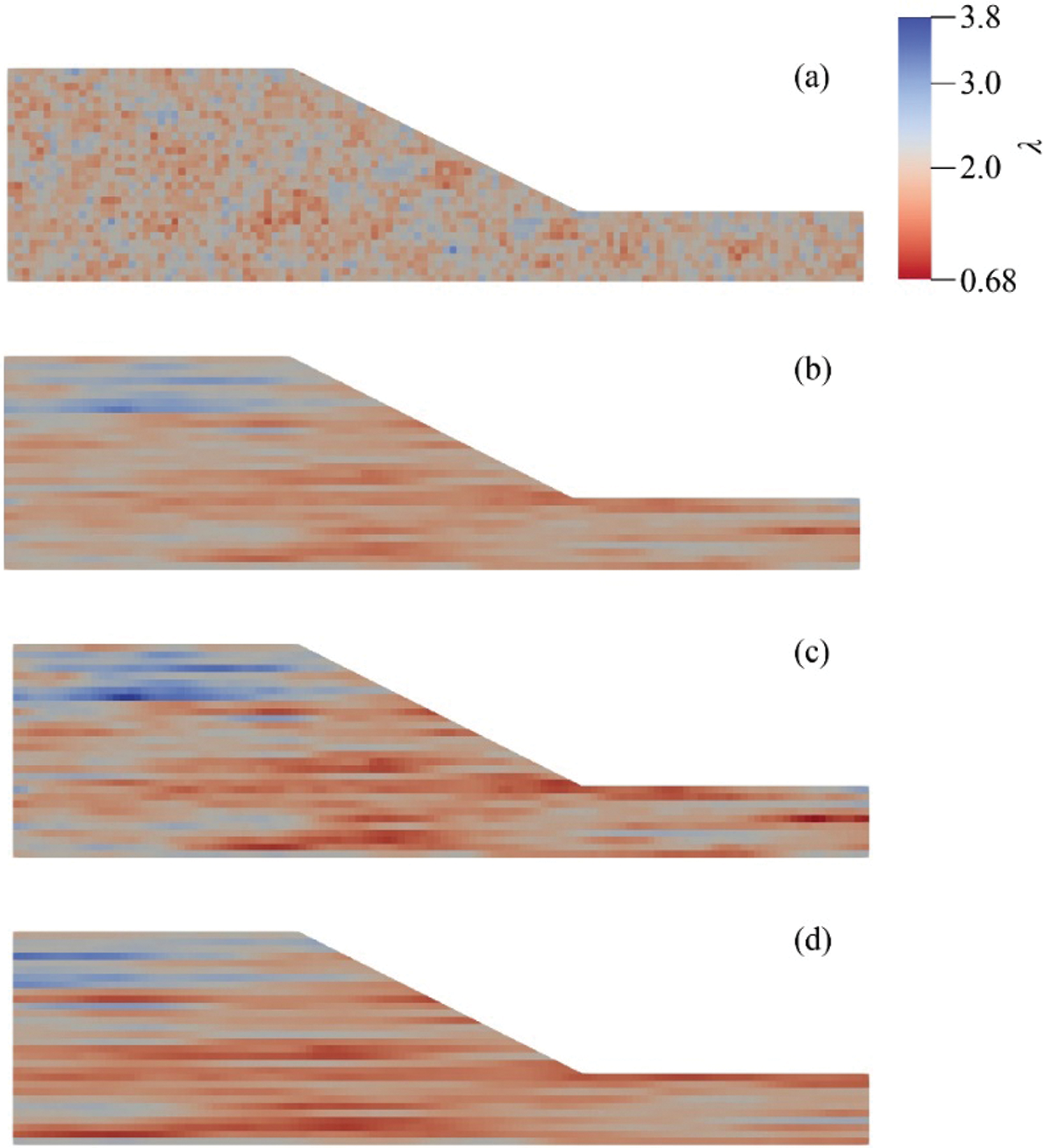
Figure 5: Realisations of the random field with different statistical parameters: (a) Case 1; (b) Case 2; (c) Case 3 and (d) Case 4
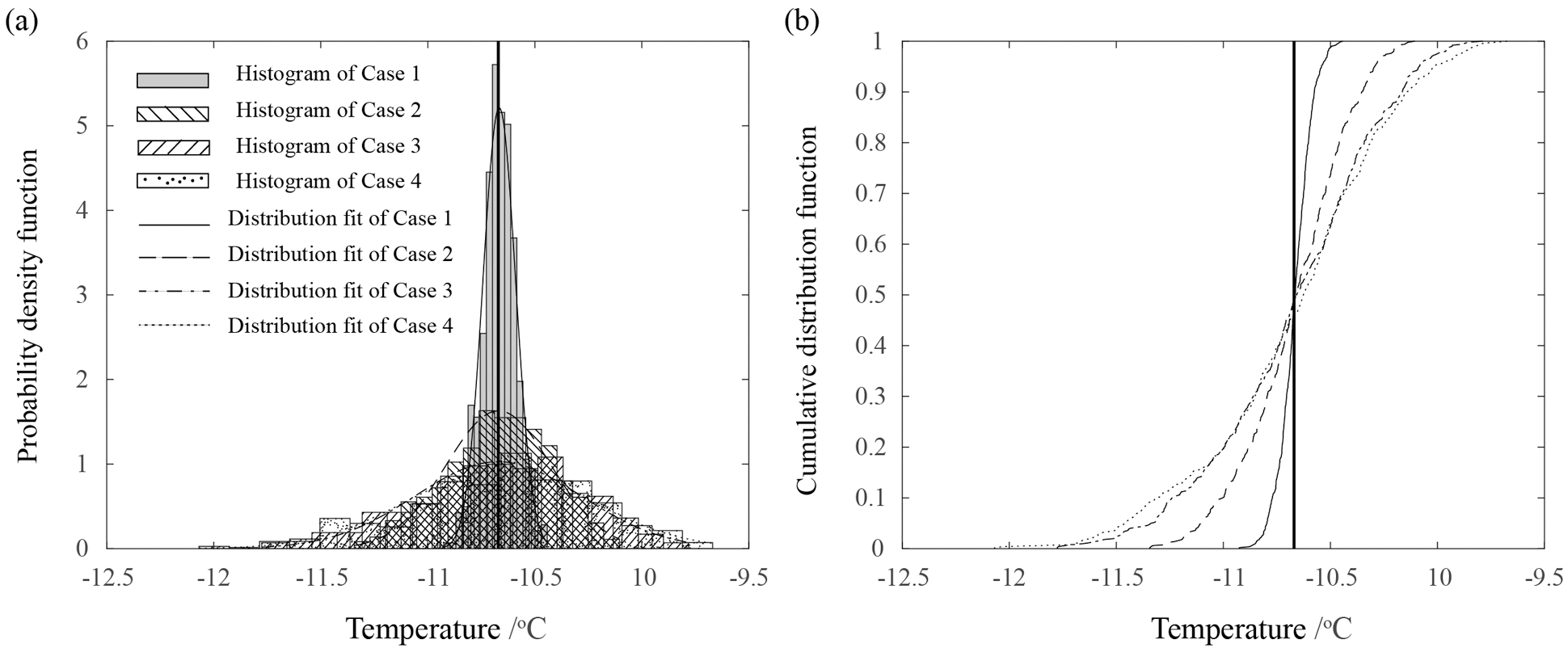
Figure 6: PDFs (a) and CDFs (b) of the temperature of point A under different statistical parameters of the thermal conductivity
From Fig. 6, the distribution of the temperature is normal. In Table 4, the mean of the temperature of point A in the heterogeneous slope is equal to the result of the homogeneous slope. Generally, it can be found that the variation of the temperature, i.e., the standard deviation of the temperature, of point A increases with the increase of the standard deviation or the horizontal SOF of the thermal conductivity.
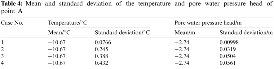
Based on Eqs. (3) and (4), the results of the corresponding pore water pressure in the slope can be acquired. Fig. 7 shows the results of the pore water pressure head of point A from 500 realisations. Due to the relationship between the temperature and the pore water pressure, the variation of the pore water pressure head is similar to that of the temperature under different statistics of the thermal conductivity.
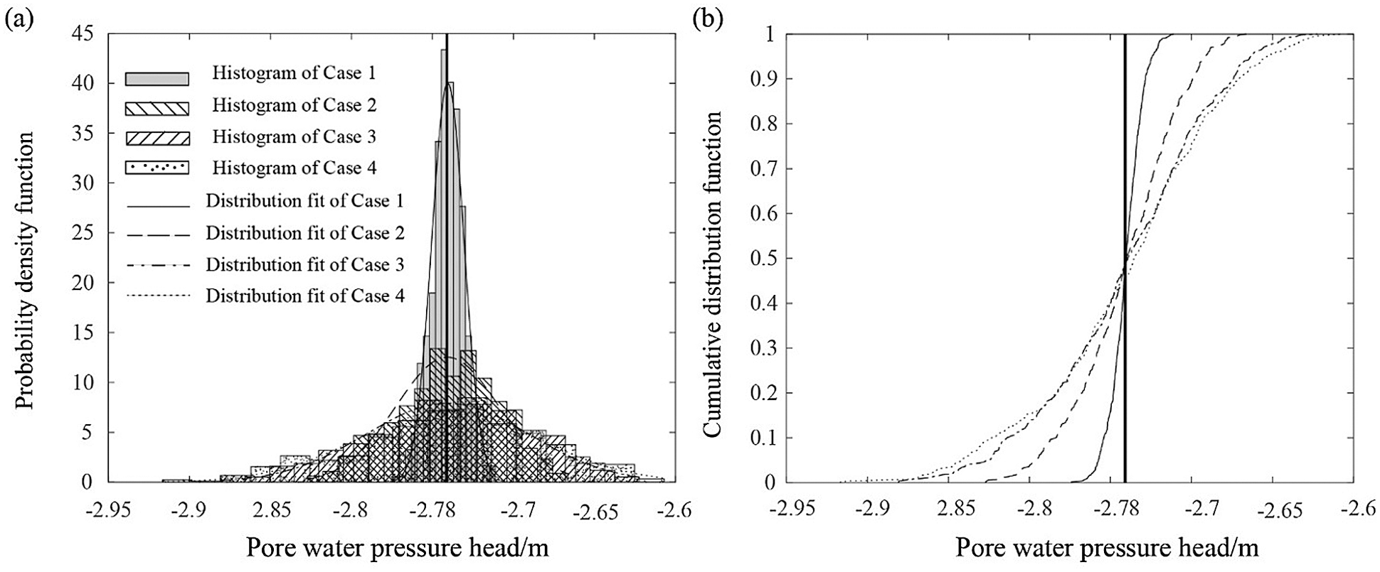
Figure 7: PDFs and CDFs of the pore water pressure head of point A under different statistical parameters of the thermal conductivity
Then, the results will be imported into the slope stability analysis. The FOS of 500 realisations of each case can be computed out. Fig. 8 shows the histogram of the FOS for each case. In Fig. 8, the horizontal axis denotes the FOS, and the vertical axis represents the number of realisations with a certain FOS. Generally, when the standard deviation or the horizontal SOF increases, the results of FOS become scatter. Moreover, from Figs. 8b–8d, the distribution of the FOS is approximately normal. This proves that the heterogeneity of the thermal conductivity indeed affects the frozen slope stability. However, it can be seen that the influence of the thermal conductivity on the FOS of the frozen slope is limited. The values of the FOS vary in a small scale.
Figure 8: Histogram of the FOS of the slope under different statistical parameters of the thermal conductivity: (a) Case 1; (b) Case 2; (c) Case 3 and (d) Case 4
In order to further investigate the influence of freeze-thaw cycle on the heterogeneous frozen slope stability, similar to the homogeneous case, the effective cohesion decreases from 12 to 10 kPa and the effective internal friction angle increases from 15° to 16° after the first freeze-thaw cycle. In order to investigate the influence of freeze-thaw cycle on the stochastic analysis of the slope stability, the decreasing ratio of the FOS caused by the freeze-thaw cycle has been defined here:
in which, r is the decreasing ratio,
Fig. 9 shows the variation of the decreasing ratio r for all the realisations of the four cases. The horizontal axis is the number of realisation. From Fig. 9, it can be seen that the FOS decreases after the first freeze-thaw cycle due to the reduction in the strength parameters, i.e., the effective cohesion and the effective internal friction angle. The decreasing ratios r are generally around 1.52%, which is equal to the result of the homogeneous slope. Moreover, when the standard deviation and the horizontal SOF increase, the decreasing ratio r presents more variability. The reason is that the variation of the FOS increases (shown in Fig. 8) when the standard deviation and the horizontal SOF increase.
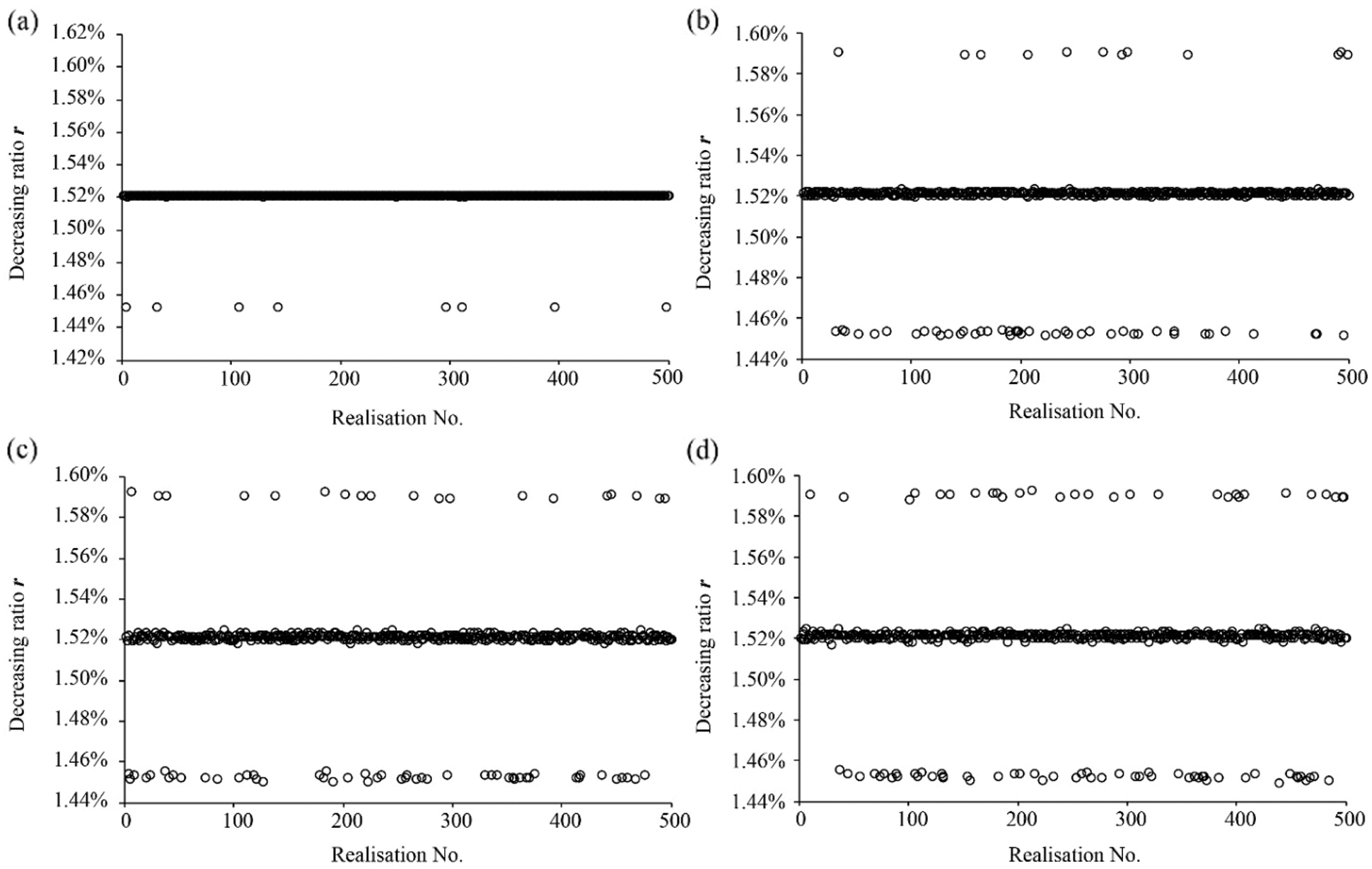
Figure 9: Decreasing ratios of the FOS for the four cases after the 1st freeze-thaw cycle: (a) Case 1; (b) Case 2; (c) Case 3 and (d) Case 4
Furthermore, after 5th freeze-thaw cycle, it is assumed based on Table 1 that the effective cohesion reduces to 6 kPa and the effective friction angle remains 16°. Fig. 10 shows the variation of the decreasing ratio r for all the realisations of the four cases. The FOS decreases more due to the reduction of the effective cohesion. The decreasing ratios r are around 14%. Meanwhile, compared to Fig. 9, it can be seen that the dispersion of the FOS becomes more obvious. The reason of the dispersion could be that, with the number of freeze-thaw cycle increasing, the cohesion decreases more after 5th freeze-thaw cycles. From Eq. (5), the influence of the suction becomes more dominant after the decrease of the cohesion. Therefore, the influence of the variability in suction caused by the heterogeneity of the thermal conductivity on the FOS becomes more significant. The stronger dispersion means that the estimation of the stability of the frozen soil slope by considering the thermal conductivity as homogeneous could be inaccurate.
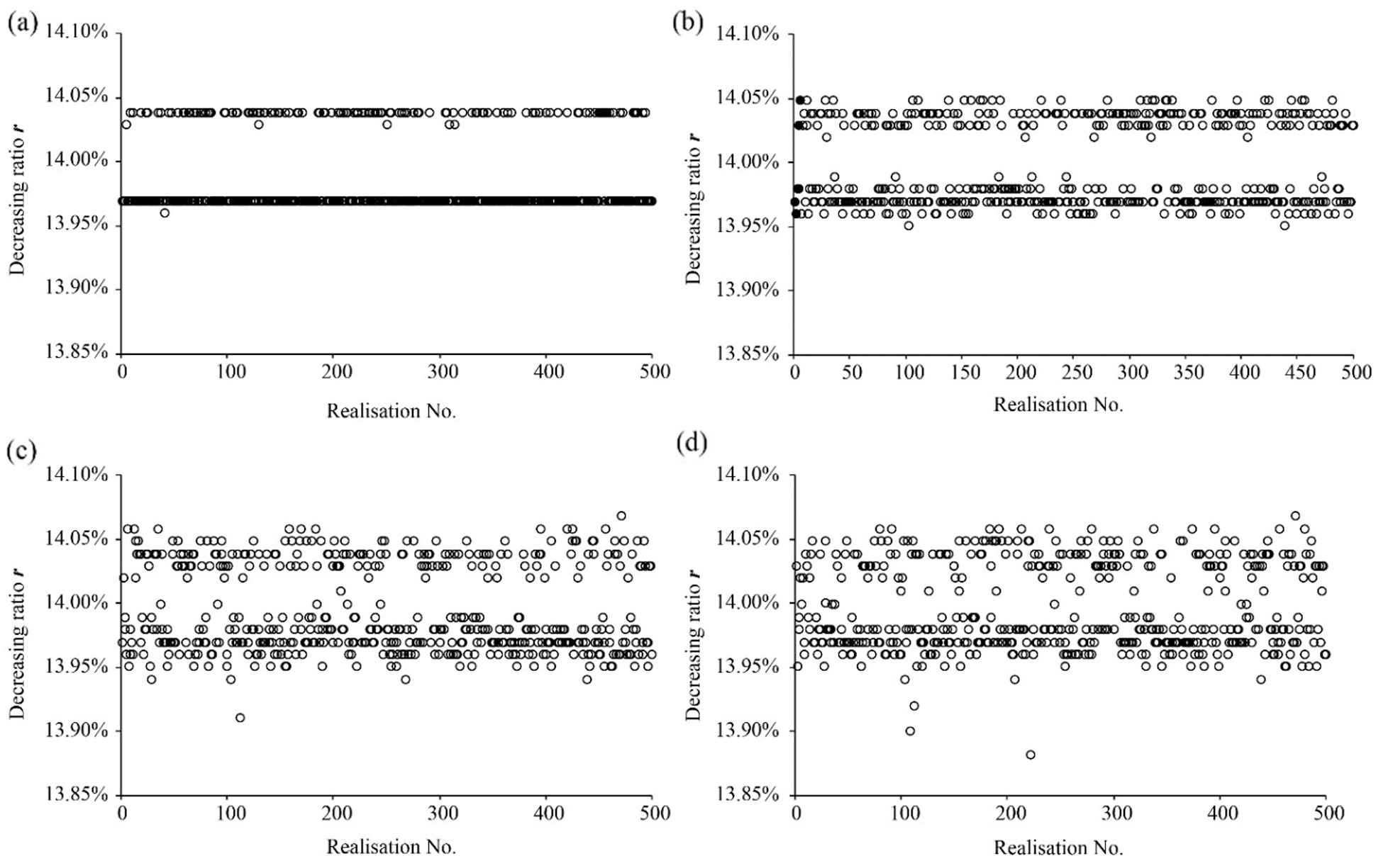
Figure 10: Decreasing ratios of the FOS for the four cases after the 5th freeze-thaw cycle: (a) Case 1; (b) Case 2; (c) Case 3 and (d) Case 4
In this paper, the influence of the heterogeneity in the thermal conductivity on the frozen soil slope stability under the freeze-thaw cycle has been investigated. The coupling behavior between heat and moisture migration is neglected here. The LAS method is used to model the heterogeneity of the thermal conductivity and the strength reduction method is utilized to calculate the FOS of the frozen soil slope. The distribution of the thermal conductivity is assumed to be normal. It has been found that when the temperature is steady, the FOS of the frozen soil slope is influenced by the spatial variability of the thermal conductivity, but the influence is not significant. When the standard deviation and the SOF of the thermal conductivity increase, the mean of the FOS is equal to the FOS of the homogeneous case, and the standard deviation of the FOS also increases. Moreover, with the increase of the standard deviation and the SOF of the thermal conductivity, the distribution of the FOS becomes to be normal.
After the frozen soil goes through freeze-thaw process, firstly, it can be found that the FOS of the frozen soil slope decreases due to the reduction of the cohesion and the internal friction angle caused by the freeze-thaw cycle. When the number of freeze-thaw cycles increases, the reduction of the FOS becomes larger. Furthermore, the decreasing ratio of the FOS becomes more scattered after the 5th freeze-thaw cycle compared to that of the FOS after the 1st freeze-thaw cycle. The larger variability of the FOS could induce inaccuracy in the prediction of the frozen soil slope stability under freeze-thaw cycle.
Funding Statement: The research is supported by the Natural Science Foundation of Anhui Province (Grant No. 1908085QE242); the Fundamental Research Funds for the Central Universities (Grant No. JZ2021HGTB0097); the Natural Science Foundation of China (NSFC) (Grant No. 51908175). The financial support is gratefully acknowledged.
Conflicts of Interest: The authors declare that they have no conflicts of interest to report regarding the present study.
1. Li, S., Lai, Y., Zhang, M., Dong, Y. (2009). Study on long-term stability of qinghai–Tibet railway embankment. Cold Regions Science & Technology, 57(2–3), 139–147. DOI 10.1016/j.coldregions.2009.02.003. [Google Scholar] [CrossRef]
2. Li, S., Lai, Y., Pei, W., Zhang, S., Zhong, H. (2014). Moisture–temperature changes and freeze–thaw hazards on a canal in seasonally frozen regions. Natural Hazards, 72, 287–308. DOI 10.1007/s11069-013-1021-3. [Google Scholar] [CrossRef]
3. Subramanian, S. S., Ishikawa, T., Tokoro, T. (2017). Stability assessment approach for soil slopes in seasonal cold regions. Engineering Geology, 221, 154–169. DOI 10.1016/j.enggeo.2017.03.008. [Google Scholar] [CrossRef]
4. Subcommittee, P. (1988). Glossary of permafrost and related ground-ice terms, pp. 156. Associate Committee on Geotechnical Research, National Research Council of Canada, Ottawa. [Google Scholar]
5. Pei, W., Zhang, M., Li, S., Lai, Y., Jin, L. et al. (2017). Geotemperature control performance of two-phase closed thermosyphons in the shady and sunny slopes of an embankment in a permafrost region. Applied Thermal Engineering, 112, 986–998. DOI 10.1016/j.applthermaleng.2016.10.143. [Google Scholar] [CrossRef]
6. Moghbel, F., Fall, M. (2012). Thermal conductivity of compost biocover subjected to freeze-thaw cycles. 65th Canadian Geotechnical Conference, Winnipeg, Canada. [Google Scholar]
7. Cheng, P. F., Luo, K. Q. (2016). Study on influencing factors and prediction of silty soil thermal conductivity in seasonal frozen area. Science Technology and Engineering, 16(11), 235–239. [Google Scholar]
8. Xiao, Z. H. (2007). Experimental investigation on engineering properties of shanghai soft soils under secondary freeze-thaw action (Master Thesis). Tongji University, China. [Google Scholar]
9. Formanek, G. E., McCCool, D. K., Papendick, R. I. (1984). Freeze–Thaw and consolidation effects on strength of a wet silt loam. Transactions of the American Society of Agricultural Engineers, 27(6), 1749–1752. DOI 10.13031/2013.33040. [Google Scholar] [CrossRef]
10. Graham, J., Au, V. (1985). Effects of freeze–thaw and softening on a natural clay at low stresses. Canadian Geotechnical Journal, 22(1), 69–78. DOI 10.1139/t85-007. [Google Scholar] [CrossRef]
11. Ma, W., Xu, X. Z., Zhang, L. X. (1999). Influence of frost and thaw cycles on shear strength of lime silt. Chinese Journal of Geotechnical Engineering, 21(2), 158–160. [Google Scholar]
12. Hotineanu, A., Bouasker, M., Aldaood, A., Al-Mukhtar, M. (2015). Effect of freeze–thaw cycling on the mechanical properties of lime-stabilized expansive clays. Cold Regions Science & Technology, 119, 151–157. DOI 10.1016/j.coldregions.2015.08.008. [Google Scholar] [CrossRef]
13. Qi, J. L., Ma, W. (2006). Influence of freezing-thawing on strength of overconsolidated soils. Chinese Journal of Geotechnical Engineering, 28(12), 2082–2086. [Google Scholar]
14. Zhou, Z. J., Zhong, S. F., Liang, H. (2013). Test research on change law of highway performance at loess are influenced by number of freeze-thaw cycles. Journal of Chang'an University (Natural Science Edition), 33(4), 1–6. DOI 10.19721/j.cnki.1671-8879.2013.04.001. [Google Scholar] [CrossRef]
15. Yu, L. L., Xu, X. Y., Qiu, M. G., Yan, Z. L., Li, P. F. (2010). Influence of freeze–thaw on shear strength properties of saturated silty clay. Rock and Soil Mechanics, 31(8), 2448–2452. DOI 10.16285/j.rsm.2010.08.052. [Google Scholar] [CrossRef]
16. Lumb, P. (1966). The variability of natural soils. Canadian Geotechnical Journal, 3(2), 74–97. DOI 10.1139/t66-009. [Google Scholar] [CrossRef]
17. Alonso, E. E. (1976). Risk analysis of slopes and its application to slopes in Canadian sensitive clays. Géotechnique, 26(3), 453–472. DOI 10.1680/geot.1976.26.3.453. [Google Scholar] [CrossRef]
18. Wu, T. H., Kraft, L. M. (1970). Safety analysis of slopes. Journal of the Soil Mechanics and Foundations Division, 96(2), 609–630. DOI 10.1061/JSFEAQ.0001406. [Google Scholar] [CrossRef]
19. Cornell, C. (1972). First-order uncertainty analysis of soil deformation and stability. First International Conference on Applications of Probability and Statistics in Soil and Structural Engineering, pp. 129–144. Hong Kong. [Google Scholar]
20. Tang, W., Yucemen, M., Ang, A. S. (1976). Probability-based short term design of soil slopes. Canadian Geotechnical Journal, 13(3), 201–215. DOI 10.1139/t76-024. [Google Scholar] [CrossRef]
21. Vanmarcke, E. H. (1977). Reliability of earth slopes. Journal of the Geotechnical Engineering Division, 103(11), 1247–1265. DOI 10.1061/AJGEB6.0000518. [Google Scholar] [CrossRef]
22. Gui, S., Zhang, R., Turner, J. P., Xue, X. (2000). Probabilistic slope stability analysis with stochastic soil hydraulic conductivity. Journal of Geotechnical and Geoenvironmental Engineering, 126(1), 1–9. DOI 10.1061/(ASCE)1090-0241(2000)126:1(1). [Google Scholar] [CrossRef]
23. Griffiths, D., Fenton, G. A. (2004). Probabilistic slope stability analysis by finite elements. Journal of Geotechnical and Geoenvironmental Engineering, 130(5), 507–518. DOI 10.1061/(ASCE)1090-0241(2004)130:5(507). [Google Scholar] [CrossRef]
24. Liu, K., Vardon, P. J., Hicks, M. A., Arnold, P. (2017). Combined effect of hysteresis and heterogeneity on the stability of an embankment under transient seepage. Engineering Geology, 219, 140–150. DOI 10.1016/j.enggeo.2016.11.011. [Google Scholar] [CrossRef]
25. Liu, K., Wang, Y., Huang, M., Yuan, W. H. (2021). Postfailure analysis of slopes by random generalized interpolation material point method. International Journal of Geomechanics, 21(3), 04021015. DOI 10.1061/(ASCE)GM.1943-5622.0001953. [Google Scholar] [CrossRef]
26. Xu, J., Yang, G., Liu, H. (2007). Evaluation of permafrost slope with monte carlo simulation method and program design. Chinese Journal of Underground Space and Engineering, 3(8), 1433–1437. [Google Scholar]
27. Zhang, Z. (2009). The variability of frozen-soil parameters and its applying in slope reliability analysis (Master Thesis). Xi'an University of Science and Technology, China. [Google Scholar]
28. Li, T., Guo, L., Li, W., Wang, F. (2010). Reliability analysis of slope stability under the condition of extreme ice-snow and frozen disaster. Proceedings of 12th Biennial International Conference on Engineering, Construction, and Operations in Challenging Environments and Fourth NASA/ARO/ASCE Workshop on Granular Materials in Lunar and Martian Exploration, pp. 2975–2982. Honolulu, USA. [Google Scholar]
29. Guo, L., Li, T., Liu, X., Niu, Z. (2011). Reliability analysis of slope under conditions of extreme snow disaster. Water Resources and Power, 29(8), 103–105+213. [Google Scholar]
30. Chen, X., Liu, J. K., Xie, N., Sun, H. J. (2015). Probabilistic analysis of embankment slope stability in frozen ground regions based on random finite element method. Sciences in Cold and Arid Regions, 7(4), 354–364. DOI 10.3724/SP.J.1226.2015.00354. [Google Scholar] [CrossRef]
31. Haigh, G. H. (2012). Thermal conductivity of sands. Géotechnique, 62(7), 617–625. DOI 10.1680/geot.11.P.043. [Google Scholar] [CrossRef]
32. Zhang, N., Xia, S. Q., Hou, X. Y., Wang, Z. Y. (2016). Review on soil thermal conductivity and prediction model. Rock and Soil Mechanics, 37(6), 1550–1562. DOI 10.16285/j.rsm.2016.06.004. [Google Scholar] [CrossRef]
33. Wang, T., Zhou, G., Wang, J., Zhao, X., Yin, Q. et al. (2015). Stochastic analysis model of uncertain temperature characteristics for embankment in warm permafrost regions. Cold Regions Science and Technology, 109, 43–52. DOI 10.1016/j.coldregions.2014.09.013. [Google Scholar] [CrossRef]
34. Wang, T., Zhou, G., Wang, J., Zhao, X. (2016). Stochastic analysis for the uncertain temperature field of tunnel in cold regions. Tunnelling and Underground Space Technology, 59, 7–15. DOI 10.1016/j.tust.2016.06.009. [Google Scholar] [CrossRef]
35. Zhu, Z., Ning, J., Song, S. (2010). Finite-element simulations of a road embankment based on a constitutive model for frozen soil with the incorporation of damage. Cold Regions Science and Technology, 62, 151–159. DOI 10.1016/j.coldregions.2010.03.010. [Google Scholar] [CrossRef]
36. Anderson, D. M., Tice, A. R. (1973). The unfrozen interfacial phase in frozen soil water systems. Ecological Study: Analysis and Synthesis, 4, 107–124. [Google Scholar]
37. Xu, X. Z., Wang, J. C., Zhang, L. X. (2010). Physics of frozen soil. China: Science Press. [Google Scholar]
38. van Genuchten, M. T. (1980). A closed-form equation for predicting the hydraulic conductivity of unsaturated soils. Soil Science Society of America Journal, 44(5), 892–898. DOI 10.2136/sssaj1980.03615995004400050002x. [Google Scholar] [CrossRef]
39. Mualem, Y. (1976). A new model for predicting the hydraulic conductivity of unsaturated porous media. Water Resources Research, 12(3), 513–522. DOI 10.1029/WR012i003p00513. [Google Scholar] [CrossRef]
40. Fenton, G. A. (1994). Error evaluation of three random-field generators. Journal of Engineering Mechanics, 120(12), 2478–2497. DOI 10.1061/(ASCE)0733-9399(1994)120:12(2478). [Google Scholar] [CrossRef]
41. Samy, K. (2003). Stochastic analysis with finite elements in geotechnical engineering (Ph.D. Thesis). University of Manchester, UK. [Google Scholar]
42. Spencer, W. A. (2007). Parallel stochastic and finite element modelling of clay slope stability in 3D (Ph.D. Thesis). University of Manchester, UK. [Google Scholar]
43. Smith, I. M., Griffiths, D. V., Margetts, L. (2014). Programming the finite element method (Fifth Edition). West Sussex, UK: Wiley. [Google Scholar]
44. Chen, X., Liu, J. K., Feng, Y., Li, X., Tian, Y. H. et al. (2013). A pseudo-coupled numerical approach for stability analysis of frozen soil slopes based on finite element limit analysis method. Sciences in Cold and Arid Regions, 5(4), 478–487. DOI 10.3724/SP.J.1226.2013.00478. [Google Scholar] [CrossRef]
45. Chen, Y., Wu, P., Yu, Q., Xu, G. (2017). Effects of freezing and thawing cycles on mechanical properties and stability of soft rock slope. Advances in Material Science and Engineering, 2017, 3173659. DOI 10.1155/2017/3173659. [Google Scholar] [CrossRef]
46. Usowicz, B., Kossowski, J., Baranowski, P. (1996). Spatial variability of soil thermal properties in cultivated fields. Soil and Tillage Research, 39(1–2), 85–100. DOI 10.1016/S0167-1987(96)01038-0. [Google Scholar] [CrossRef]
47. Ferguson, G. (2010). Heterogeneity and thermal modeling of ground water. Groundwater, 45(4), 485–490. DOI 10.1111/j.1745-6584.2007.00323.x. [Google Scholar] [CrossRef]
48. Simms, R. B., Haslam, S. R., Craig, J. R. (2014). Impact of soil heterogeneity on the functioning of horizontal ground heat exchangers. Geothermics, 50, 35–43. DOI 10.1016/j.geothermics.2013.08.007. [Google Scholar] [CrossRef]
 | This work is licensed under a Creative Commons Attribution 4.0 International License, which permits unrestricted use, distribution, and reproduction in any medium, provided the original work is properly cited. |