| Computer Modeling in Engineering & Sciences |
DOI: 10.32604/cmes.2022.018325
ARTICLE
Comparative Study on Deformation Prediction Models of Wuqiangxi Concrete Gravity Dam Based on Monitoring Data
1Hunan Wuling Power Technology Corporation Ltd., Changsha, 410004, China
2Wuling Power Corporation Ltd., Changsha, 410004, China
3Nanjing Research Institute of Hydrology and Water Conservation Automation, Ministry of Water Resources, Nanjing, 210012, China
4Department of Engineering Mechanics, Hohai University, Nanjing, 211100, China
*Corresponding Author: Tiantang Yu. Email: tiantangyu@hhu.edu.cn
Received: 28 July 2021; Accepted: 14 October 2021
Abstract: The deformation prediction models of Wuqiangxi concrete gravity dam are developed, including two statistical models and a deep learning model. In the statistical models, the reliable monitoring data are firstly determined with Lahitte criterion; then, the stepwise regression and partial least squares regression models for deformation prediction of concrete gravity dam are constructed in terms of the reliable monitoring data, and the factors of water pressure, temperature and time effect are considered in the models; finally, according to the monitoring data from 2006 to 2020 of five typical measuring points including J23 (on dam section
Keywords: Wuqiangxi concrete gravity dam; deformation prediction; stepwise regression model; partial least squares regression model; LSTM model
During the service period, dams not only bear various cyclic loads and sudden disasters, but also suffer from erosion and corrosion from harsh environment, and it leads to the gradual decline of local and overall safety performance. Once the dam is wrecked, it will yield disastrous consequences. Therefore, it is very important to identify the potential risk and evaluate dam safety behavior in time based on the dam monitoring data collected by prototype observation instruments.
The traditional analysis models for dam deformation monitoring data include statistical model [1,2], deterministic model [3] and hybrid model [4–6] and combination model [7,8]. The idea of statistical model is to establish the relationship between environmental variables (such as, water level, temperature, aging, etc.) and the effect variables (such as, deformation, seepage, cracking, etc.) by modeling and analyzing the monitoring data based on probability theory and mathematical statistics theory. The statistical model can simulate structural changes and predict its development trend, its implementations are simple, and its accuracy can meet engineering requirements, so the statistical model has been widely used in engineering. In the deterministic model, the displacement, stress, seepage fields, etc. of the dam and foundation under load are calculated with numerical mehods such as finite element method (FEM) [9], extended finite element method (XFEM) [6,10], meshfree methods [11], etc.; and then some parameters are adjusted by optimizing the fitting between the calculated values and the measured values; thus the expression based on the essence of physics and mechanics can be established. The shortcomings of the deterministic model are uncertainty of dam and foundation material parameters, inaccuracy in setting boundary conditions and inaccuracy of model simplification. Hybrid model uses numerical mehods to calculate water pressure component, and other components are obtained with the statistical model, and then the obtained values are optimally fitted with the measured values. Although the hybrid model improves the calculation accuracy from the mechanics concept, it also inherits the inherent defects and assumptions of statistical model and deterministic model. Combined model performs nonlinear optimization combination on multiple single models by integrating various useful information to achieve a more reasonable and comprehensive description of mapping relationship, and it can effectively improve fitting and prediction accuracy. The shortcomings of the combination model include: (1) the linear combination model may get unrealistic negative weights for dealing with nonlinear problems; (2) it is very difficult to construct combinatorial functions.
Li et al. [12] reviewed the dam monitoring data analysis methods including the monitoring models, monitoring indices, and anomaly value detection methods. Tonini [13] first applied a cubic polynomial to describe the water pressure and temperature components using statistical analysis. Wu [14] investigated the selection of environmental variables and the corresponding mechanisms by combining dam theory, statistical theory and engineering mechanics, and deduced mathematical models of the water pressure and temperature components. Chen [15] proposed exponential function, hyperbolic function, and logarithmic function models for time-dependent component of a concrete dam based on creep theory. Léger et al. [16] presented frequency domain solution algorithms of the one-dimensional transient heat transfer equation for describing temperature variations in arch dam cross sections, thus the temperature variations are not required to be specified at the upstream and downstream faces. Tatin et al. [17] developed a hybrid physico-statistical model to improve the assessment of displacements due to the temperature field in a dam, and cases show that the improved assessment of thermal effects on reversible phenomena leads to a reduced uncertainty on residuals. Mata et al. [18] presented a methodology for the selection of the thermometers that best represent the thermal effect in the statistical model. Hu et al. [1] proposed the special statistical models for the displacements of high arch dams during their initial impoundment periods by improving estimations of the non-stationary thermal and the non-monotonic timedependent effects. Wang et al. [19] presented a shape feature-based spatial clustering method for the dam temperature field, and established a displacement monitoring model of concrete dams using the shape feature clustering-based temperature principal component factor.
Stepwise regression and partial least squares regression are widely used in statistical models. In stepwise regression model, environmental variables are added to the model one by one, and the significance of environmental variables to the model is sequentially assessed to obtain the optimal variable set. Hu et al. [20] established the stepwise regression model of Bikou earth-rockfill dam deformation displacement based on the least squares method of statistics principles, and the results show that the model has higher fitting precision and longer predict cycle. Shen et al. [21] studied the influences of factors on gravity dam open crack with multiple stepwise regression method. The partial least squares method extracts the principal components from the set of independent variables, and the extracted principal components are linearly independent. However, when the extracted components contain significant amounts of information that is unrelated to the dependent variables, the results of the partial least squares method are not satisfactory [22]. Cheng et al. [23] proposed an improved observation method and improved partial least squares data analysis methods to overcome the shortcomings of the traditional methods of external deformation monitoring and data analysis of high rock-fill dams. Yin et al. [24] proposed a novel nonlinear component separation method for the effect quantities by combining kernel partial least squares and pseudosamples, and the separated displacement components of a super-high arch dam conform to the general deformation law. Considering the characteristics of complex nonlinear and multiple response variables of a super-high dam, a universal unified optimization algorithm was developed to select the kernel partial least squares parameters and achieve the optimal kernel partial least squares [25]. With the development of statistical regression, some regression models have been gradually introduced into dam safety monitoring, such as threshold regression [26], logistic regression [27] and random forest regression [28,29], etc. The multicollinearity among environmental variables and the effective optimization of the model are two key issues which affect the quality of a statistical model.
In recent years, with the development of dam safety monitoring, computer, big data, artificial intelligence and other theories and technologies, more and more data mining methods have been applied to the dam safety monitoring modeling, and many intelligent algorithm monitoring models have emerged, and these models show unique advantages in solving the problems of uncertainty and nonlinearity of monitoring model factors, prediction accuracy and generalization. Qu et al. [30] established single-point and multipoint concrete dam deformation prediction models based on long short-term memory (LSTM) network, and proposed a new evaluation system and quantitative evaluation indexes. Yang et al. [31] proposed a concrete dam deformation prediction method based on LSTM with attention mechanism, which can effectively avoid the gradient disappearance and gradient explosion problems in the recurrent neural network. Liu et al. [32] predicted long-term displacements of arch dams by combining the LSTM network and dimension reduction methods, and the results reveal that the coupling prediction models have higher accuracy and can capture the long-term characteristics of the arch dam deformation. Han et al. [33] predicted the horizontal displacement of concrete-face rockfill dams using the statistically optimized back-propagation neural network model, which can overcome the shortcomings of the statistical model and back-propagation neural network model. Chen et al. [34] proposed a novel deformation prediction model of arch dam via correlated multi-target stacking. Shi et al. [35] developed a safety monitoring model for concrete face rockfill dam seepage with cracks considering the lagging effect using the radial basis function neural network. Yang et al. [36] presented an intelligent singular value diagnostic method based on convolutional neural network for concrete dam deformation monitoring. Liu et al. [37] investigated the applicability of the kernel-extreme learning machines-based model considering the thermal effect on the behavior prediction of concrete arch dams. Chen et al. [38] builded the structural health monitoring framework of concrete dam displacement and mined the effects of hydrostatic, seasonal and irreversible time components on dam deformation by combining with relevance vector machine, multi-kernel technique, hydrostatic-season-time statistical model and parallel Jaya algorithm. Shu et al. [39] proposed a novel prediction model based on variational autoencoder and temporal attention-based long short-term memory network for the long-term deformation of arch dams. Chen et al. [40] developed an integrated displacement prediction method based on the spatiotemporal clustering and machine learning algorithms.
This study aims to establish the deformation prediction models of Wuqiangxi concrete gravity dam based on the monitoring data. According to the monitoring data from 2006 to 2020 of measuring points J23 (on dam section
After the introduction, the statistical models and LSTM model for deformation prediction of concrete gravity dam are described in Sections 2 and 3, respectively. Case studies and discussion are given in Section 4. Some conclusions are obtained in Section 5.
2 Statistical Models for Deformation Prediction of Concrete Gravity Dam
The monitoring data are independent, and are easily affected by environmental factors in the process of observation, resulting in some monitoring data that do not conform to the regular changes, which are unreliable data. In order to improve the prediction performance of statistical model, the unreliable data should be removed.
Generally, the reliability of data is judged by Lahitte criterion (also called 3
where yi is the ith monitoring data.
Assume that n monitoring data are known,
The ratio of absolute value of runout deviation and mean square deviation of the ith monitoring data is defined as
As qi > 3, it indicates that the monitoring data is abnormal or unreliable, and it should be removed.
The displacement vector at one point in dam can be divided into horizontal displacement
where
The displacement component at one point in the concrete gravity dam under water pressure and reservoir water weight can be described as [14]
where a1i and a2i are the regression coefficients of upstream and downstream water pressure factors, respectively. H is the upstream depth, and h is the downstream water depth.
After some years of dam operation, the temperature inside the dam reaches the quasi-stable temperature field, so it can be assumed that the internal temperature of the dam body is only affected by the water temperature and air temperature, the water temperature and air temperature change harmoniously, and the deformtion is linearly related to the temperature of concrete. The temperature component is expressed as [14]
where b1 and b2 are the regression coefficients of temperature factor, t is the cumulative number of days from the corresponding monitoring day to the inital monitoring day.
At the beginning of impoundment, the aging displacement generally changes violently, and then tends to be stable. The aging component can be expressed as [14]
where c1 and c2 are the regression coefficients of aging factor, and
Substituting Eqs. (5)–(7) into Eq. (4) yields
2.2.1 Stepwise Regression Method
The stepwise regression method [20,21] starts with an independent variable, then independent variable is introduced into the regression equation one by one based on the effect of the independent variable, and the independent variable which has large effect is first introduced into regression equation. On the other hand, when the first introduced independent variables become insignificant due to the introduction of the latter independent variables, they are removed from the regression equation at any time. Therefore, the so-called step-by-step is to introduce independent variables at some steps, and eliminate independent variables at some steps. At each step, F test is done to ensure that the regression equation only contains independent variables with significant effect before introducing new significant independent variables. When all the independent variables with significant effect are contained in the regression equation, the equation is the final regression equation.
There are k independent variables, and n groups of monitoring data series about the independent variables
with
where
In order to solve regression coefficients
where
The process of solving Eq. (12) using stepwise regression method is to change
In order to objectively evaluate the application of stepwise regression method to dam deformation prediction, the multiple correlation coefficient (MCC) and residual standard deviation (RSD) are used as the evaluation indexes of prediction accuracy. The MCC and RSD are defined as
where
where m is the number of eliminating-introducing.
The bigger the value of MCC, the better the prediction accuracy. The smaller the value of RSD, the better the prediction accuracy.
2.2.2 Partial Least Squares Regression Method
Partial least squares regression [23,25] is the regression of multiple dependent variables to multiple independent variables. There are q dependent variables, i.e.,
3 LSTM Model for Deformation Prediction of Concrete Gravity Dam
Long short-term memory (LSTM) network is a kind of back propagation recurrent neural network. In the LSTM [31], the concept of time series is introduced into the network structure to mine the association between long-term and short-term deformation monitoring data. By improving the simple node of traditional neural network into a storage unit, the problem of gradient disappearance and gradient explosion when learning the association of long-term and long-term data is avoided, and the prediction accuracy is improved. The LSTM can remember information, also known as a cell. The main excellent features of the LSTM are as follows: (1) it can learn the complex nonlinear relationship between effect sets and load sets through training; (2) it can selectively retain the previous deformation and the corresponding load when calculating the deformation under the current load; (3) it has the memorability and can learn the laws between the deformation and the previous load set.
3.2 Selection of the Hyper-Parameters
In general, the hyper-parameters involved in the training of recurrent neural network are selected according to experience. However, the LSTM recurrent neural network is sensitive to the selection of hyper-parameters in training. In order to achieve better results, the optimization algorithm is adopted to optimize the hyper-parameters. The optimization of network hyper-parameters mainly focuses on three parameters: sample length, the number of hidden neurons in feedforward network layer (also known as state vector size), the learning rate which controls the adjustment range of network parameter. The grid search algorithm and random search algorithm are widely used to optimize the hyper-parameters of LSTM recurrent neural network.
Grid search determines the spatial dimension of grid search according to the number of hyper-parameters, divides the grid on each dimension, then determines the best hyper-parameters according to the results given by grid intersections. The search process of grid search is mainly divided into three steps: first, the values of less important hyper-parameters are fixed; second, the range of three hyper-parameters are set; finally, the target function LSTM recurrent neural network test set is set to the highest recognition accuracy. The existing studies show that the method based on grid search can obtain high precision result, but the computing cost increases exponentially with the increase of the number of hyper-parameters.
The search space of random search cannot be discrete, which allows random search to try more hyper-parameter combinations under the same computing resources. Grid search wastes a lot of computing resources in the hyper-parameters which have little impact on the network performance, while random search tests the unique value of each hyper-parameter which has an impact on the results almost every time, that is to say, random search tries more beneficial hyper-parameter combinations. Random search can greatly shorten the search time and improve the computational efficiency on the premise of ensuring a certain accuracy. After selecting the optimized super parameters, the recognition accuracy of LSTM recurrent neural network is greatly improved.
In this study, the LSTM recurrent neural network coupled with random search is used to construct the deformation prediction model of concrete gravity dam.
In order to objectively evaluate the application of LSTM model to dam deformation prediction, the root mean square error (RMSE) is used as the evaluation index of prediction accuracy. The RMSE is defined as
where n is the number of forecast data; yi is the true value of the ith data of the prediction group;
Wuqiangxi hydropower station which was completed in 1999 is located in the middle and upper reaches of the main stream of the Yuan River in Hunan province, China, as shown in Fig. 1. The project is mainly composed of three parts: the river blocking dam, the powerhouse behind the dam on the right bank and the three-stage ship lock on the left bank. Fig. 2 presents the schematic diagram of layout of Wuqiangxi hydropower station, and Figs. 3 and 4 are the upstream and downstream views.
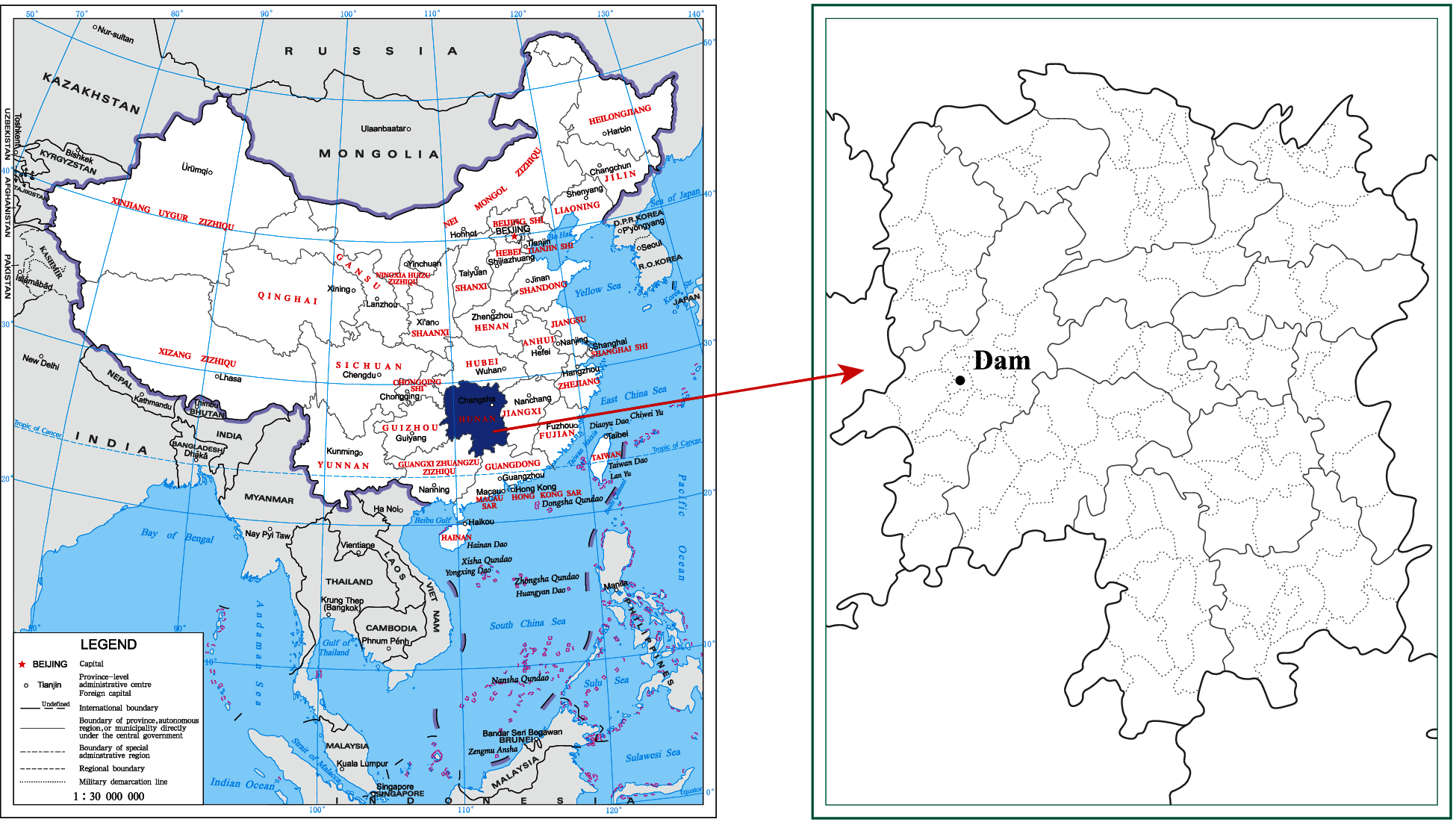
Figure 1: Location of Wuqiangxi hydropower station (the longitude and latitude of the dam are 110.6294 and 28.5783, respectively)
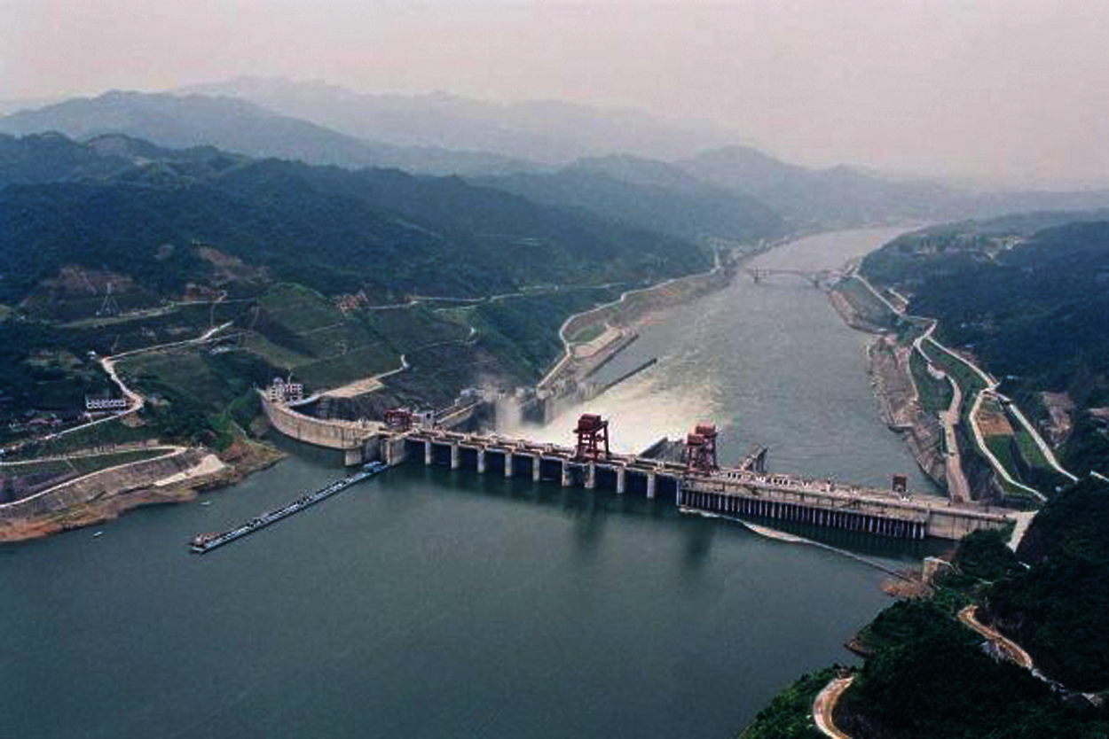
Figure 2: Wuqiangxi hydropower station
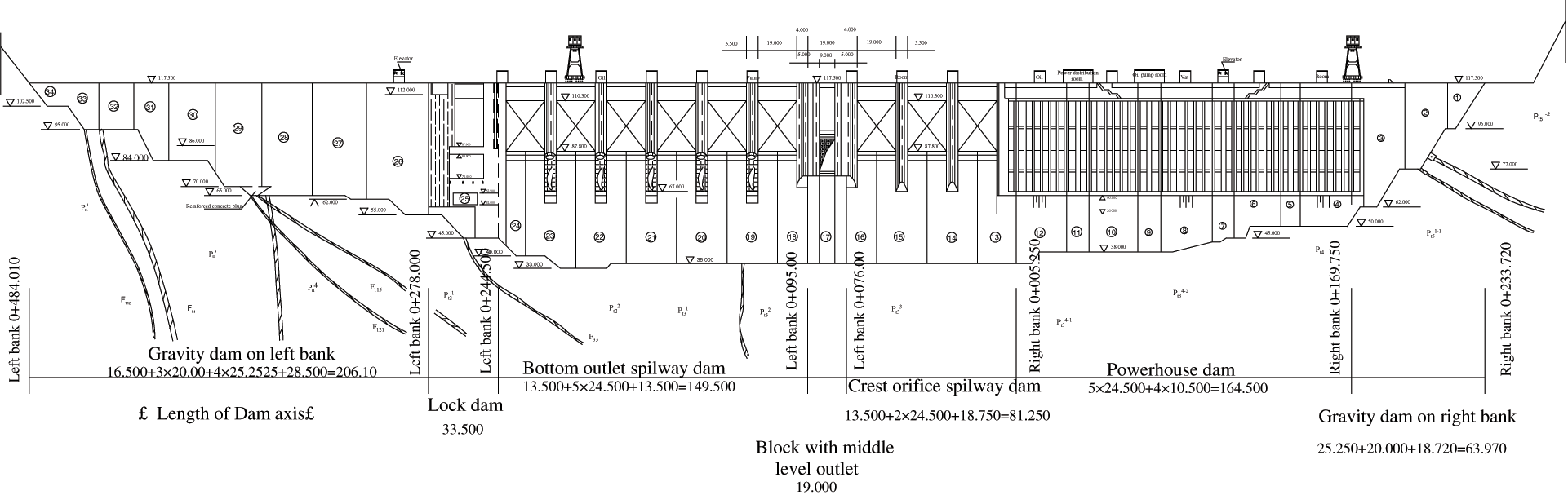
Figure 3: View of the upstream of the junction (scale:1:5000)
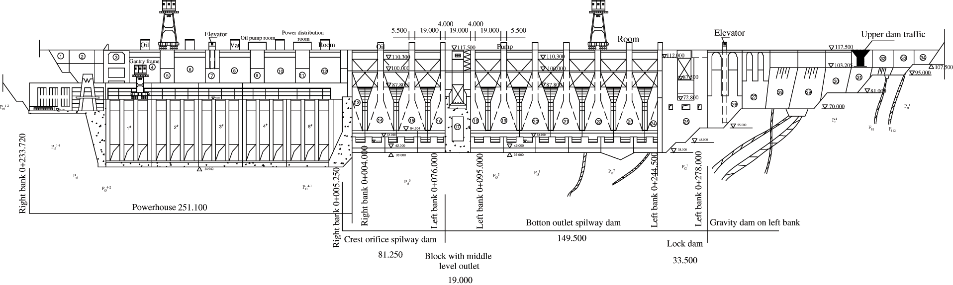
Figure 4: View of the downstream of the junction (scale:1:5000)
The dam is a concrete gravity dam. The crest elevation is 117.5 m, the highest dam height is 85.83 m, and the total crest length is 719.7 m. The main dam is divided into 34 dam sections, including the right bank retaining dam sections ,
There are 51 measurement points of the hydrostatic leveling instrument on the dam crest, numbered J J47, as shown in Fig. 5. Two measurement points of the hydrostatic leveling instrument are arranged at dam sections
The hydrostatic leveling system on the dam crest is based on J0 on the right bank, and double metal markers SJ1 and SJ2 are embedded in this part. Based on the monitoring data of measuring points J23 (on dam section
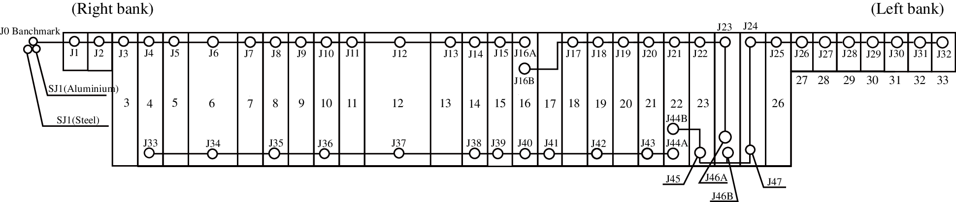
Figure 5: Schematic diagram of hydrostatic leveling layout of dam crest
The unreliable monitoring data of vertical displacements are determined with the Lahitte criterion. Table 1 shows the unreliable subsidence monitoring data of J23. Fig. 6 presents the process line of measured vertical displacements of J23. After removing the unreliable monitoring data, the subsidence process line of J23 is smoother.
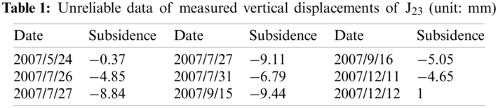
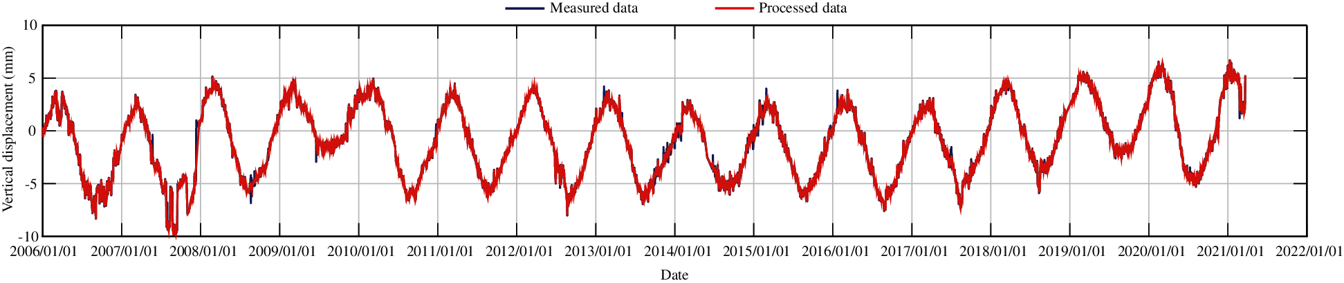
Figure 6: The process line of measured vertical displacements of J23 (unit: mm)
4.3 Statistical Regression Models
For convenience of expression, Eq. (8) can be rewritten as
where
4.3.1 Partial Least Squares Regression Model
In the cross-validity analysis of measuring point J23 from 2006 to 2020,
The regression equation of standardized displacement variable is written as
By reducing standardized variables to original variables, the regression equation of partial least squares method is obtained as follows
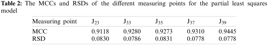
The multiple correlation coefficients (MCCs) and the residual standard deviations (RSDs) of the different measuring points for the partial least squares model are given in Table 2. The MCCs of the five measuring points on different dam sections exceed 0.91, and the RSDs do not exceed 0.0831. It shows that the high accuracy can be obtained with the partial least squares model.
Figs. 7, 9, 11, 13, and 15 show the fitting curve of J23, J33, J35, J37 and J39 obtained with the partial least squares model, respectively. Figs. 8, 10, 12, 14 and 16 present the process line of each component of J23, J33, J35, J37 and J39, respectively. It can be seen that this model can better reflect the variation law of dam crest settlement.
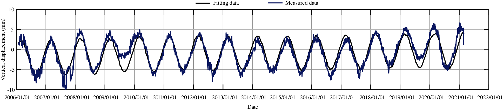
Figure 7: The fitting curve of vertical displacement for measuring point J23 by partial least squares method
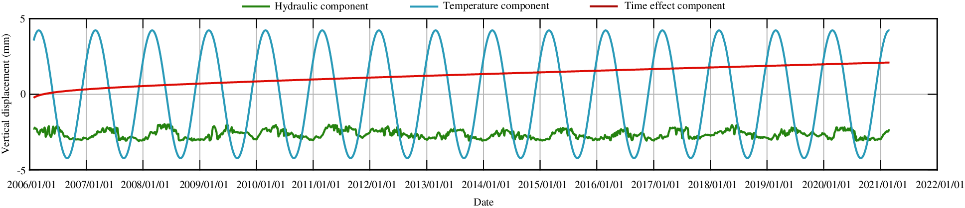
Figure 8: The process line of each component of vertical displacement for measuring point J23 by partial least squares method
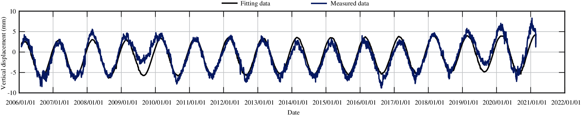
Figure 9: The fitting curve of vertical displacement for measuring point J33 by partial least squares method
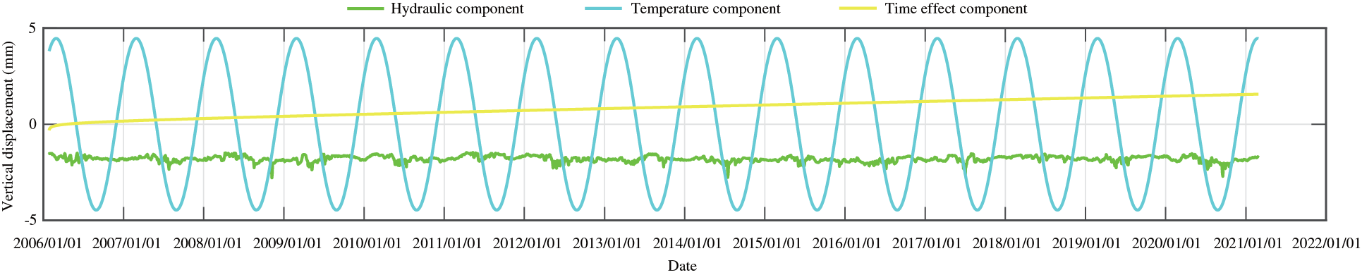
Figure 10: The process line of each component of vertical displacement for measuring point J33 by partial least squares method
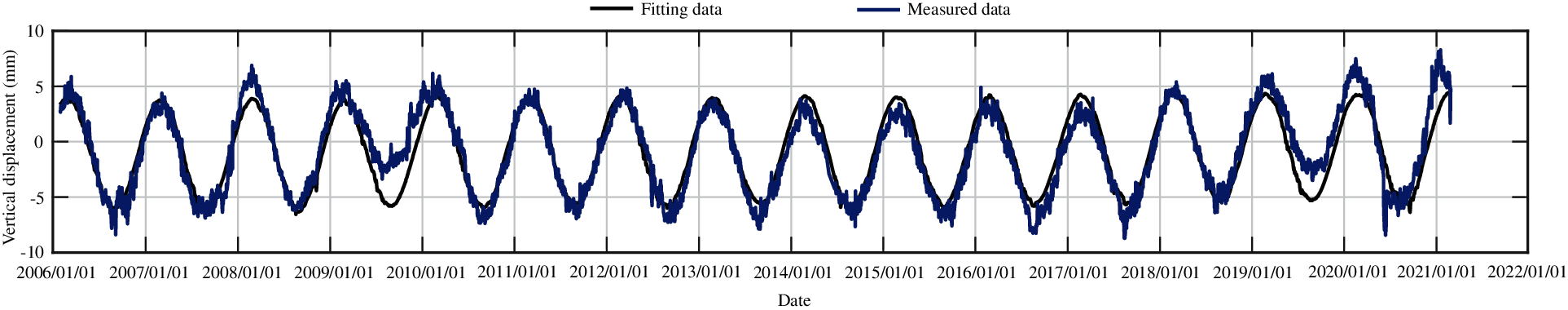
Figure 11: The fitting curve of vertical displacement for measuring point J35 by partial least squares method
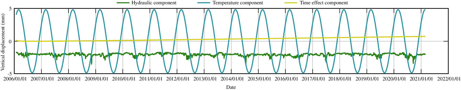
Figure 12: The process line of each component of vertical displacement for measuring point J35 by partial least squares method
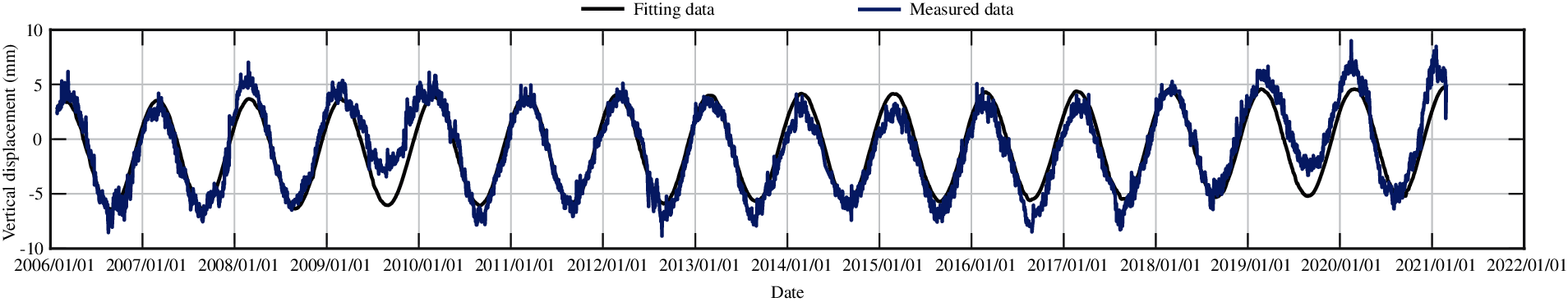
Figure 13: The fitting curve of vertical displacement for measuring point J37 by partial least squares method
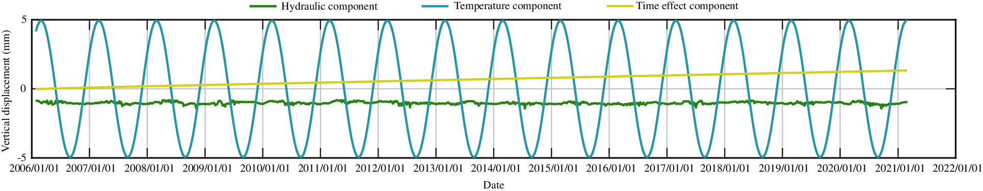
Figure 14: The process line of each component of vertical displacement for measuring point J37 by partial least squares method
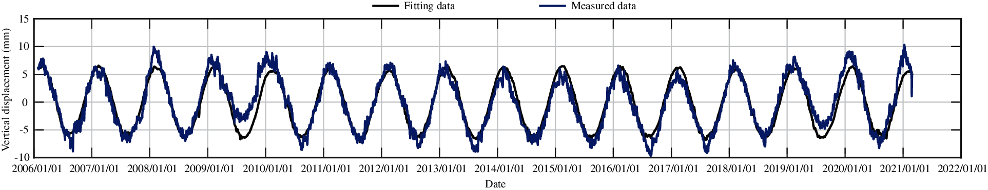
Figure 15: The fitting curve of vertical displacement for measuring point J39 by partial least squares method
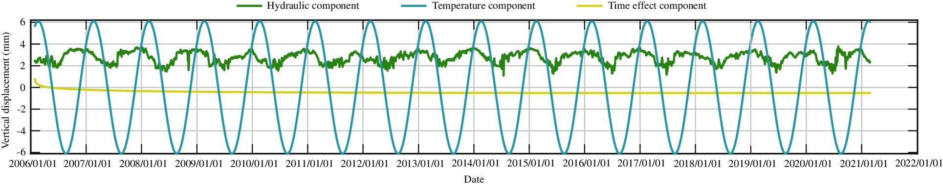
Figure 16: The process line of each component of vertical displacement for measuring point J39 by partial least squares method
4.3.2 Stepwise Regression Model
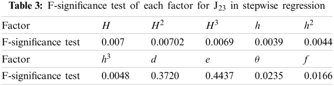
Table 3 shows the F-significance test of each factor for J23 with stepwise regression method, showing the significance level of each factor. According to the significance level of the factors, the stepwise regression equation can be obtained by introducing variables in turn.
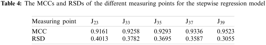
The multiple correlation coefficients (MCCs) and the residual standard deviations (RSDs) of the different measuring points for the stepwise regression model are given in Table 4. The MCCs of the five measuring points on different dam sections exceed 0.91, and the RSDs do not exceed 0.4013. It shows that the high accuracy can be also obtained with the stepwise regression model.
Figs. 17, 19, 21, 23 and 25 show the fitting curve of J23, J33, J35, J37 and J39 obtained with stepwise regression model, respectively. Figs. 18, 20, 22, 24 and 26 show the process line of each component of J23, J33, J35, J37 and J39, respectively.
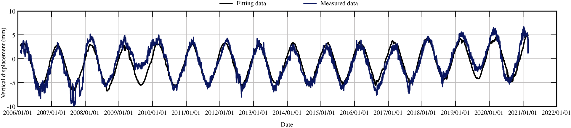
Figure 17: The fitting curve of vertical displacement for measuring point J23 by stepwise regression model
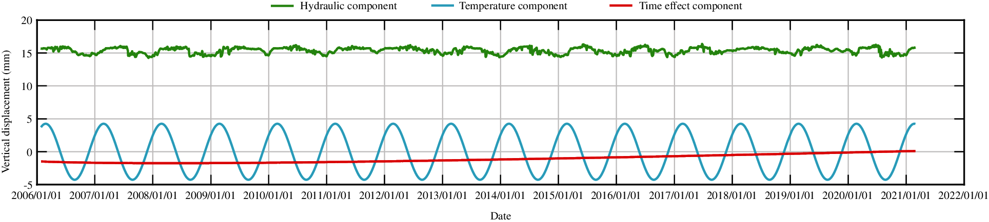
Figure 18: The process line of each component of vertical displacement for measuring point J23 by stepwise regression model
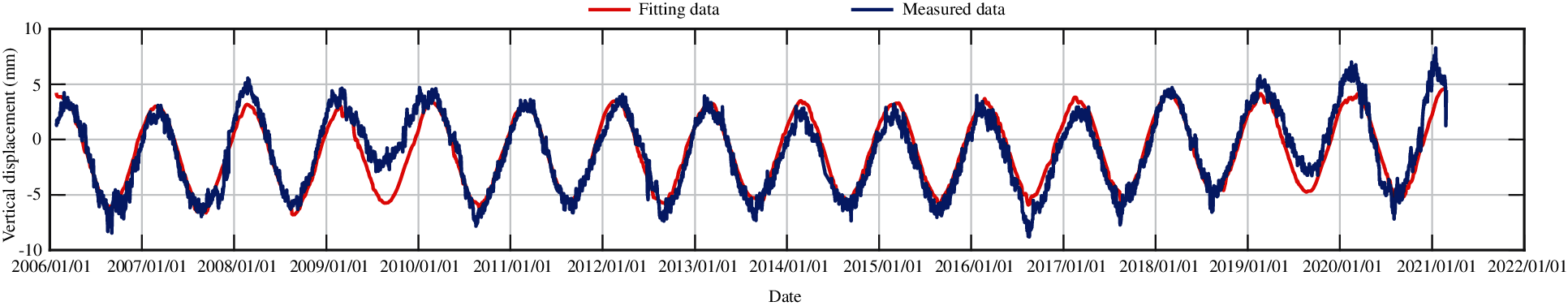
Figure 19: The fitting curve of vertical displacement for measuring point J33 by stepwise regression model
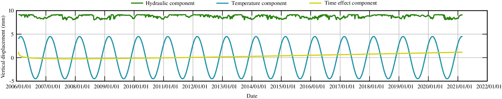
Figure 20: The process line of each component of vertical displacement for measuring point J33 by stepwise regression model
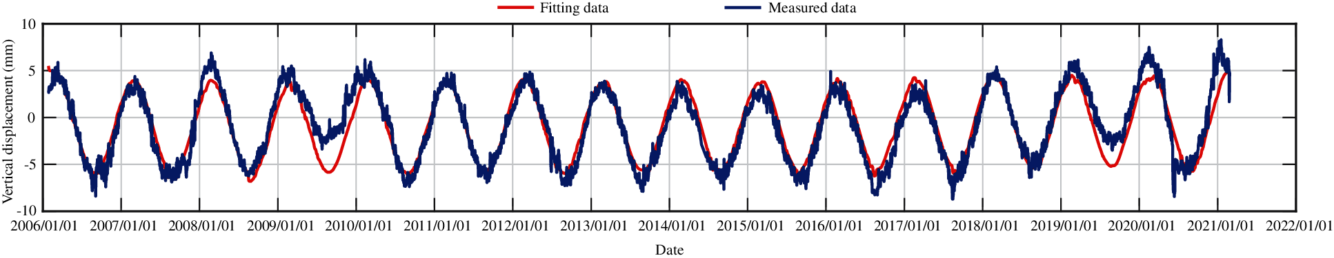
Figure 21: The fitting curve of vertical displacement for measuring point J35 by stepwise regression model
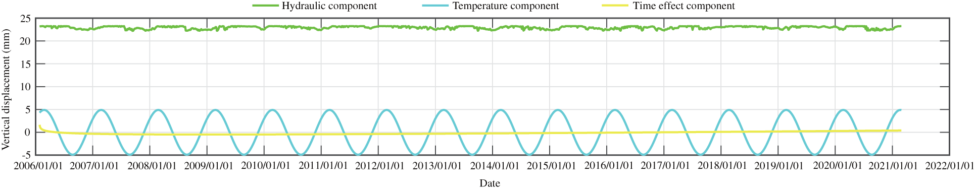
Figure 22: The process line of each component of vertical displacement for measuring point J35 by stepwise regression model
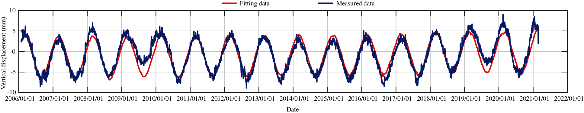
Figure 23: The fitting curve of vertical displacement for measuring point J37 by stepwise regression model
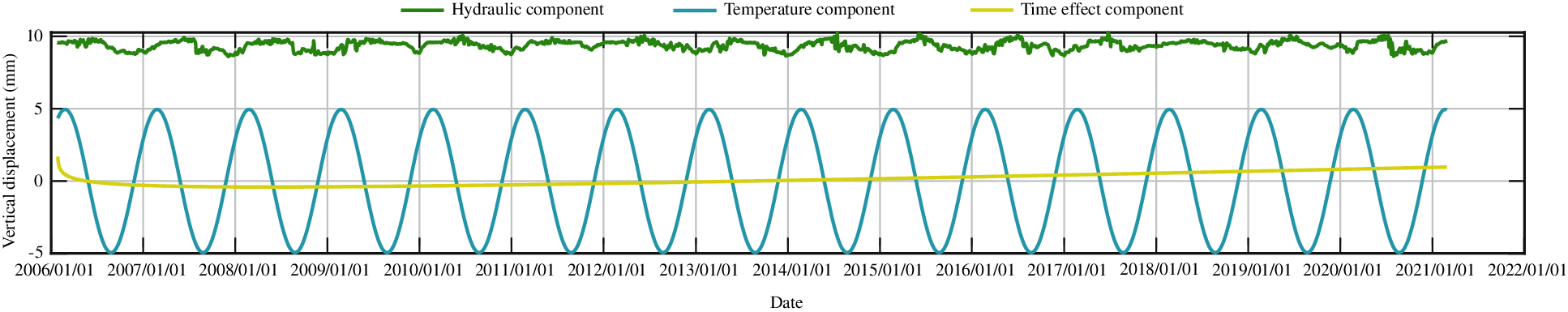
Figure 24: The process line of each component of vertical displacement for measuring point J37 by stepwise regression model
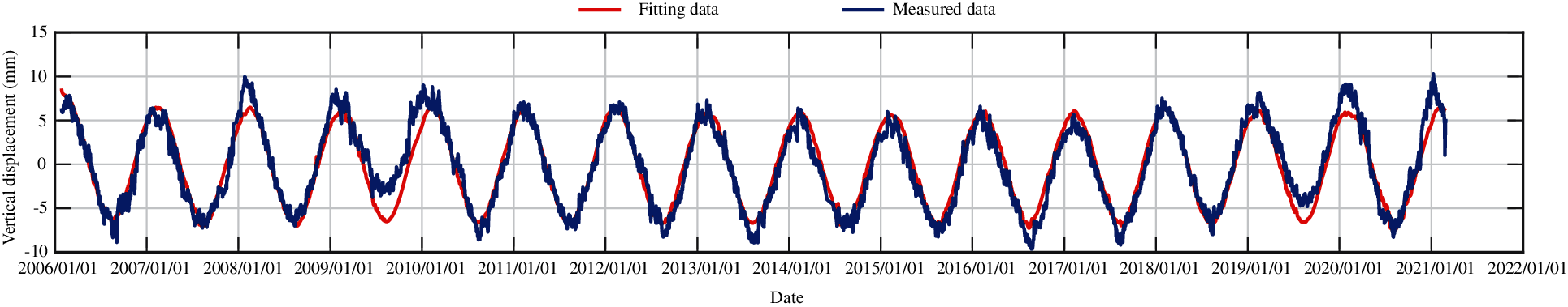
Figure 25: The fitting curve of vertical displacement for measuring point J39 by stepwise regression model
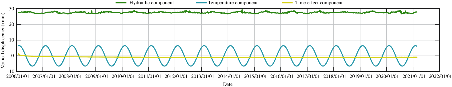
Figure 26: The process line of each component of vertical displacement for measuring point J39 by stepwise regression model
From Figs. 8 and 18, an offset can be found in the hydraulic component when comparing the different statistical models. The stepwise regression and partial least squares regression have no physical meaning, they only fit the data with different ways. The variable substitution is conducted in the partial least squares method, so the components in the partial least squares model are not equivalent to those in the stepwise regression model. In sum, there is no equivalence between the two models.
According to the numerical experiments, two LSTM layers are used, the rectified linear unit function is adopted as the activation function, and the input sequence length is 20, that is, the subsidence data of the first 20 days are used to predict the subsidence of the 21st day. The monitoring data of the training set are from 2006 to 2017, and the monitoring data from 2018 to 2020 are taken as the test set. The RMSEs of the trained model in the training set and in the test set for different measuring points are shown in Table 5. Figs. 27–31 present the training set and the test set of vertical displacement for measuring points J23, J33, J35, J37 and J39 by LSTM method. The RMSEs of measuring point J23 in the training set and in the test set for different training datasets are shown in Table 6, and the corresponding training set and test set of vertical displacement from the trained model are shown in Figs. 32 and 33. The accuracy of the model increases with the increase of the training dataset. In addition, it is found that the accuracy of the predictions are very high when the training data are enough.
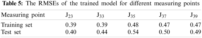
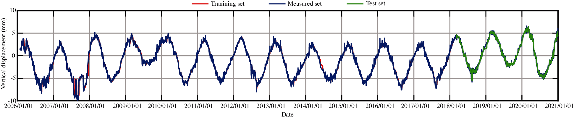
Figure 27: The training set and the test set of vertical displacement for measuring point J23 by LSTM method
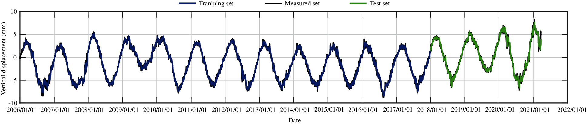
Figure 28: The training set and the test set of vertical displacement for measuring point J33 by LSTM method
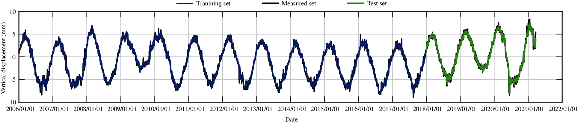
Figure 29: The training set and the test set of vertical displacement for measuring point J35 by LSTM method
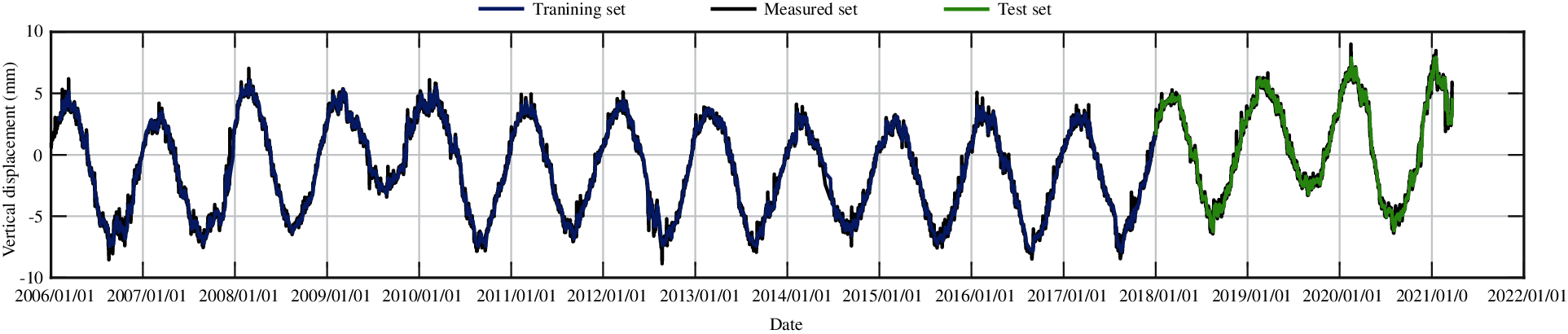
Figure 30: The training set and the test set of vertical displacement for measuring point J37 by LSTM method
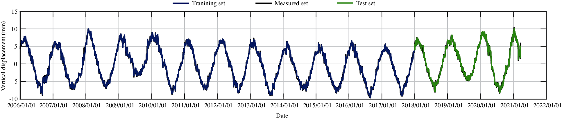
Figure 31: The training set and the test set of vertical displacement for measuring point J39 by LSTM method
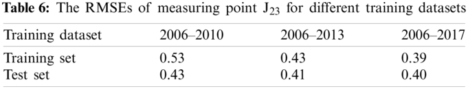
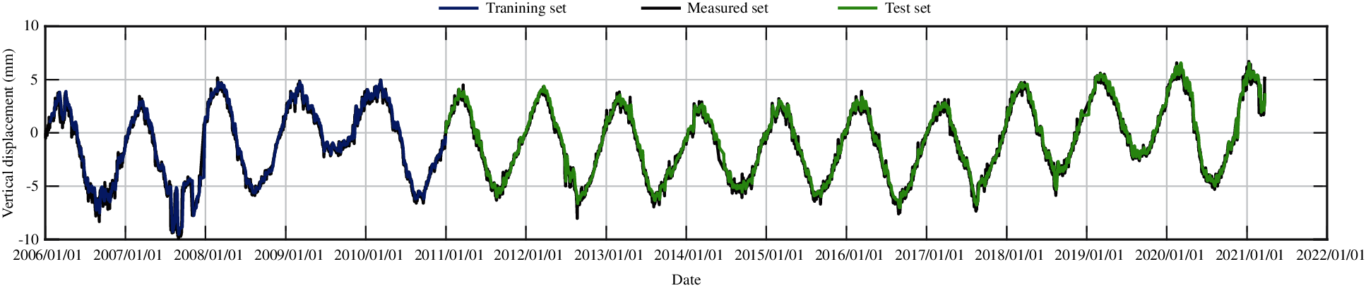
Figure 32: The training set and the test set of vertical displacement for measuring point J23 from the trained model (training dataset is from 2006 to 2010)
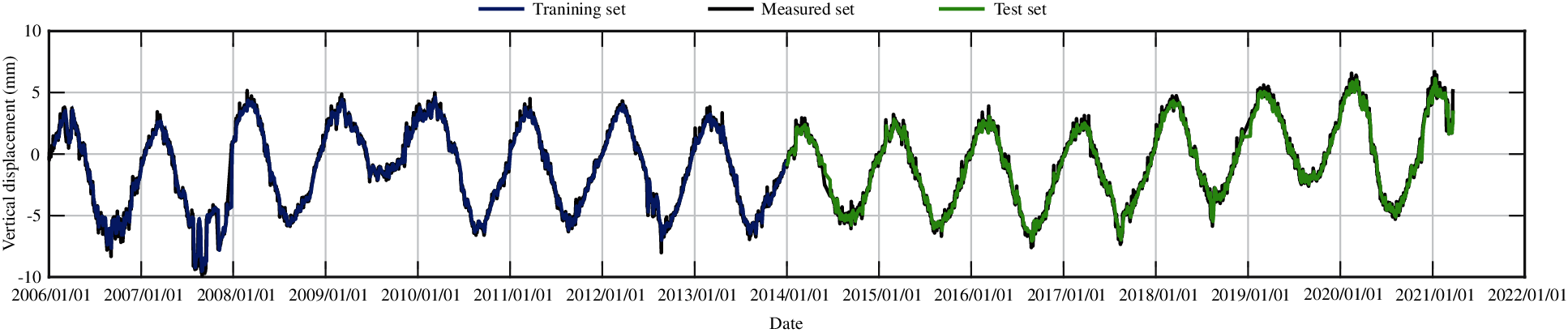
Figure 33: The training set and the test set of vertical displacement for measuring point J23 from the trained model (training dataset is from 2006 to 2013)
The fitting results of the stepwise regression model and partial least square regression model are very similar, and the model quality is good, which can reflect the subsidence change law of measuring points. The multiple correlation coefficient of the stepwise regression method is slightly bigger than that of the partial least square method, while the residual standard deviation of the stepwise regression method is much bigger than that of the partial least square method.
From the process lines of the stepwise regression model and the partial least square model, it is found that the temperature component changes most obviously, and the change of the water pressure component and aging component is small. In other words, the displacements of measuring points are greatly affected by temperature change and less affected by water level and aging. This can be found from the introduction sequence of independent variables of stepwise regression method, which is in accord with the actual situation of dam operation. The dam body rises or sinks when the temperature rises or drops, and the changes are periodic. This is consistent with the actual situation of the dam.
Because of the high linear correlation of factors in water pressure component, stepwise regression method removes the factors of primary term of upstream water level and primary and tertiary terms of downstream water level, which will affect the regression analysis accuracy to some extent. In this regard, the partial least square regression method is more advantageous.
In the aging component, the fitting of partial least square regression method shows that the dam has settlement effect, and the subsidence will gradually slow with the time. The fitting of stepwise regression method shows that the dam has the effect of rising, and the rising amount will decrease with the time. The measuring point is not the starting time of statistical model based on the time of dam construction, so the time component has displacement at the beginning. Generally speaking, the change law of aging displacement of normal operation dam is sharp change in the initial stage and tends to be stable in the later period. However, the real displacement curves of measuring points show that the measuring points have obvious subsidence trend, so the aging components of both models are not stable, which is in agreement with the actual situation. On the whole, the aging component obtained by the partial least square model is more fit for the real situation.
Fig. 34 presents the fitting results of vertical displacement for measuring point J23 obtained by the partial least squares model (PLS) and the stepwise regression model (STEPWISE) and the test results obtained by the LSTM model. From Fig. 34, in combination with Figs. 7, 17 and 27, it is found that the accuracy of the LSTM model is higher than those of the statistical models. However, the LSTM model cannot separate the influence of each component, in addition, the training data must be sufficient.
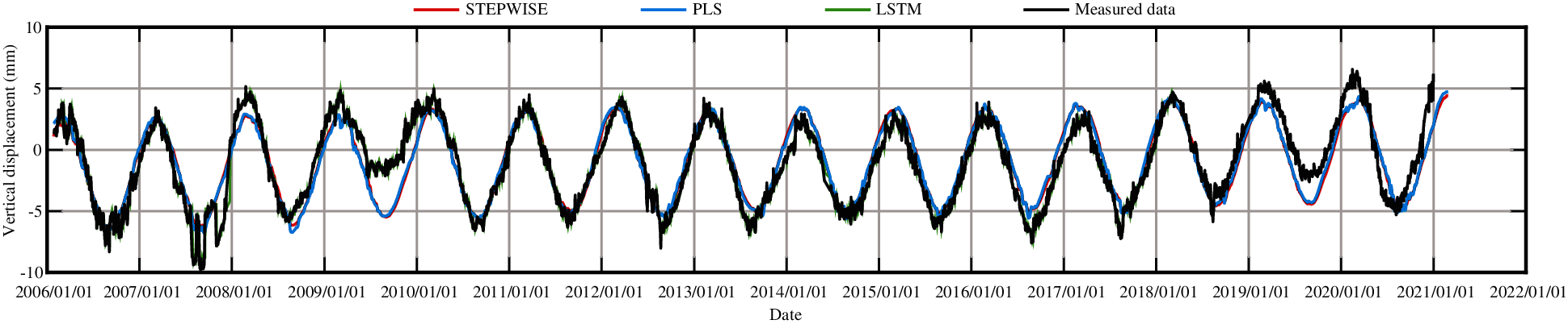
Figure 34: The prediction results of vertical displacement for measuring point J23 by different methods
Two statistical models and a deep learning model of vertical displacement at five typical measuring points located on the crest of Wuqiangxi dam are constructed by partial least square method, stepwise regression method and LSTM recurrent neural network. The fitting results and the influence of each component on displacement value in the statistical models are compared and analyzed, the test curve in the LSTM model is given and compared with the fitting curves of the statistical models. The following conclusions are drawn:
• The prediction accuracy of the LSTM model is higher than the statistical models when there are enough training data, so the LSTM model is suggested when there are enough training data.
• From the multiple correlation coefficient, the fitting results of partial least squares regression model and stepwise regression model are similar, and the residual standard deviation obtained by partial least squares regression model is lower.
• The stepwise regression model removes some factors, and has a large residual standard deviation. The partial least squares regression model considers factors comprehensively and explains each component more strictly.
• It is more appropriate to use partial least squares regression model or LSTM model to predict the subsidence of measuring points in Wuqiangxi dam.
In the deformation prediction of concrete gravity dam, the LSTM model is suggested when there are sufficient training data, and the partial least squares regression model is suggested when the training data are insufficient. In addition, all deformation, water level, and temperature data in this study can be accessed at: http://www.idmes.cn/data.html.
Acknowledgement: The authors wish to express their appreciation to the reviewers for their helpful suggestions which greatly improved the presentation of this paper.
Funding Statement: The authors received no specific funding for this study.
Conflicts of Interest: The authors declare that they have no conflicts of interest to report regarding the present study.
1. Hu, J., Ma, F. (2020). Statistical modelling for high arch dam deformation during the initial impoundment period. Structural Control and Health Monitoring, 27(12), e2638. DOI 10.1002/stc.2638. [Google Scholar] [CrossRef]
2. Yuan, D., Wei, B., Xie, B., Zhong, Z. (2020). Modified dam deformation monitoring model considering periodic component contained in residual sequence. Structural Control and Health Monitoring, 27(12), e2633. DOI 10.1002/stc.2633. [Google Scholar] [CrossRef]
3. Beaupré, L., St-Hilaire, A., Daigle, A., Bergeron, N. (2020). Comparison of a deterministic and statistical approach for the prediction of thermal indices in regulated and unregulated river reaches: Case study of the fourchue river (Quebec, Canada). Water Quality Research Journal of Canada, 55(4), 394–408. DOI 10.2166/wqrj.2020.001. [Google Scholar] [CrossRef]
4. Wei, B., Liu, B., Yuan, D., Mao, Y., Yao, S. (2021). Spatiotemporal hybrid model for concrete arch dam deformation monitoring considering chaotic effect of residual seriesn. Engineering Structures, 228, 111488. DOI 10.1016/j.engstruct.2020.111488. [Google Scholar] [CrossRef]
5. Pei, L., Wu, Z., Cui, M., Zhang, Q., Chen, J. (2012). Research and application on the displacement hybrid-model of high earth dam. Journal of Sichuan University (Engineering Science Edition), 44(Supl), 42–47. DOI 10.15961/j.jsuese.2012.s1.051. [Google Scholar] [CrossRef]
6. Zhen, D., Huo, Z., Li, B. (2011). Arch-dam crack deformation monitoring hybrid model based on XFEM. Science China Technological Sciences, 54(10), 2611–2617. DOI 10.1007/s11431-011-4550-6. [Google Scholar] [CrossRef]
7. Ren, Q., Li, M., Song, L., Liu, H. (2020). An optimized combination prediction model for concrete dam deformation considering quantitative evaluation and hysteresis correction. Advanced Engineering Informatics, 46, 101154. DOI 10.1016/j.aei.2020.101154. [Google Scholar] [CrossRef]
8. Wei, B., Yuan, D., Li, H., Xu, Z. (2019). Combination forecast model for concrete dam displacement considering residual correction. Structural Health Monitoring, 18(1), 232–244. DOI 10.1177/1475921717748608. [Google Scholar] [CrossRef]
9. Tatin, M., Briffaut, M., Dufour, F., Simon, A., Fabre, J. (2018). Statistical modelling of thermal displacements for concrete dams: Influence of water temperature profile and dam thickness profile. Engineering Structures, 165, 63–75. DOI 10.1016/j.engstruct.2018.03.010. [Google Scholar] [CrossRef]
10. Ding, J., Yu, T., Bui, T. (2020). Modeling strong/weak discontinuities by local mesh refinement variable-node XFEM with object-oriented implementation. Theoretical and Applied Fracture Mechanics, 106, 102434. DOI 10.1016/j.tafmec.2019.102434. [Google Scholar] [CrossRef]
11. Liu, G. (2009). Meshfree methods: Moving beyond the finite element method (Second Edition). USA: CRC Press. [Google Scholar]
12. Li, B., Yang, J., Hu, D. (2020). Dam monitoring data analysis methods: A literature review. Structural Control and Health Monitoring, 27, e2501. DOI 10.1002/stc.2501. [Google Scholar] [CrossRef]
13. Tonini, D. (1956). Observed behavior of several Italian arch dams. Journal of the Power Division, 82(6), 1–26. DOI 10.1061/JPWEAM.0000062. [Google Scholar] [CrossRef]
14. Wu, Z. (2003). Safety monitoring theory and its application of hydraulic structures (First Edition). Beijing: Higher Education Press. [Google Scholar]
15. Chen, J. (1980). The nonlinear parameter estimation of aging deformation of concrete dam. Dam Observation and Geotechnical Testing, (2), 3–13. DOI CNKI:SUN:DBGC.0.1980-02-000. [Google Scholar]
16. Léger, P., Leclerc, M. (2007). Hydrostatic, temperature, time-displacement model for concrete dams. Journal of Engineering Mechanics, 133(3), 267–277. DOI 10.1061/(ASCE)0733-9399(2007)133:3(267). [Google Scholar] [CrossRef]
17. Tatin, M., Briffaut, M., Dufour, F., Simon, A., Fabre, J. (2015). Thermal displacements of concrete dams: Accounting for water temperature in statistical models. Engineering Structures, 91, 26–39. DOI 10.1016/j.engstruct.2015.01.047. [Google Scholar] [CrossRef]
18. Mata, J., T. de Castro, A., Sá da Costa, J. (2014). Constructing statistical models for arch dam deformation. Structural Control and Health Monitoring, 21, 423–437. DOI 10.1002/stc.1575. [Google Scholar] [CrossRef]
19. Wang, S., Xu, C., Gu, C., Su, H., Hu, K. et al. (2020). Displacement monitoring model of concrete dams using the shape feature clustering-based temperature principal component factor. Structural Control and Health Monitoring, 27, e2603. DOI 10.1002/stc.2603. [Google Scholar] [CrossRef]
20. Hu, D., Zhou, Z., Li, Y., Wu, X. (2011). Dam safety analysis based on stepwise regression model. Advanced Materials Research, 204, 2158–2161. DOI 10.4028/www.scientific.net/AMR.204-210.2158. [Google Scholar] [CrossRef]
21. Shen, W., Ren, J. (2014). Multiple stepwise regression analysis crack open degree data in gravity dam. Applied Mechanics and Materials, 477, 888–891. DOI 10.4028/www.scientific.net/AMM.477-478.888. [Google Scholar] [CrossRef]
22. Chen, H., Sun, Y., Gao, J., Hu, Y., Yin, B. (2018). Solving partial least squares regression via manifold optimization approaches. IEEE Transactions on Neural Networks and Learning Systems, 30, 588–600. DOI 10.1109/TNNLS.2018.2844866. [Google Scholar] [CrossRef]
23. Cheng, X., Li, Q., Zhou, W., Zhou, Z. (2020). External deformation monitoring and improved partial least squares data analysis methods of high core rock-fill Dam (HCRFD). Sensors, 20(2), 444. DOI 10.3390/s20020444. [Google Scholar] [CrossRef]
24. Yin, W., Zhao, E., Gu, C., Huang, H., Yang, Y. (2019). A nonlinear method for component separation of Dam effect quantities using kernel partial least squares and pseudosamples. Advances in Civil Engineering, 2019, 1958173. DOI 10.1155/2019/1958173. [Google Scholar] [CrossRef]
25. Huang, H., Chen, B., Liu, C. (2015). Safety monitoring of a super-high Dam using optimal kernel partial least squares. Mathematical Problems in Engineering, 2015, 571594. DOI 10.1155/2015/571594. [Google Scholar] [CrossRef]
26. He, X., Leng, Y., Zhao, S. (2010). Threshold regression forecast model for dam safety monitoring and its application. Applied Mechanics and Materials, 36, 182–186. DOI 10.4028/www.scientific.net/AMM.36.182. [Google Scholar] [CrossRef]
27. Lan, S., Fang, C. (2012). Application of least square method based logistic regression model to settlement prediction of earth-rock fill dam. Water Resources and Hydropower Engineering, 43(3), 16–18. DOI 10.13928/j.cnki.wrahe.2012.03.011. [Google Scholar] [CrossRef]
28. Dai, B., Gu, C., Zhao, E., Qin, X. (2018). Statistical model optimized random forest regression model for concrete dam deformation monitoring. Structural Control and Health Monitoring, 25, 1–15. DOI 10.1002/stc.2170. [Google Scholar] [CrossRef]
29. Li, X., Wen, Z., Su, H. (2021). An approach using random forest intelligent algorithm to construct a monitoring model for dam safety. Engineering with Computers, 37, 39–56. DOI 10.1007/s00366-019-00806-0. [Google Scholar] [CrossRef]
30. Qu, X., Yang, J., Chang, M. (2019). A deep learning model for concrete dam deformation prediction based on RS-LSTM. Journal of Sensors, 2019, 4581672. DOI 10.1155/2019/4581672. [Google Scholar] [CrossRef]
31. Yang, D., Gu, C., Zhu, Y., Dai, B., Zhang, K. et al. (2020). A concrete dam deformation prediction method based on LSTM with attention mechanism. IEEE Access, 8, 185177–185186. DOI 10.1109/Access.6287639. [Google Scholar] [CrossRef]
32. Liu, W., Pan, J., Ren, Y., Wu, Z., Wang, J. (2020). Coupling prediction model for long-term displacements of arch dams based on long short-term memory network. Structural Control and Health Monitoring, 27, e2548. DOI 10.1002/stc.2548. [Google Scholar] [CrossRef]
33. Han, B., Geng, F., Dai, S., Gan, G., Liu, S. et al. (2020). Statistically optimized back-propagation neural-network model and Its application for deformation monitoring and prediction of concrete-face rockfill dams. Journal of Performance of Constructed Facilities, 34(4), 04020071. DOI 10.1061/(ASCE)CF.1943-5509.0001485. [Google Scholar] [CrossRef]
34. Chen, S., Gu, C., Lin, C., Hariri-Ardebili, M. (2021). Prediction of arch dam deformation via correlated multi-target stacking. Applied Mathematical Modelling, 91, 1175–1193. DOI 10.1016/j.apm.2020.10.028. [Google Scholar] [CrossRef]
35. Shi, Z., Gu, C., Zhao, E., Xu, B. (2020). A novel seepage safety monitoring model of CFRD with slab cracks using monitoring data. Mathematical Problems in Engineering, 2020, 1641747. DOI 10.1155/2020/1641747. [Google Scholar] [CrossRef]
36. Yang, J., Qu, X., Chang, M. (2019). An intelligent singular value diagnostic method for concrete dam deformation monitoring. Water Science and Engineering, 12(3), 205–212. DOI 10.1016/j.wse.2019.09.006. [Google Scholar] [CrossRef]
37. Liu, X., Kang, F., Ma, C., Li, H. (2021). Concrete arch dam behavior prediction using kernel-extreme learning machines considering thermal effect. Journal of Civil Structural Health Monitoring, 11, 283–299. DOI 10.1007/s13349-020-00452-x. [Google Scholar] [CrossRef]
38. Chen, S., Gu, C., Lin, C., Zhang, K., Zhu, Y. (2021). Multi-kernel optimized relevance vector machine for probabilistic prediction of concrete dam displacement. Engineering with Computers, 37, 1943–1959. DOI 10.1007/s00366-019-00924-9. [Google Scholar] [CrossRef]
39. Shu, X., Bao, T., Li, Y., Gong, J., Zhang, K. (2021). VAE-Talstm: A temporal attention and variational autoencoder-based long short-term memory framework for dam displacement prediction. Engineering with Computers, DOI 10.1007/s00366–021–01362–2. [Google Scholar] [CrossRef]
40. Chen, W., Wang, X., Cai, Z., Liu, C., Zhu, Y. et al. (2021). DP-Gmm clustering-based ensemble learning prediction methodology for dam deformation considering spatiotemporal differentiation. Knowledge-Based Systems, 222, 106964. DOI 10.1016/j.knosys.2021.106964. [Google Scholar] [CrossRef]
 | This work is licensed under a Creative Commons Attribution 4.0 International License, which permits unrestricted use, distribution, and reproduction in any medium, provided the original work is properly cited. |