Computer Modeling in Engineering & Sciences

DOI: 10.32604/cmes.2022.018339

ARTICLE

Remote Sensing Image Retrieval Based on 3D-Local Ternary Pattern (LTP) Features and Non-subsampled Shearlet Transform (NSST) Domain Statistical Features

Hilly Gohain Baruah*, Vijay Kumar Nath and Deepika Hazarika

Department of Electronics and Communication Engineering, Tezpur University, Assam, 784028, India
*Corresponding Author: Hilly Gohain Baruah. Email: hilly90@tezu.ernet.in
Received: 17 July 2021; Accepted: 22 October 2021

1  Introduction

Due to advances in remote imaging sensors and earth observation technologies, the volume of high resolution remote sensing images have increased dramatically. Urbanization preparation, deforestation detection, weather prediction, farm monitoring, and military applications are only a few of the uses for remote sensing images. Hence, precise image retrieval techniques for remote sensing images are very important [1–4]. The increase in spatial resolution and database volume have led to difficulties in the manual annotation based image retrieval approaches. Hence it is very important to have a proper management framework to deal with this huge volume of remote sensing data. Image retrieval techniques based on image content plays crucial role to handle this data properly. Feature extraction and similarity measurement are the two key modules in content based image retrieval (CBIR). In the feature extraction module, features that describe visual content of an image are extracted, and then the similarity between the features extracted from the query and the database images is calculated. Remote sensing images consist of semantic objects of wide range as they cover quite large geographical area. The main challenge in case of remote sensing images is the presence of variations in appearance in semantic objects of same category [2]. Hence for retrieval of remote sensing images, the features extracted should be highly robust and descriptive. The time requirement for retrieval of images of interest out of the huge volume of remote sensing data is also to be considered while designing an efficient remote sensing image retrieval framework.

The texture, color and shape information are the primary visual attributes of any high resolution remote sensing images and describes important details for scene retrieval. The most of the earlier literature are based on these features. The various handcrafted features like scale invariant feature transform (SIFT) [5], color histogram [6], gist [7], histogram of oriented gradients (HOG) [8] and local binary pattern (LBP) [9], etc. exist in the literature. The color histogram and gist describes the global features whereas the SIFT, HOG and LBP describes the local features of an image. Global features denote the visual details of an image as a whole. The macrostructure informations in an image can be well captured with global features. In [1], Ferecatu and Boujemaa for image retrieval employed global image descriptors that are constructed using statistical representation of color, texture as well as shape features and demonstrated few search examples that exhibits the effectiveness of relevance feedback on remote sensing images. In [10], Ma et al. proposed a shape based descriptor that uses region and polygonal extraction. In an another approach, Yang et al. [11] showed the use of color layer based texture elements histogram along with color fuzzy correlogram for retrieval of remote sensing images. Few techniques employ both statistical model and multiresolution analysis to describe the global features of the images. Choy et al. [12] modeled the wavelet coefficients of images using three parameter generalized Gamma distribution and used its parameters to describe the texture feature. In [13], the image wavelet subband coefficients were modeled using finite mixtures of generalized Gaussian distribution. The parameters of this distribution were used as features to describe the subband images. Liu et al. [14] modeled the NSST coefficients of remote sensing images using Bessel K distribution and used its parameters to describe the texture feature. In [3], another remote sensing image retrieval approach based on statistical modeling was introduced where the symmetric normal inverse Gaussian (SNIG) distribution was used to model detail subbands of the NSST. The estimated SNIG parameters were used to construct the feature vector. The main strength of transform domain statistical modeling based techniques is that the texture discrimination here is treated as an issue of similarity measurement between statistical distributions, which is relatively easy to implement when compared to Markov random fields [15]. The global feature based techniques are usually effective on the categories that are largely texture based and carries image-scale details. The local feature based techniques however are effective in the categories which exhibits definite or perceptible structures whose presence/absence is used to discriminate the images. The local pattern based schemes such as LBP [16], local ternary pattern (LTP) [17], etc. captures microstructure information only and is highly appropriate for dense local feature extraction. In [18,19], a technique using patch based complete local binary pattern in multi-scale framework is introduced for remote sensing image scene classification. Bian et al. introduced extended multi-structure local binary pattern for scene classification of remote sensing images. In [20], the original Bag-of-words (BOW) model was improved by characterizing the images using local features that are extracted from base images for retrieval of remote sensing images. Sukhia et al. [21] proposed to use LTP in three different scales for extraction of features from remote sensing images. These features are then encoded with Fisher vector encoding scheme.

Both global and local features capture complementary informations and their combinations are observed to be effective in improving the retrieval and classification performance. In order to describe a high resolution image scene with high diversity, many techniques fail to supply discriminative details especially when some major structural information in the image usually dominate the image class. In such cases, the fusion of both local and global features are usually preferred to obtain improved performance [22,23]. In the last one decade, various schemes [24–31] have been introduced that combine both local and global features. In [24], Bian et al. fused the local features that are extracted using codebookless model and the global features that are exploited using saliency based multiscale multiresolution multistructure local binary pattern for classification of high resolution remote sensing scenes. In [25], Risojevic et al. extracted local features employing the SIFT and global features utilizing the enhanced Gabor texture descriptor, and were combined using a scheme to enhance the classification of remote sensing image scenes. In [26], Liu et al. introduced median robust extended LBP (MRELBP) which not only captures microstructure information but macrostructure too. In [27], Yang et al. extracted global features from high pass subband images of dual-tree complex wavelet and local features from LBP applied on all low pass subband images. The authors finally combined both these features for texture classification. In [28], Kabbai et al. combined both local and global features for image classification. Local features were extracted using speeded up robust feature descriptor and the global features were extracted through combination of wavelet transform based features with modified form of local ternary pattern (LTP). A multiple feature based regularized kernel is introduced for classification of hyperspectral images [29]. Various spatial features such as local feature, shape, spectral and global features are combined to supply more discriminative information. For local, global and shape features; LBP feature, Gabor feature and extended multiattribute profiles are exploited respectively.

It is discussed in [14] that the combination of features not everytime assures improved retrieval performance. For any images with high amount of details, it is essential to select efficient features that are supportive to each other in order to achieve improved retrieval results and to effectively blend them without increase in feature dimensions. Motivated from [3,14,24,27], we introduce a remote sensing image retrieval technique that uses an effective combination of new local 3D-LTP based features and novel global NSST domain statistical features. The 3D-LTP descriptor encodes both the colour cue information and local texture details. It is shown that the 2-state LM distribution best fits the statistics of detail NSST subband coefficients than BKF, Laplacian and SNIG distributions. Through accurate statistical modelling we calculate the discriminative global texture features from NSST subbands using the 2-state LM distribution parameters along with subband kurtosis and skewness. Since the local or global features describes complementary image informations and alone cannot provide discriminative description in many situations, we propose an effective blend of global and local features along with colour information to improve the discriminativeness of the features. The proposed NSSTds-3DLTP outperforms Gabor RGB, Granulometry, LBP, FV, VLAD and MRELBP descriptors in terms of MAP, ANMRR and P-R curve analysis for WHU-RS19,AID and PatternNet datasets. The NSSTds-3DLTP is highly suitable in retrieval of high resolution remote sensing images where accurate and fast search procedures are required in order to retrieve the most relevant images.

The main contributions of the paper are:

1.    The image NSST detail subband coefficients are modeled using 2-state Laplacian mixture model. It is demonstrated that the 2-state Laplacian mixture model best fits the subband coefficients when compared to other highly non-Gaussian distributions such as Laplacian, Bessel K form and SNIG. The 2-state Laplacian mixture model parameters in addition with kurtosis and skewness are calculated from detail subbands, and the mean along with standard deviation are calculated from the approximation subband and are concatenated together to construct the feature vector, to represent the global features of the image. This global feature is referred to as NSSTds.

2.    Since the classical LTP ignores the encoding of color feature which is also one of the crucial visual attribute, an extension to 3D-LTP is introduced in this paper in order to encode not only the local intensity variations across the planes but also the color information.

3.    The proposed fusion of local and global features achieves highly discriminative feature representation with much less dimensions. This feature fusion is referred to as NSSTds-3DLTP.

The paper is organized with the following structure. Section 2 presents a brief review on NSST and detailed description on proposed framework in remote sensing image retrieval. Section 3 reflects the performance analysis on the experimental outcomes obtained. Section 4 concludes the paper.

2  Methodology

2.1 Nonsubsampled Shearlet Transform (NSST)

Though wavelet transform deals effectively with the point singularities of signals, it fails to capture the linear singularities that exist in the images [32]. To handle this problem, different multi-geometric analysis tools such as curvelet [33], contourlet [34] and shearlet transform [35] were introduced in the literature.

NSST inherits the benefits of classic theory of the affine systems, i.e., it is an extension of the wavelet theory. The important properties of NSST such as localiztion, multiscale, translational invariance and high directional sensitivity enables the NSST to provide a powerful image representation. Inspite of the significant developments that has been made, the effective texture description is still a demanding problem that needs attention. Therefore, in this paper we intend to develop a shearlet based texture descriptor to describe the texture information more effectively.

The continuous shearlet transform (ST) of image f in two dimension can be defined as follows:

STφ,f(i,s,t)=<f,φi,s,t> (1)

where i, t and s represents scale, translation and orientation parameters, respectively [32]. The shearlet function φ(i,s,t) is defined as

φi,s,t=|detKi,s|−1/2φ(Ki,s−1(a−t));i>0,s∈R,t∈R2,φ∈L2(R2) (2)

The notation L2 denotes a vector space of square integrable functions on a 2-D euclidean space R2.

The parameter Ki,s=[i−is0i] for i>0, s∈R, t∈R2. The Ki, s matrix can be factorized as Ki,s=[1−s01][i00i]=BsAi where Bs and Ai denotes shear and diagonal matrices. It is important to note that anisotropic dilation is carried out by Ai (for multiscale partitions) and shearing is done by Bs matrix (for directional analysis).

In NSST, nonsubsampled Laplacian pyramid (NSLP) filtering results in low and high frequency components and directional filtering with different shearing matrices lead to shift invariant form of shearlet transform. The NSST removes the up sampling and down sampling operations unlike shearlet transform and therefore is completely invariant [36,37]. Also NSST is multi-scale and has got high directional selectivity. Therefore the use of NSST in image retrieval applications could do justice to these powerful features of NSST in effectively describing the features of input image.

In Fig. 1, a visual example of image NSST approximation and detail subbands for one remote sensing image is shown. The NSST approximation and detail subbands (Fig. 1) refer to the subbands that contains low-frequency coefficients and the high-frequency coefficients respectively. Figs. 1d–1e and 1f–1i respectively shows high frequency detail coefficients at the finest scale/Scale 1 and at next coarsest scale, i.e., Scale 2.

2.2 The Proposed Remote Sensing Image Retrieval Framework

This subsection describes the proposed NSSTds-3DLTP feature in a RSIR framework in details. The framework consists of two major modules. The first module calculates the global NSSTds features using NSST-domain statistical parameters and the second module calculates the local 3D-LTP features from RGB channels. The proposed global NSSTds features are combined with proposed local 3D-LTP features to generate a fused representation NSSTds-3DLTP leading to an enhanced feature description.

The block diagram of NSSTds-3DLTP based framework is presented in Fig. 2.

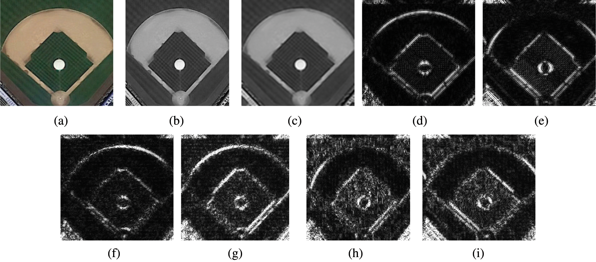
Figure 1: Example of NSST 2-level decomposition of a remote sensing image from PatternNet dataset. (a) Original image; (b) Its grayscale form; (c) Approximation subband; (d) 1st Detail subband (Scale 1); (e) 2nd Detail subband (Scale 1); (f) 1st Detail subband (Scale 2); (g) 2nd Detail subband (Scale 2); (h) 3rd Detail subband (Scale 2); (i) 4th Detail subband (Scale 2)

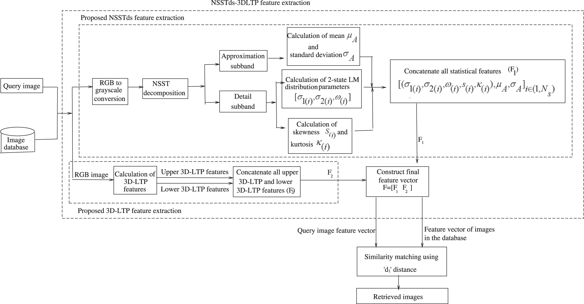
Figure 2: The block diagram of proposed NSSTds-3DLTP descriptor in an image retrieval framework

2.2.1 Computation of NSST Domain Statistical Features (NSSTds)

With statistical modeling of transform coefficients, the texture discrimination problem can be solved with much less dimensions by simply measuring the similarity between the statistical models. This technique is relatively easier to implement and is highly effective. The parametric distributions have been employed to model the image transform coefficients distribution, for retrieval of images [3,14]. In the literature, wavelet transform domain statistical modeling of images have been quite popular. The non-Gaussian distributions such as generalized Gaussian, finite mixture of generalized Gaussian [13] and generalized Gamma [12] based models have been successfully used in image retrieval applications. The discrete wavelet transform are not capable of describing the linear singularities present in images. As also discussed in previous subsection, the multiscale geometric analysis tools such as shearlet provides solution to the above problem as this transform provides excellent sparse representation for higher dimensional singularities. Very recently in [3], it was demonstrated that the image NSST coefficients obey highly non-Gaussian statistics and the symmetric normal inverse Gaussian (SNIG) distribution was shown to be more appropriate than Laplacian and BKF models [14] in modeling the NSST detail coefficients of remote sensing images. Laplacian mixture (LM) model has been known for its good ability to capture very heavy tails of highly non-Gaussian empirical data. It should be noted that the tails of mixture of two Laplacian distributions decays slower than the tail of one Laplacian distribution. The mixture of three or more Laplacian distributions may give more heavy tails than a single Laplacian distribution or mixture of two Laplacian distributions, however as the number of parameters to be estimated increases the potential to estimate them accurately gets decreased. Therefore, we propose to model the NSST subband coefficients of remote sensing images using 2-state LM model [38,39].

In this paper, a mixture of two individual Laplacian distributions is referred to as 2-state LM distribution or model. Let Px(j)(x(j)) (where j=1,2…NT and NT is the no. of set of coefficients) denote a 2-state LM model for modeling the image NSST high-frequency detail coefficients x(j) which is expressed as [38]:

Px(j)(x(j))=ω(j)P1(x(j))+(1−ω(j))P2(x(j)) (3)

where ω(j) and (1−ω(j)) are the weights to two individual Laplacian pdf’s P1(x(j)) and P2(x(j)), respectively.

When P1(x(j))=1σ1(j)2e−2|x(j)|σ1(j) and P2(x(j))=1σ2(j)2e−2|x(j)|σ2(j), Eq. (3) can be expressed as:

Px(j)(x(j))=ω(j)1σ1(j)2e−2|x(j)|σ1(j)+(1−ω(j))1σ2(j)2e−2|x(j)|σ2(j) (4)

The σ1(j) and σ2(j) respectively are the standard deviations of individual pdf’s P1(x(j)) and P2(x(j)). The parameters σ1(j), σ2(j) and ω(j) are first initialized and then estimated using Expectation-Maximization (EM) algorithm [38,39].

To estimate the parameters of 2-state LM distribution, the parameters [σ1,σ2,ω] are first initialized and subsequently the Expectation Maximization computation procedures are iteratively carried out till the condition of convergence is reached.

Expectation procedure: In this procedure, for each iteration the responsibility element r1(j) is calculated using:

r1(j)←ω(j)P1(x(j))ω(j)P1(x(j))+(1−ω(j))P2(x(j)) (5)

and

r2(j)←(1−r1(j)) (6)

The responsibility elements must assure r1(j)+r2(j) = 1 .

Maximization procedure: The ω(j) is calculated using:

ω(j)←1Nm∑i∈Nm(j)r1(i) (7)

where Nm(j) denotes a square shaped local window with Nm coefficients inside it and is positioned at the x(j) as center. The σ1(j) and σ2(j) are calculated using:

σ12(j)=∑i∈Nm(j)r1(i)|x(j)|2∑i∈Nm(j)r1(i) (8)

σ22(j)=∑i∈Nm(j)r2(i)|x(j)|2∑i∈Nm(j)r2(i) (9)

In order to defend the use of 2-state LM model in modeling the statistics of NSST coefficients, we perform Kolomogrov-Smirnov (KS) goodness of fit test [38] considering Laplacian, BKF and SNIG as probable models. The KS test statistic supplies the information on distance between empirical CDF (ECDF) and the CDF of a probable distribution. In this test, while calculating the distance information between ECDF and each probable distributions CDF, the one which give minimum KS statistic value is declared as the best fit for the given empirical data.

Mathematically, the KS test can be expressed as [38]:

KSv=maxx∈N|F(x)−F^(x)| (10)

where F^(x) and F(x) are the ECDF and CDF of the model respectively. The parameter x in Eq. (10) denotes the emprical data, i.e., the high frequency NSST detail coefficients whereas N denotes the total number of coefficients in the set of data.

Table 1 exhibits the average KS test statistics for remote sensing images taken from well known WHU-RS19 image dataset.

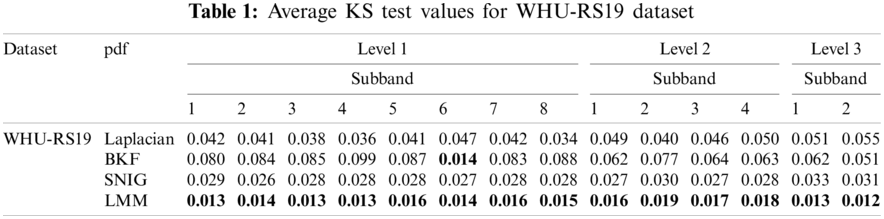
For the purpose of performing KS test, we consider a 3-level NSST decomposition (with 1,2,3 directions) that yields one approximation subband and a total of 14 detail subbands. The KS test was performed on 20 random images taken from diverse classes such as ‘Airport’, ‘Beach’, ‘bridge’, ‘commercial’, ‘desert’, ’farmland’, ‘footballfield’, ‘forest’, ‘Industrial, ‘Meadow’, ‘Park’, ‘River’, ‘Pond’, ‘Railway’, ‘Port’ and ‘Residential’ of WHU-RS19 dataset and finally averaged in order to find the most appropriate distribution that approximates the statistics of high-frequency NSST detail coefficients, considering Laplacian, BKF and SNIG distributions. It is clearly visible from Table 1 that for most of the subbands, the KS test value for 2-state LM model is the smallest that reveals clearly that it is able to approximate the detail subband coefficients better than Laplacian, Bessel K form (BKF) and SNIG distributions.

In addition to KS test and to further demonstrate the suitability of 2-state LM distribution in modeling the image NSST detail coefficients, we plotted the histogram plots (Fig. 3) of various detail subbands of NSST in logarithmic domain where Laplacian, BKF, SNIG and LM model pdf’s are fitted in log domain. Fig. 3 clearly demonstrates the superiority of 2-state LM distribution in approximating the statistics of high frequency detail coefficients as compared to other statistical models. Both Fig. 3 (through log histogram plots) and Table 1 (through KS test statistic) confirms that the 2-state LM model provides best fit compared to Laplacian, BKF and SNIG distributions.

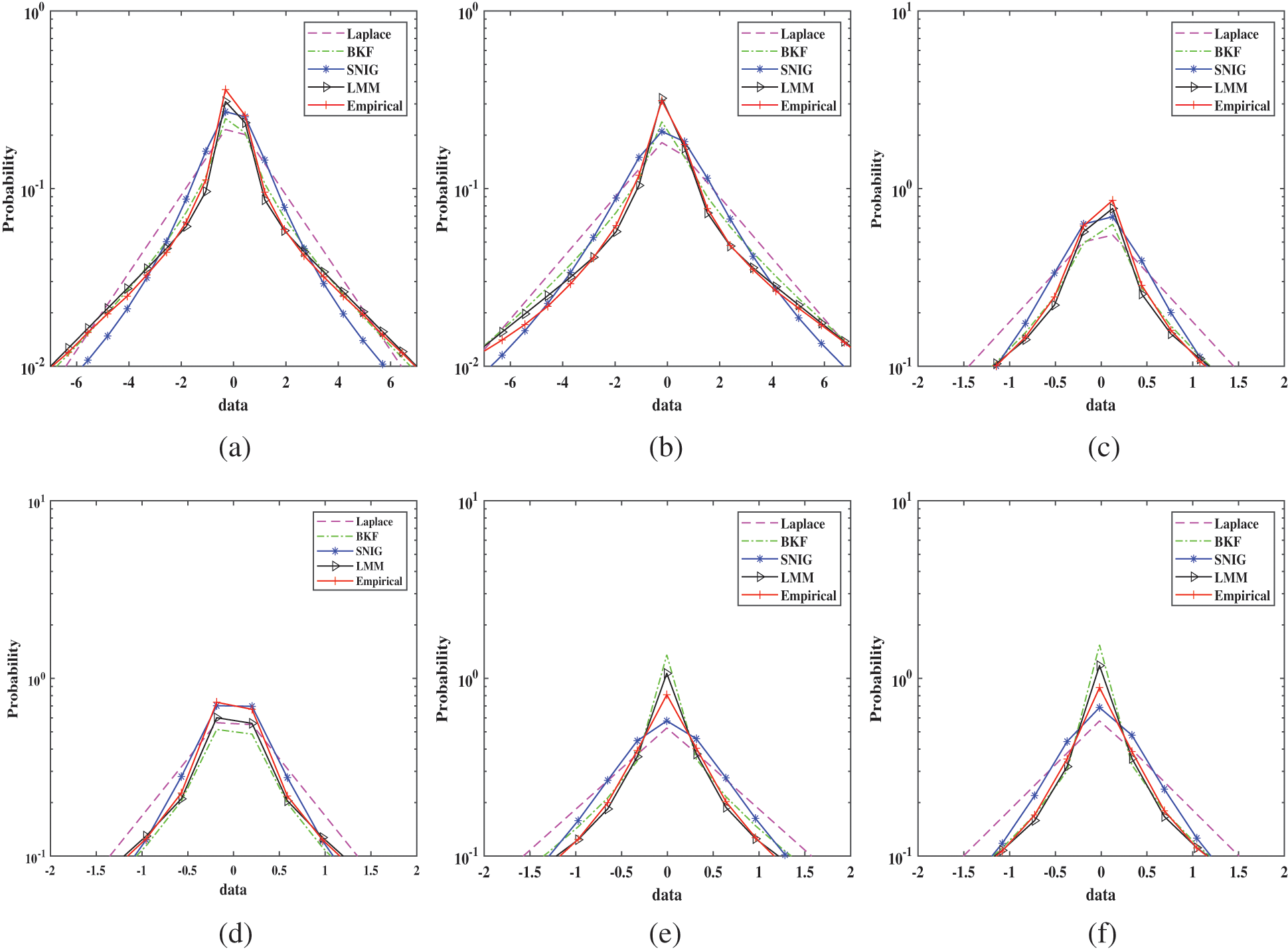
Figure 3: The log histogram plot for six NSST subbands of one example image from WHU-RS19 dataset where Laplacian, BKF, SNIG and LM pdfs are fitted to empirical histogram in log domain. (a) Subband 1 (Scale 1); (b) Subband 2 (Scale 1); (c) Subband 1 (Scale 2); (d) Subband 2 (Scale 2); (e) Subband 3 (Scale 2); (f) Subband 4 (Scale 2)

Given the 2-state LM model, the probability density function (pdf) of NSST coefficients in each subband can be fully described using three parameters σ1,σ2,ω. We use two more statistical parameters namely skewness (s) and kurtosis (κ) to describe the detail NSST subband coefficients. The skewness and kurtosis indicates about the distribution symmetry and distribution peakedness respectively. For a given sample of n values, we calculate the sample kurtosis and skewness using following expressions:

s=1n∑i=1n(xi−x¯)3[1n∑i=1n(xi−x¯)2]3/2 (11)

κ=1n∑i=1n(xi−x¯)4[1n∑i=1n(xi−x¯)2]2 (12)

where xi and x¯ denotes the ith value of x and the sample mean, respectively.

We use simple statistical mean and standard deviation features to describe the statistics of approximation subband.

σ=1n∑i=1n(xi−x¯)2 (13)

μ=1n(∑i=1nxi) (14)

Finally to describe the image NSST subbands using statistical features, we calculate the 2-state LM distribution parameters (σ1,σ2,ω), skewness (s) and kurtosis (κ) from each detail subband along with the mean (μA) and standard deviation σA estimated from the approximation subband, and concatenate them to construct the NSSTds feature vector as: F1=[(σ1(i),σ2(i),ω(i),s(i),κ(i)),μA,σA]i∈(1,Ns) (Ns is the total number of detail subbands).

2.2.2 Computation of Inter-Channel 3D-Local Ternary Pattern (3D-LTP) Features

The NSSTds proposed in previous subsection are regarded as global features of an image. The global feature based description however fails to describe the detailed arrangement and perceptible objects present in an image which usually can be best described using local features. For instance, few land use and land cover based categories are illustrated largely by discrete objects such as baseball fields and storage tanks. In order to address this issue we propose a new 3D-LTP based technique where it is directly applied on the spatial RGB color channels [40].

The 2-fold motivation of extension of LTP to 3D-LTP are:

1.    Since the RGB planes have high inter-plane correlation, the 3D-LTP exploits the relationship between a pixel intensity in one plane with respect to the neighbors in the next plane in reference to the same spatial position, thus capturing the color cue information too.

2.    Since the 3D-LTP can capture the above local inter-plane relationship, the process behaves like a high-pass kind of filter which catches the local intensity variations in an orientation.

The traditional and popular LBP technique [9] describes the texture feature by computing a LBP value where a center pixel is compared to all its neighbors in a circular neighborhood and a 0/1 is assigned to each neighbor based on the center pixel and neighboring pixel difference as follows:

LBPR,T=∑i=1T2i−1f(I(pi)−I(pc)) (15)

f(x)={1x≥00else (16)

where I(pc) is the center pixel value, I(pi) are the neighboring values, T denotes the total no. of neighbors and R is the neighborhood radius.

Tan and Triggs proposed a 3-valued code called local ternary pattern (LTP) [17] which is an extension to LBP where the pixel values in the range of ± threshold (th) around I(pc) are quantized to 0, for the values above (I(pc)+th) are quantized to +1 and the values less than (I(pc) − th) are quantized to −1. The function f(x) is thus modified as follows:

f(x,I(pc),th)={+1x≥I(pc)+th0|x−I(pc)|<th−1x≤I(pc)−th (17)

where x = (I(pi) − I(pc)). A sample example of LBP and LTP calculation is shown in Fig. 4.

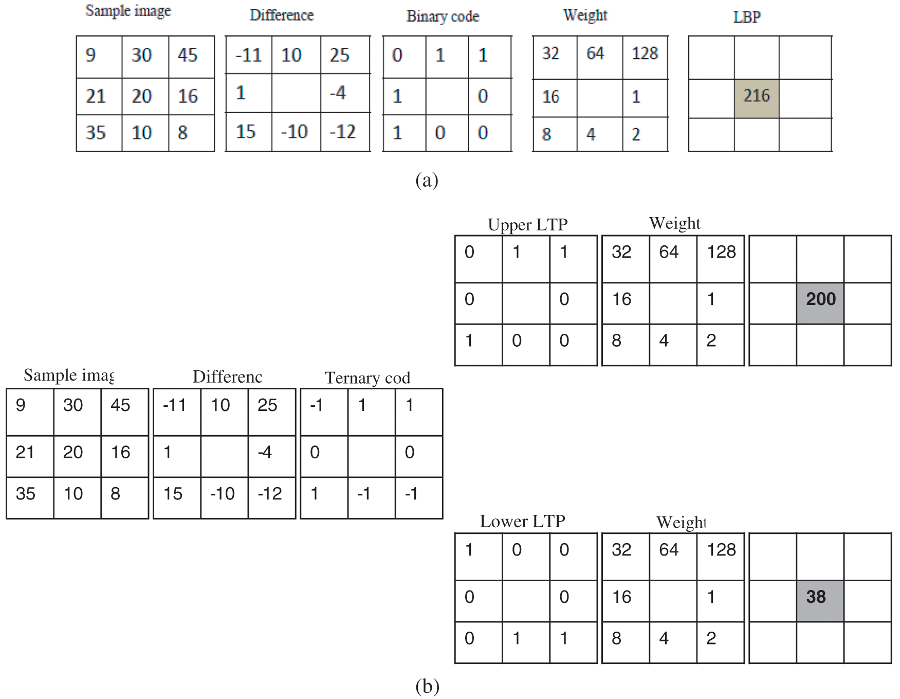
Figure 4: Example of LBP and LTP calculation for a sample image. (a) LBP; (b) LTP (for threshold 5)

LTP can capture image details better than LBP, as LTP provides 3 valued code to the difference between centre pixel and its neighbouring pixels.

The extension to 3D-LTP encodes not only the color cue information but also the local texture information in a color image. Given a RGB color image, the proposed inter-channel 3D-LTP produces six new images as shown in sample example computation in Fig. 5. The encoding of R channel considers the center/reference pixel in R and consider neighbors from G channel. Similarly, the encoding of G channel considers center/reference pixel in G channel and neighbors from B channel and the center/reference pixel in B channel consider neighbors from R channel for encoding B channel. The pattern images formed with 3D-LTP are presented in Fig. 6. Inter channel LTP when calculated for each of R-G, G-B and B-R combination provides one upper and one lower LTP. Therefore the R-G, G-B and B-R combinations produces a total of six pattern images, i.e., three upper LTPs and three lower LTPs.

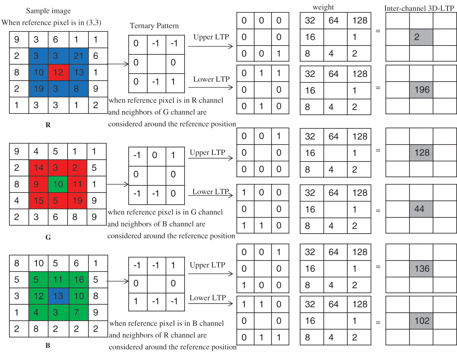
Figure 5: A sample example for 3D-LTP calculation

To reduce the feature dimensions, we identify and consider only the ‘uniform’ patterns in 3D-LTP. In this paper, the ‘uniform’ refers to uniform appearance of 3D local ternary patterns which means the patterns that have two or less number of discontinuities in circular binary representation and rest are referred to as non-‘uniform’ [16]. For example, 000100002 is an uniform pattern as it has only 2 bitwise 0/1 transitions and 00101001 is non-‘uniform’ pattern with more than 2 spatial transitions. It is observed that these ‘uniform’ patterns constitutes a majority of patterns that corresponds to important features like edges, textures, sharp corners, etc. For an image with R=1 and T=8, the unique ‘uniform’ patterns would be 58.

2.2.3 Fusion of NSST-Domain Statistical Features (NSSTds) and 3D-LTP Based Features

For describing a complex scene having complicated patterns and spatial structures, the blend of complementary features such as local and global features are usually preferred to achieve good results. In this subsection, we introduce a fused feature description using NSSTds and 3D-LTP based features for retrieval of remote sensing images.

If feature vector F1=[(σp1(i),σp2(i),ω(i),s(i),κ(i)),μA,σA]i∈(1,Ns) denotes the NSSTds calculated from detail and approximation subbands and F2 is the feature vector obtained from 3D-LTP ‘uniform’ histograms, then the final feature vector is described by F = [F1, F2].

For example, if an input image is decomposed using 4-level NSST with 3,3,4,4 directions (coarser to finest scale), we obtain a total of 49 subbands. Among these 49 subbands, one is low-frequency approximation subband and rest 48 are high-frequency detail subbands, i.e., 8(23), 8(23), 16(24) and 16(24) exists in Scale 4 (most coarsest), Scale 3, Scale 2 and Scale 1 (finest) respectively. With NSSTds, each high-frequency detail subband is represented by a 5 dimensional feature vector, so a total of 48 detail subbands will provide a feature vector of dimension (48×5)=240. Since only standard deviation and mean parameters are used to describe an approximation subband, a total of (240+2) = 242 dimension is required by NSSTds descriptor to describe a total of 49 subbands (both approx.+detail subbands). From Fig. 5 it can be clearly seen that with 3D-LTP technique (using uniform features), a total of 6, i.e., 3 upper LTP and 3 lower LTP feature maps are obtained. As 59 uniform features are obtained as a result of encoding a single feature map, a total of (59×6)=354 features are therefore required to Encode 6, i.e., 3 upper and 3 lower LTP feature maps. For the given NSST decomposition setting, finally with proposed NSSTds-3DLTP a total of 242+354 = 596 features are obtained.

2.2.4 Steps of NSSTds-3DLTP Feature Extraction Methodology

The algorithm for the proposed feature extraction technique is as follows:

Input-Image; Output-Feature vector

1.    Convert the color remote sensing image into gray scale image.

2.    Apply the NSST on the gray scale image.

3.    Extract the 2-state LMM parameters, kurtosis and skewness from each NSST detail subband and concatenate it with the mean (μA) and standard deviation (σA) calculated from the approximation subband to form the feature vector F1.

4.    Calculate the 3D-LTP based features from the R,G,B color channels of original remote sensing image to form the feature vector F2.

5.    The NSST-domain statistical features (NSSTds) and the 3D-LTP based features are finally concatenated to form the final feature vector set F = [F1, F2] after normalization.

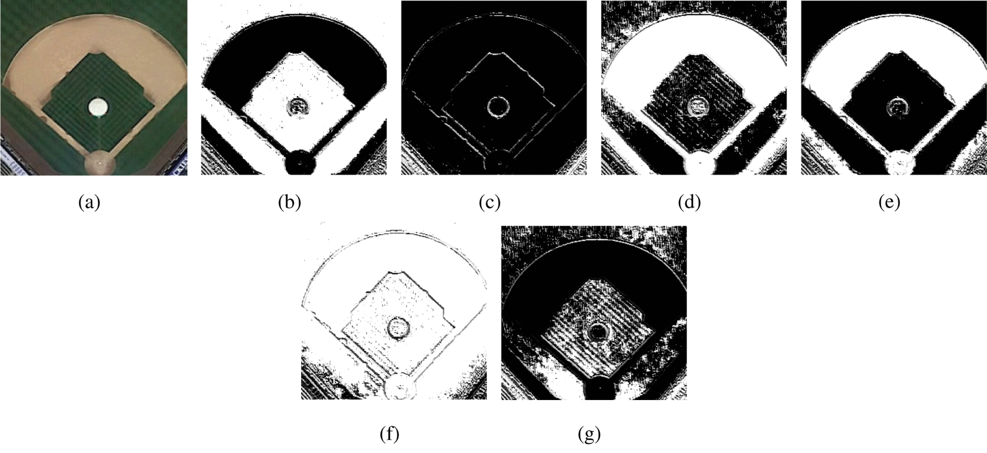
Figure 6: The pattern images obtained for an image from PatternNet dataset with inter channel 3D-LTP (a) Original image (b) Upper LTP pattern image after encoding R channel, (c) Lower LTP pattern image after encoding R channel, (d) Upper LTP pattern image after encoding G channel, (e) Lower LTP pattern image after encoding G channel, (f) Upper LTP pattern image after encoding B channel, (g) Lower LTP pattern image after encoding B channel

2.2.5 Similarity Measure

The extracted features of query image and database images are matched using a similarity metric. In the experiments, the NSSTds-3DLTP features has been evaluated using ‘d1’, Euclidean, Manhattan, Canberra and Chi-square similarity measures.

It has been observed that NSSTds-3DLTP exhibits best retrieval performance with ‘d1’ distance measure in comparison to Euclidean, Manhattan, Canberra and Chi-square distance measures. Therefore, the NSSTds-3DLTP descriptor employs ‘d1’ distance measure for feature matching in the image retrieval framework.

The d1 distance measure is given by:

D(dk,q)=∑j=1Lf|fk(j)−fq(j)1+fk(j)+fq(j)| (18)

where D(dk, q) denotes the distance between dk and q where dk is the kth database image and q denotes the query image. The length of the feature vector is Lf. The parameter fk denotes the kth feature vector in the database of features and fq denotes the query feature vector. The least distance value indicates the best match of the image in the database.

2.2.6 Feature Vector Matching

The algorithm of the feature vector matching is as follows:

Input: Query image; Output: Most similar retrieved images

1.    Calculate the feature vector of each image using NSSTds-3DLTP in the database.

2.    Calculate the feature vector of query image using NSSTds-3DLTP.

3.    Calculate the similarity between each database image feature vector and the feature vector of query image using d1 distance.

4.    Sort the similarity values obtained from Step (3).

5.    The final sorted result are the most similar retrieved images from the database.

3  Experimental Results and Discussion

This section presents experimental results to validate the performance of the proposed fused features. The experiments were carried out on a system with Intel core i5-7200U CPU, 2.50 GHz and 8GB RAM using MATLAB computing platform. First the experimental settings are described which includes the database details and performance evaluation criteria. Next, the experimental test results and analysis are presented where the proposed descriptor is compared with many well known existing descriptors.

3.1 Experimental Settings

3.1.1 Description of Datasets

Three publicly available popular remote sensing image databases namely WHU-RS19 [41], Aerial Image Dataset (AID) [42,43] and PatternNet [44,45] are utilized in the experiments, the details of which are given below:

1.    WHU-RS19 Dataset

WHU-RS19 dataset [41] consists of a total of 1005 images of 19 different classes with a high spatial resolution of 600×600 pixels (Table 2). All the images are taken from huge satellite images (from Google earth imagery) where the light, emergence of objects and their positions changes notably with repeated occlusions and is therefore known to be a challenging dataset. The different image classes in this dataset are-airport, beach, bridge, commercial, desert, farmland, football field, forest, industrial, meadow, mountain, park, parking, pond, port, railway station, residential, river and viaduct. Sample images from each image class are shown in Fig. 7.

2.    Aerial Image Dataset (AID)

AID dataset [42,43] is known to be one of the largest annotated aerial image dataset which is composed of a total of 30 classes with 10000 images (Table 2). The remote sensing images in this dataset are obtained using dissimilar imaging sensors that are used at separate time periods under diverse imaging situations which reduces the inter-class variations and escalates the intra-scale variations, therefore bringing in more difficulties in correct retrieval of similar images. Each class has around 220–420 images of size 600×600 pixels. The images of this dataset are classified into the following classes-airport, bare land, baseball field, beach, bridge, center, church, commercial, dense residential, desert, farmland, forest, industrial, meadow, medium residential, mountain, park, parking, playground, pond, port, railway station, resort, river, school, sparse residential, square, stadium, storage tanks and viaduct. The images of this large scale aerial dataset are collected selectively from Google Earth imagery. Example image of each class of AID is presented in Fig. 8.

3.    PatternNet

PatternNet [44,45] is the largest high resolution remote sensing image dataset (Table 2). The images in this dataset are collected from Google Earth imagery or via Google MAP API of US cities. This dataset consists of 38 image classes, each with 800 images of dimension 256×256. The main advantage of this dataset is the presence of very less background compared to other remote sensing image datasets. PatternNet is composed of the following classes- airport, baseball field, basketball court, beach, bridge, cemetery, chaparral, christmas tree farm, closed road, coastal mansion, cross walk, dense residential, ferry terminal, football field, forest, freeway, golf course, harbor, intersection, mobile home park, nursing home, oil gas field, oil well, overpass, parking lot, parking space, railway, river, runway, runway marking, shipping yard, solar panel, sparse residential, storage tank, swimming pool, tennis court, transformer station and waste water treatment plant. The sample image from each class are presented in Fig. 9.

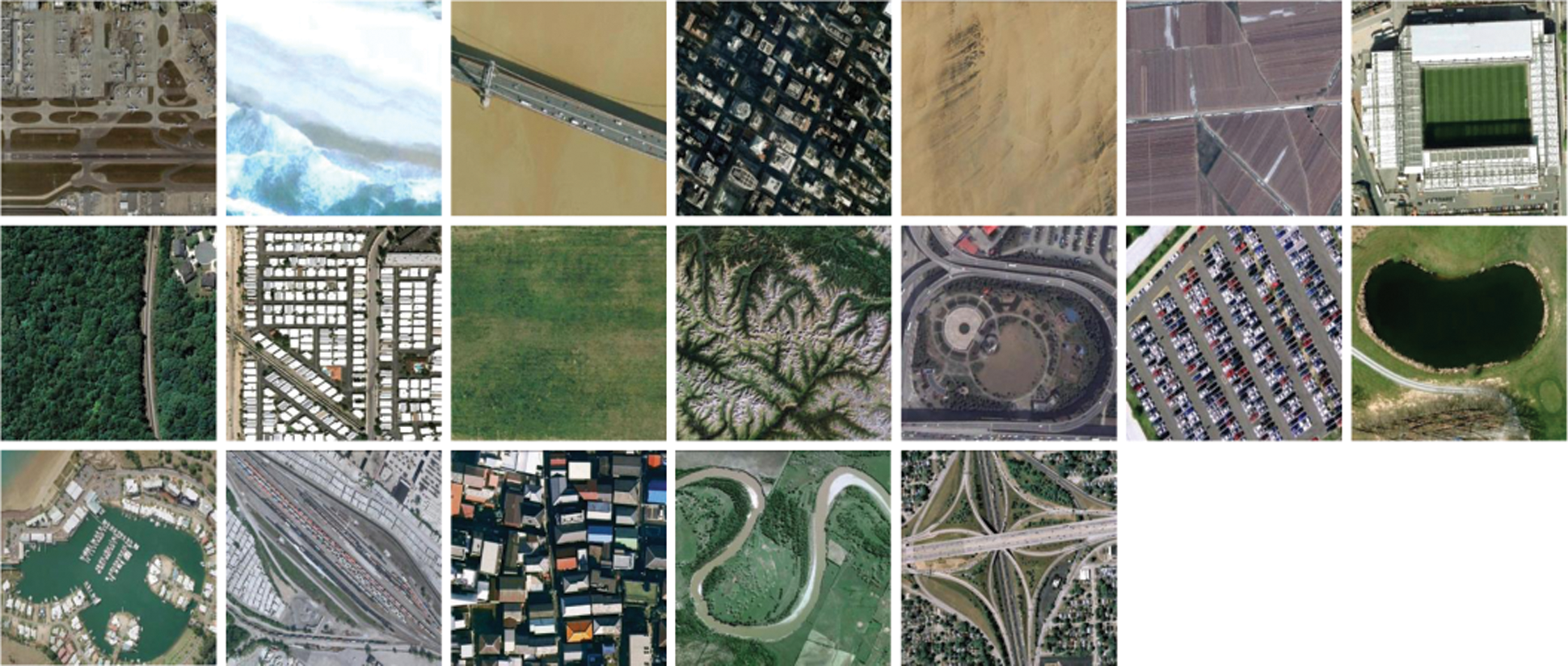
Figure 7: Example image from each class of WHU-RS19 dataset

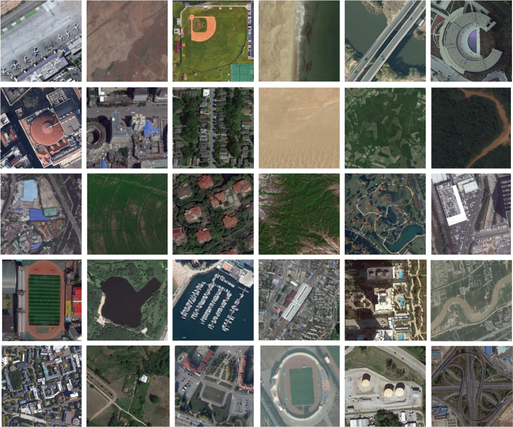
Figure 8: Example image from each class of AID dataset

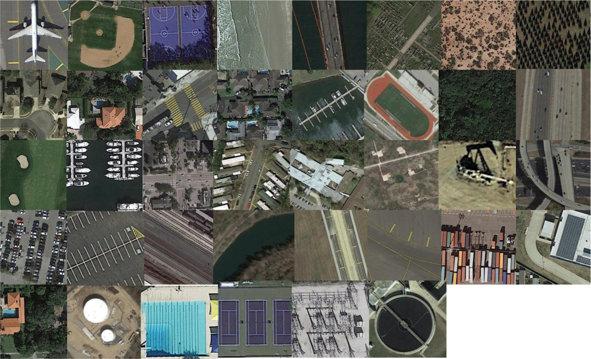
Figure 9: Example image from each class of PatternNet dataset

3.1.2 Performance Evaluation Criteria

The retrieval performance of the proposed descriptor is evaluated using average normalized modified retrieval rank (ANMRR), mean average precision (MAP) and precision-recall (P-R) graph, the details of which are given below:

1.    Average normalized modified retrieval rank (ANMRR)

It is often employed to assess the retrieval performance of MPEG-7 standard and is quite popular in the field of remote sensing image retrieval. The value of ANMRR ranges between 0 and 1. Smaller the value, higher the retrieval efficacy [3,46]. For any query image (q), Gr(q) denotes the size of ground truth images and let the ground truth image at kth position is retrieved at the location Rank(k). Subsequently, the image ranks that are treated as acceptable from retrieval point of view are expressed as K(q) which is two times that of Gr(q) and the images belonging to higher ranks are given a penalty as:

Rank(m)={ Rank(m)if Rank(m)<K(q)1.25K(q)if Rank(m)>K(q) (19)

Therefore the average rank (Ar) for q is given as:

Ar(q)=1Gr(q)∑m=1Gr(q)Rank(m) (20)

To control the effect of variable no. of ground truths of query image, the normalization is done and averaged for all query images NQ to compute ANMRR:

ANMRR=1NQ∑q=1NQAr(q)−0.5[1+Gr(q)]1.25K(q)−0.5[1+Gr(q)] (21)

2.    Mean Average Precision (MAP)

The MAP is one way to congregate Precision-Recall curve into a single value that assess the rank place of all ground truth. Let Prave(q) is the average precision for each query image q which is simply the average of precision values of each relevant item:

Prave(q)=∑k=1n(Pr(k)∗rel(k))No. of relevant items (22)

where rel(k) denotes a function which outputs 1 if the item at kth rank is valid or relevant else outputs 0. The Pr(k) denotes the precision at k. The Prave values over all query items lastly provides the MAP:

MAP=∑q=1NQPrave(q)NQ (23)

The range of MAP value lies between 0 and 100. Higher value of MAP signifies better retrieval performance of the descriptor [3,46].

3.    Precision-Recall (P-R) curve

Precision and recall, both are popularly used for image retrieval performance assessment. The ratio of number of relevant images retrieved to the number of images retrieved gives the precision value whereas recall is the ratio of number of relevant images retrieved to the number of relevant images in a database. The descriptor that shows largest area under the curve indicates high precision and high recall which exhibits better results relevancy and improved correct relevant image retrieval [46].

3.2 Results and Analysis

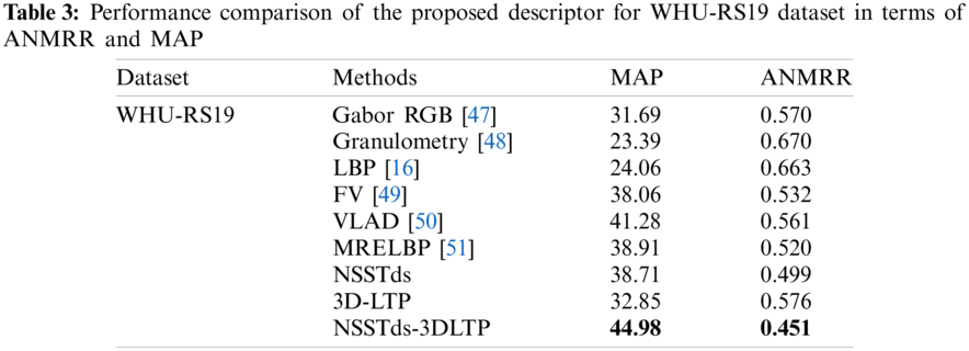
Here for the experiments, the remote sensing images are decomposed using NSST with 3,3,4,4 directions to extract the NSST-domain statistical features. It yields one approximation subband along with 48 detail subbands. For each database, the performance of proposed descriptor is compared with Gabor RGB [47], Granulometry [48], LBP [16], FV [49], VLAD [50] and MRELBP [51] in terms of MAP and ANMRR (Tables 3 and 4).

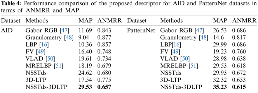
From Tables 3 and 4, it is observed that the global NSSTds features performs better than the local 3D-LTP features both in terms of ANMRR and MAP for WHU-RS19 and AID databases, and both NSSTds and 3D-LTP performs quite close for Patternnet. The good performance of proposed NSSTds features is due to its suitability of capturing texture features for retrieval of remote sensing images and can effectively describe features mainly over multiple scales and multiple orientations. For each database, the proposed fusion NSSTds-3DLTP outperforms all the existing methods including MRELBP which is also known for its ability to capture both global and local features (Tables 3 and 4). The proposed method shows good improvement over other methods both in terms of MAP and ANMRR which verifies the efficacy of combining proposed NSST domain statistical feature and 3D-LTP. In terms of MAP,ANMRR, the NSSTds-3DLTP improves upon Gabor RGB, Granulometry, LBP, FV, VLAD and MRELBP descriptors by 41.93%,20.87%, 92.30%,32.68%, 86.14%,31.97%, 18.18%,15.22%, 8.96%,19.60% and 15.60%,13.26% respectively for WHU-RS19 dataset. For AID, in terms of {MAP,ANMRR}, the NSSTds-3DLTP improves upon Gabor RGB, Granulometry, LBP, FV, VLAD and MRELBP descriptors by {152.60%,22.06%}, {226.65%,25.08%}, {185.03%,23.33%}, {80.06%,12.16%}, {50.58%,10.49%} and {62.34%,3.24%} respectively and for PatternNet dataset the NSSTds-3DLTP respectively improves upon Gabor RGB, Granulometry, LBP, FV, VLAD and MRELBP descriptors by {32.79%, 10.34%}, {141.30%, 24.72%}, {17.47%,10.34%}, {83.20%,19.07%}, {21.56%,3.60%}, and {19.30%,0.48%} in terms of {MAP,ANMRR}. Unlike most of the other methods, which are either local or global, the subfeature 3D-LTP not only encodes the color cue but the local texture information is extracted too. Further, the subfeature NSSTds is capable of capturing the image information at multiple scales and orientations. The complementary characteristics of NSSTds and 3D-LTP are combined in NSSTds-3DLTP to produce a highly discriminative representation.

In Tables 5–7, the average precision of all descriptors including proposed descriptors (NSSTds, 3D-LTP, NSSTds-3DLTP) for individual classes and for each database is shown. The average precision value is calculated for 20 top retrieved images found in 20 trials for 20 images selected randomly from each image class. Tables 5–7 show that the NSSTds-3DLTP features performs best in most of the individual classes compared to other techniques including global NSSTds and local 3D-LTP. From Tables 5–7, it can be clearly seen that the global NSSTds features alone when compared to local 3D-LTP show good performance on the specific classes like Forest, river, residential, bareland, school, mountain, parking etc. which are more texture based and have image-scale attributes (Fig. 10). However, the local 3D-LTP alone when compared to global NSSTds show good performance on the classes like intersection, railway, baseball field, freeway, storage tank, golf course,church, commercial, pond, medium residential, bridge etc. that contains unique arrangement of structures in the absence of which the images cannot be retrieved correctly (Fig. 10). These results confirms that the local and global features contain mutually supportive details and their combination is expected to improve the discriminativeness of features. The retrieval of challenging images such as tennis court, dense residential, sparse residential, stadium, playground etc. are significantly improved using fused NSSTds-3DLTP descriptor. In Fig. 12, a few image query examples from different classes and its corresponding retrieved results using proposed NSSTds-3DLTP descriptor (for all the three databases) are shown. From Fig. 12a, it is observed that the images from the classes beach, bridge, desert, farmland, industrial and river from WHU-RS19 dataset when given as input query images exhibit correct retrieval results except for viaduct class where it provides one incorrect retrieved result, i.e., an image from Railway class is wrongly retrieved here. Likewise, from Fig. 12b, it is observed that the images from the classes airport, bareland, church, dense residential, desert, medium residential and school from AID dataset when given as input query images exhibit correct retrieval results except for Beach class where it provides one incorrect retrieved result i.e., an image from bridge class is wrongly retrieved here. And, from Fig. 12c it is observed that the images from the classes baseball field, beach, cemetry, chaparral, closed road, coastal mansion, waste water treatment plant from PatternNet dataset when given as input query images exhibit correct retrieval results except for Airplane class where it provides one incorrect retrieved result i.e., an image from waste water treatment plant class is wrongly retrieved here. From Tables 3 and 4, Figs. 11 and 12, we can conclude that the NSSTds-3DLTP is able to achieve encouraging results for most of the images over other techniques, however it shows a few cases of incorrect retrieval too in relatively simple class such as ‘beach’.

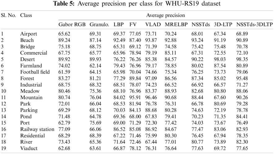
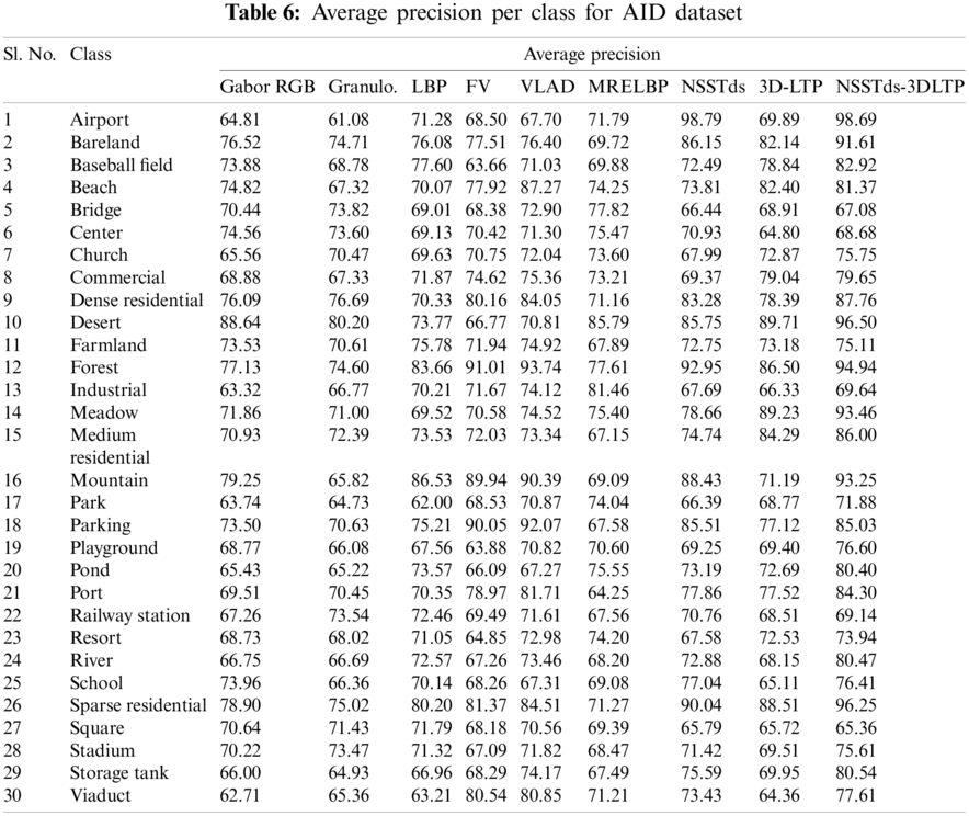
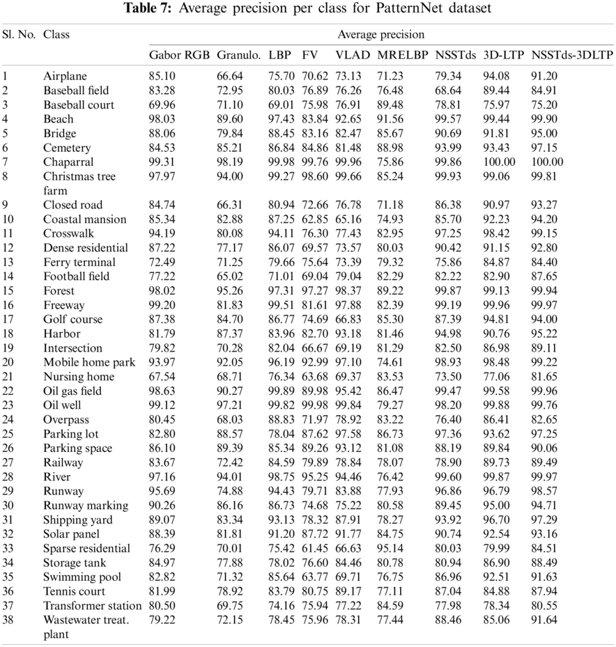
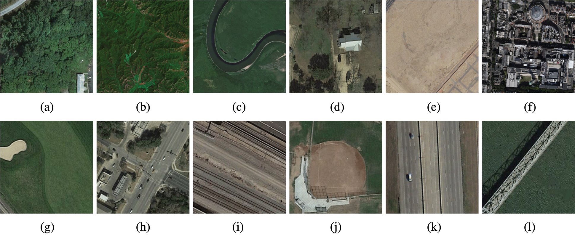
Figure 10: Image classes on which improved results are achieved using global NSSTds alone (1st row) and local 3D-LTP alone (2nd Row) when compared to each other. (a) ‘Forest’ (b) ‘Mountain’ (c) ‘River’ (d) ‘Residential’ (e) ‘Bareland’ (f) ‘School’ (g) ‘Golf Course’ (h) ‘Intersection’ (i) ‘Railway’ (j) ‘Baseball field’ (k) ‘Freeway’ (l) ‘Bridge’

In order to further show the superiority of proposed fused features over other techniques including NSSTds and 3D-LTP, the P-R curves for all the techniques are shown in Figs. 11a–11c for WHU-RS19, AID and PatternNet databases respectively. Precision is defined as the ratio of number of relevant images retrieved to the total number of retrieved images, however recall is defined as the ratio of number of relevant images retrieved to the total number of relevant images present in the database. Precision indicates the accuracy of retrieval and recall indicates about the efficacy of the retrieval performance. The precision-recall graph describes about the inherent trade-off between these two parameters and is an important performance indicator in retrieval systems. The descriptor who has the largest area enclosed by its precision-recall curve (high precision and high recall) is considered as the the superior one.

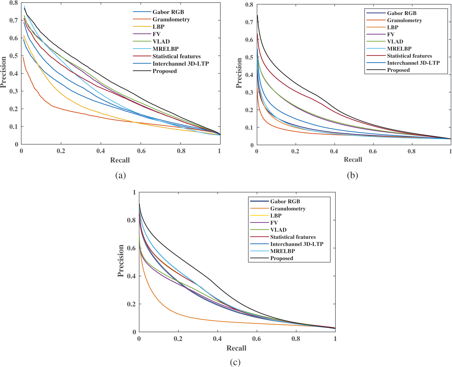
Figure 11: The precision-recall curve for (a) WHU-RS19, (b) AID and (c) PatternNet dataset

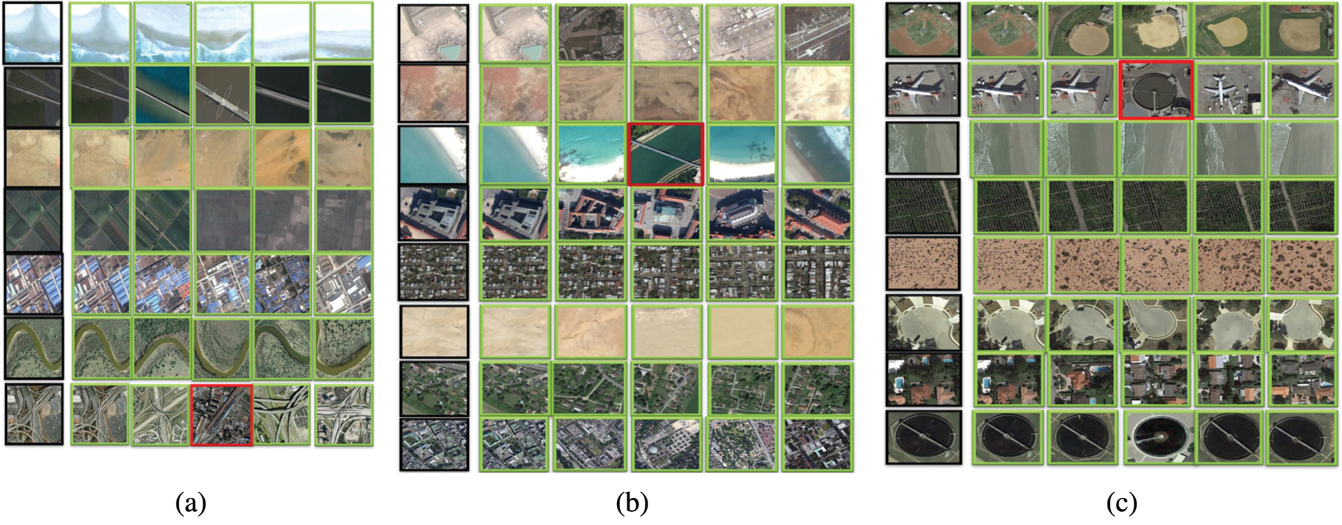
Figure 12: Few cases of input query examples taken from different classes and the corresponding retrieval results using NSSTds-3DLTP (Input query image, correct retrieved results and wrong retrieved results are enclosed in Black, Green and Red coloured boxes respectively for more clarity). (a) WHU-RS19, (b) AID, (c) PatternNet

In Fig. 11a, i.e., for WHU-RS19 dataset, the P-R curve obtained using NSSTds-3DLTP encloses the largest area and exhibits the best results followed by VLAD, FV, NSSTds, MRELBP, 3D-LTP, Gabor RGB, LBP and Granulometery descriptors. For AID dataset, the NSSTds-3DLTP exhibits the superior results followed by NSSTds, VLAD, FV, 3D-LTP, MRELBP, Gabor RGB, LBP and Granulometry (Fig. 11b). Similarly, for PatternNet too, the NSSTds-3DLTP shows the best results followed by MRELBP, 3D-LTP, LBP, NSSTds, VLAD, FV, Gabor RGB and Granulometry (Fig. 11c). The P-R curve results are observed to be consistent with Tables 2 and 3 results.

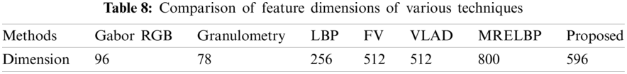
From Table 8, it can be seen that the feature dimensions of NSSTds-3DLTP is less than MRELBP and higher than other techniques. The Gabor RGB, granulometery, LBP, FV and VLAD techniques have comparatively less feature dimensions than NSSTds-3DLTP, but their performance is also well less than NSSTds-3DLTP. The NSSTds-3DLTP outperforms state of the art MRELBP with relatively less feature dimensions.

4  Conclusions

This paper combines global feature based on NSSTds and local feature based on 3D-LTP to generate a combined representation, i.e., NSSTds-3DLTP for retrieval of high-resolution remote sensing image. The complementary characteristics of local and global texture features along with colour information are utilized in NSSTds-3DLTP to produce a highly discriminative representation. Through KS test and log histogram plots we have shown that the 2-state LM distribution is the most appropriate distribution that approximates the statistics of high-frequency detail subband coefficients. Five statistical parameters are extracted from each NSST subband to form the feature vector of NSSTds. The 3D-LTP exploits both local texture details and colour information whereas the NSSTds exploits only global texture information. The image retrieval experiments using WHU-RS19, AID and PatternNet datasets validate the superior performance of NSSTds-3DLTP over many existing techniques with an encouraging margin. The NSSTds-3DLTP achieves the performance without any requirement for a pre-training and without parameter tuning and with less dimensions which is important from real-time implementation point of view.

In the future work, more effective local/global combination will be investigated and the shape based features will be exploited too.

Acknowledgement: The research fellowship support through Visvesvaraya PhD Scheme for Electronics and IT by Digital India Corporation, Ministry of Electronics and Information Technology (MeitY), Government of India is highly acknowledged by the authors.

Funding Statement: The authors received no specific funding for this study.

Conflicts of Interest: The authors declare that they have no conflicts of interest to report regarding the present study.

References

 1.  Ferecatu, M., Boujemaa, N. (2007). Interactive remote-sensing image retrieval using active relevance feedback. IEEE Transactions on Geoscience and Remote Sensing, 45(4), 818–826. DOI 10.1109/TGRS.2007.892007. [Google Scholar] [CrossRef]

 2.  Imbriaco, R., Sebastian, C., Bondarev, E., de With, P. H. N. (2019). Aggregated deep local features for remote sensing image retrieval. Remote Sensing, 11(5), 1–23. DOI 10.3390/rs11050493. [Google Scholar] [CrossRef]

 3.  Baruah, H. G., Nath, V. K., Hazarika, D. (2019). Remote sensing image retrieval via symmetric normal inverse Gaussian modeling of nonsubsampled shearlet transform coefficients. International Conference on Pattern Recognition and Machine Intelligence, pp. 359–368. Tezpur, India. [Google Scholar]

 4.  Xiong, W., Lv, Y., Cui, Y., Zhang, X., Gu, X. (2019). A discriminative feature learning approach for remote sensing image retrieval. MDPI Remote Sensing, 11(3), 1–19. DOI 10.3390/rs11030281. [Google Scholar] [CrossRef]

 5.  Lowe, D. G. (2004). Distinctive image features from scale-invariant keypoints. International Journal of Computer Vision, 60, 91–110. DOI 10.1023/B:VISI.0000029664.99615.94. [Google Scholar] [CrossRef]

 6.  Swain, M. J., Ballard, D. H. (1991). Color indexing. International Journal of Computer Vision, 7, 11–32. DOI 10.1007/BF00130487. [Google Scholar] [CrossRef]

 7.  Oliva, A., Torralba, A. (2006). Building the gist of a scene: The role of global image features in recognition. Progress in Brain Research, 155, 23–36. DOI 10.1016/S0079-6123(06)55002-2. [Google Scholar] [CrossRef]

 8.  Navneet, D., Bill, T. (2005). Histograms of oriented gradients for human detection. IEEE Computer Vision and Pattern Recognition, pp. 886–893. San Diego, CA, USA. [Google Scholar]

 9.  Ojala, T., Matti, P., Topi, M. (2002). Multiresolution gray-scale and rotation invariant texture classification with local binary patterns. IEEE Transactions on Pattern Analysis & Machine Intelligence, 24(7), 971–987. DOI 10.1109/TPAMI.2002.1017623. [Google Scholar] [CrossRef]

10. Ma, A., Sethi, I. K. (2005). Local shape association based retrieval of infrared satellite images. 7th IEEE International Symposium on Multimedia, pp. 551–557. Irvine, CA, USA. [Google Scholar]

11. Yang, F. P., Hao, M. L. (2017). Effective image retrieval using texture elements and color fuzzy correlogram. Information, 8(1), 1–11. DOI 10.3390/info8010027. [Google Scholar] [CrossRef]

12. Choy, S. K., Tong, C. S. (2010). Statistical wavelet subband characterization based on generalized gamma density and its application in texture retrieval. IEEE Transactions on Image Processing, 19(2), 281–289. DOI 10.1109/TIP.2009.2033400. [Google Scholar] [CrossRef]

13. Allili, M. S. (2012). Wavelet modeling using finite mixtures of generalized Gaussian distributions: Application to texture discrimination and retrieval. IEEE Transactions on Image Processing, 21(4), 1452–1464. DOI 10.1109/TIP.2011.2170701. [Google Scholar] [CrossRef]

14. Liu, Z., Zhu, L. (2018). A novel retrieval method for remote sensing image based on statistical model. Multimedia Tools and Applications, 77, 24643–24662. DOI 10.1007/s11042-018-5649-6. [Google Scholar] [CrossRef]

15. Haindl, M., Vacha, P. (2006). Illumination invariant texture retrieval. 18th International Conference on Pattern Recognition, pp. 276–279. Hong Kong, China. [Google Scholar]

16. Ojala, T., Pietikainen, M., Maenpaa, T. (2002). Multiresolution gray-scale and rotation invariant texture classification with local binary patterns. IEEE Transactions on Pattern Analysis and Machine Intelligence, 24(7), 971–987. DOI 10.1109/TPAMI.2002.1017623. [Google Scholar] [CrossRef]

17. Tan, X., Triggs, B. (2010). Enhanced local texture feature sets for face recognition under difficult lighting conditions. IEEE Transactions on Image Processing, 19(6), 1635–1650. DOI 10.1109/TIP.2010.2042645. [Google Scholar] [CrossRef]

18. Chen, C., Zhang, B., Su, H., Li, W., Wang, L. (2016). Land-use scene classification using multi-scale completed local binary patterns. Signal, Image and Video Processing, 10, 745–752. DOI 10.1007/s11760-015-0804-2. [Google Scholar] [CrossRef]

19. Huang, L., Chen, C., Li, W., Du, Q. (2016). Remote sensing image scene classification using multi-scale completed local binary patterns and fisher vectors. MDPI Remote Sensing, 8(6), 1–17. DOI 10.3390/rs8060483. [Google Scholar] [CrossRef]

20. Yang, J., Liu, J., Dai, Q. (2015). An improved bag-of-words framework for remote sensing image retrieval in large-scale image databases. International Journal of Digital Earth, 8(4), 273–292. DOI 10.1080/17538947.2014.882420. [Google Scholar] [CrossRef]

21. Sukhia, K. N., Riaz, M. M., Ghafoor, A., Ali, S. S. (2020). Content-based remote sensing image retrieval using multi-scale local ternary pattern. Digital Signal Processing, 104, 102765. DOI 10.1016/j.dsp.2020.102765. [Google Scholar] [CrossRef]

22. Wang, Y., Zhang, L., Tong, X., Zhang, L., Zhang, Z. et al. (2016). A three-layered graph-based learning approach for remote sensing image retrieval. IEEE Transactions on Geoscience and Remote Sensing, 54(10), 6020–6034. DOI 10.1109/TGRS.2016.2579648. [Google Scholar] [CrossRef]

23. Bosilj, P., Aptoula, E., Lefèvre, S., Kijak, E. (2016). Retrieval of remote sensing images with pattern spectra descriptors. ISPRS International Journal of Geo-Information, 5(12), 1–16. DOI 10.3390/ijgi5120228. [Google Scholar] [CrossRef]

24. Bian, X., Chen, C., Tian, L., Du, Q. (2017). Fusing local and global features forhigh-resolution scene classification. IEEE Journal of Selected Topics in Applied Earth Observations and Remote Sensing, 10(6), 2889–2901. DOI 10.1109/JSTARS.4609443. [Google Scholar] [CrossRef]

25. Risojevic, V., Babic, Z. (2013). Fusion of global and local descriptors for remote sensing image classification. IEEE Geoscience and Remote Sensing Letters, 10(4), 836–840. DOI 10.1109/LGRS.2012.2225596. [Google Scholar] [CrossRef]

26. Liu, L., Lao, S., Fieguth, P. W., Guo, Y., Wang, X. et al. (2016). Median robust extended local binary patternfor texture classification. IEEE Transactions on Image Processing, 25(3), 1368–1381. DOI 10.1109/TIP.2016.2522378. [Google Scholar] [CrossRef]

27. Yang, P., Yang, G. (2018). Statistical model and local binary pattern based texture feature extraction in dual-tree complex wavelet transform domain. Multidimensional Systems Signal Processing, 29, 851–865. DOI 10.1007/s11045-017-0474-z. [Google Scholar] [CrossRef]

28. Kabbai, L., Abdellaoui, M., Douik, A. (2019). Image classification by combining local and global features. The Visual Computer, 35, 679–693. DOI 10.1007/s00371-018-1503-0. [Google Scholar] [CrossRef]

29. Yan, X., Jiangtao, P., Qian, D. (2020). Multiple feature regularized kernel for hyperspectral imagery classification. APSIPA Transactions on Signal and Information Processing, 9, 1–8. DOI 10.1017/ATSIP.2020.8. [Google Scholar] [CrossRef]

30. Zeng, D., Chen, S., Chen, B., Li, S. (2018). Improving remote sensing scene classification by integrating global-context and local-object features. MDPI Remote Sensing, 10(5), 1–19. DOI 10.3390/rs10050734. [Google Scholar] [CrossRef]

31. Lv, Y., Zhang, X., Xiong, W., Cui, Y., Cai, M. (2019). An end-to-end local-global-fusion feature extraction network for remote sensing imagescene classification. MDPI Remote Sensing, 11, 3006(24), 1–20. DOI 10.3390/rs11243006. [Google Scholar] [CrossRef]

32. Wang, X., Tao, J., Shen, Y., Bai, S., Song, C. (2019). A nsst pansharpening method based on directional neighborhood correlation and tree structure matching. Multimedia Tools and Applications, 78(18), 26787–26806. DOI 10.1007/s11042-019-07841-5. [Google Scholar] [CrossRef]

33. Candes, E., Demanet, L., Donoho, D., Ying, L. (2006). Fast discrete curvelet transforms. Multiscale Modeling & Simulation, 5(3), 861–899. DOI 10.1137/05064182X. [Google Scholar] [CrossRef]

34. Do, M. N., Vetterli, M. (2005). The contourlet transform: An efficient directional multiresolution image representation. IEEE Transactions on Image Processing, 14(12), 2091–2106. DOI 10.1109/TIP.2005.859376. [Google Scholar] [CrossRef]

35. Easley, G., Labate, D., Lim, W. Q. (2008). Sparse directional image representations using the discrete shearlet transform. Applied and Computational Harmonic Analysis, 25(1), 25–46. DOI 10.1016/j.acha.2007.09.003. [Google Scholar] [CrossRef]

36. Hou, B., Zhang, X., Bu, X., Feng, H. (2012). Sar image despeckling based on nonsubsampled shearlet transform. IEEE Journal of Selected Topics in Applied Earth Observations and Remote Sensing, 5(3), 809–823. DOI 10.1109/JSTARS.4609443. [Google Scholar] [CrossRef]

37. Farhangi, N., Ghofrani, S. (2018). Using bayesshrink, bishrink, weighted bayesshrink, and weighted bishrink in nsst and swt for despeckling sar images. EURASIP Journal on Image and Video Processing, 2018(4), 1–18. DOI 10.1186/s13640-018-0244-3. [Google Scholar] [CrossRef]

38. Hazarika, D. (2017). Despeckling of synthetic aperture radar (SAR) images in the lapped transform domain (Ph.D. Thesis). Tezpur University, India. [Google Scholar]

39. Rabbani, H., Vafadust, M., Abolmaesumi, P., Gazor, S. (2008). Speckle noise reduction of medical ultrasound images in complex wavelet domain using mixture priors. IEEE Transactions on Biomedical Engineering, 55(9), 2152–2160. DOI 10.1109/TBME.10. [Google Scholar] [CrossRef]

40. Banerji, S., Sinha, A., Liu, C. (2013). New image descriptors based on color, texture, shape, and wavelets for object and scene image classification. Neurocomputing, 117, 173–185. DOI 10.1016/j.neucom.2013.02.014. [Google Scholar] [CrossRef]

41. WHU-RS19 (2018). http://dsp.whu.edu.cn/cn/staff/yw/hrsscene.html. [Google Scholar]

42. Xia, G. S., Hu, J., Hu, F., Shi, B., Bai, X. et al. (2017). Aid: A benchmark data set for performance evaluation of aerial scene classification. IEEE Transactions on Geoscience and Remote Sensing, 55(7), 3965–3981. DOI 10.1109/TGRS.2017.2685945. [Google Scholar] [CrossRef]

43. AID (2018). http://www.lmars.whu.edu.cn/xia/aid-project.html. [Google Scholar]

44. Zhou, W., Newsam, S., Li, C., Shao, Z. (2018). Patternnet: A benchmark dataset for performance evaluation of remote sensing image retrieval. ISPRS Journal of Photogrammetry and Remote Sensing, 145, 197–209. DOI 10.1016/j.isprsjprs.2018.01.004. [Google Scholar] [CrossRef]

45. PatternNet (2018). https://sites.google.com/view/zhouwx/dataset. [Google Scholar]

46. Napoletano, P. (2018). Visual descriptors for content-based retrieval of remote sensing images. International Journal of Remote Sensing, 39(5), 1343–1376. DOI 10.1080/01431161.2017.1399472. [Google Scholar] [CrossRef]

47. Bianconi, F., Fernández, A. (2007). Evaluation of the effects of gabor filter parameters on texture classification. Pattern Recognition, 40(12), 3325–3335. DOI 10.1016/j.patcog.2007.04.023. [Google Scholar] [CrossRef]

48. Hanbury, A., Kandaswamy, U., Adjeroh, D. A. (2005). Illumination-invariant morphological texture classification. In: Mathematical morphology: 40 years on, pp. 377–386. DOI 10.1007/1-4020-3443-1. [Google Scholar] [CrossRef]

49. Florent, P., Jorge, S., Thomas, M. (2010). Improving the fisher kernel for large-scale image classification. European Conference on Computer Vision, pp. 143–156. Heraklion, Crete, Greece. [Google Scholar]

50. Hervé, J., Matthijs, D., Cordelia, S., Patrick, P. (2010). Aggregating local descriptors into a compact image representation. IEEE Computer Society Conference on Computer Vision and Pattern Recognition, pp. 3304–3311. San Francisco, CA, USA. [Google Scholar]

51. Liu, L., Lao, S., Fieguth, P. W., Guo, Y., Wang, X. et al. (2016). Median robust extended local binary pattern for texture classification. IEEE Transactions on Image Processing, 25(3), 1368–1381. DOI 10.1109/TIP.2016.2522378. [Google Scholar] [CrossRef]

This work is licensed under a Creative Commons Attribution 4.0 International License, which permits unrestricted use, distribution, and reproduction in any medium, provided the original work is properly cited.