Computer Modeling in Engineering & Sciences

DOI: 10.32604/cmes.2022.019069

ARTICLE

N-SVRG: Stochastic Variance Reduction Gradient with Noise Reduction Ability for Small Batch Samples

Haijie Pan and Lirong Zheng*

School of Information Science and Engineering, Fudan University, Shanghai, 200433, China
*Corresponding Author: Lirong Zheng. Email: lrzheng@fudan.edu.cn
Received: 01 September 2021; Accepted: 11 October 2021

1  Introduction

The variance problem introduced by the stochastic nature of the SGD algorithm becomes the main problem of optimization algorithms nowadays. The introduction of variance makes SGD reach only sublinear convergence speed with a fixed step size [1], while the stochastic algorithm accuracy is positively related to the sampling variance, and when the variance tends to 0, the deviation of the algorithm will also be 0. In this case, the SGD can still be fast even with a large step size convergence. Therefore, how to reduce the variance of the stochastic gradient in the stochastic algorithm has become an important issue studied by scholars [2].

For SGD variance problem, there are three mainstream methods to reduce the variance of sampling at present that include importance sampling, hierarchical sampling method and control variable method. The objective function in machine learning is usually solved using the Batch Gradient Descent (BGD) or SGD [3]. BGD algorithm computes the gradients of all samples for each iteration to perform the weight update, and the latter randomly selects one training sample at a time to update the parameters by computing the sample gradients. Then came the improved Mini-Batch SGD (MBGD) algorithm, where MBGD computes the gradient and performs weight update by randomly selecting m data samples in the original data for each iteration. SGD has the advantage that each step relies only on a simple random sample gradient, so the computational consumption is only a fraction of that of the standard GD [4]. However, it has the disadvantage that a constant step size leads to slow convergence in the case of variance introduced by randomness.

In recent years, many scholars have carried out research based on SGD algorithm, for example, momentum algorithm [5], which is based on the idea of gradient momentum accumulation and uses exponential weighted average to reduce the swing amplitude of the gradient. Two concepts of velocity and friction are introduced into momentum algorithm. The function of the gradient is to change velocity, and friction is to gradually reduce the velocity. In the whole training process, the increase and attenuation of momentum are simulated to achieve the purpose of convergence. AdaGrad (Adaptive Gradient) is proposed to learn by gradually decreasing the step size [6]. By accumulating gradients, the learning rate of each weight is related to the value of their previous gradient. However, the consequence of accumulating gradients is that as the training increases, the step size decreases and eventually the training stalls. To address the training stagnation problem that occurs with AdaGrad, Hinton, G. proposed RMSProp (Root Mean Square Prop) to calculate the cumulative gradient using a moving average method that only accumulates the gradient of one window, making the change in step size adapt to the current gradient thus achieving better optimization [7,8]. And for SGD stochasticity introduces the variance problem, where SVRG is used to correct the gradient used for each model update using the global average gradient information [9]. Theoretical analysis and experiments demonstrated that SVRG produced linear convergence with reducing variance. Subsequently, Zhao et al. [10] proposed the SASG (Stochastic Average Gradient Average) algorithm, which has the same thematic idea as SVRG, with the difference that a piece of memory is used to store the original gradients of all samples, and the global average gradient is updated by constantly updating the original gradients during training, which requires a large amount of memory consumption throughout the training [11]. The SCSG (Stochastically Controlled Sto-chastic Gradient) algorithm was proposed, SCSG is to calculate the average gradient by randomly selecting a part of the sample gradient as the global gradient, but when performing the weight update, randomly selecting the number of updates will make the calculation more variable and tedious, and the computation is large [12]. Subsequently, a series of algorithms [13] such as the novel Mini-Batch SCSG [14,15], b-NICE, SAGA [16,17] were generated based on the idea of variance reduction.

However, there is another structural risk minimization problem in machine learning, which is composed of “loss function + regularization term”, and different forms of regularization terms lead to different complex problems, such as Overlapping group lasso, Graph-guided fused lasso etc. [18], which are very complex for SGD-based theoretical approaches, while the ADMM algorithm is applied to a wider range of models and its excellent performance proves itself to be an effective optimization tool. Several variance reduction algorithms have been proposed in combination with ADMM, including SAG-ADMM [19], SDCA-ADMM [20], and SVRG-ADMM [21]. All three algorithms are improved algorithms generated based on the update strategy of ADMM. Then [22] proposed the APA-SVRG, which is trained on the basis of SVRG using proximity averaging, and the experimental results show that the APA-SVRG algorithm is comparable to SVRG-ADMM. The neighborhood stochastic L-BFGS [23] methods, on the other hand, an improved algorithm based on Newton’s method, which is trained mainly on loss functions that are smooth functions. Meanwhile, the specular stochastic sub-gradient descent [24] method is used to train on the loss function that is a non-smooth function. However, these schemes compute the gradient unbiased estimation using the average gradient of a small batch of samples, which cannot reduce the total complexity linearly, and the computational cost and memory consumption increase, and the computation and update of the gradient of a small batch of samples increase the computational consumption of the whole algorithm [25].

In order to address the above challenges, we propose a noise reduction method of stochastic gradient method, and then use the idea of small sample average gradient instead of global average gradient to design the algorithm N-SVRG that selects small samples for training while updating the average gradient to achieve variance reduction, and introduce the algorithm flow and convergence analysis of N-SVRG algorithm in detail, and compare it with the mainstream Mini-Batch SGD The N-SVRG algorithm is compared with the mainstream Mini-Batch SGD, AdaGrad, RMSProp, SVRG and SCSG algorithms, and it is proved that the N-SVRG algorithm outperforms SVRG, SASG and other algorithms, and is equal to SCSG. Finally, by exploring the relationship between the small values of different parameters n. B and k and the effectiveness of the algorithm, we prove that the N-SVRG algorithm has some stability and can achieve sufficient accuracy even in the case of low back size. Experimentally comparing the advantages and disadvantages of various methods and exploring the stability of the N-SVRG algorithm through parameter settings.

The contributions of this paper are as follows:

* We propose N-SVRG that uses small batches samples instead of all samples for the average gradient calculation, while performing an incremental update of the average gradient. By suitably reducing the batch size B, the memory storage as well as the number of iterations can be reduced.

* The convergence analysis of the proposed algorithm shows that the algorithm can stably converge to a certain lower limit, and find the saddle point with smooth gradient descent in the whole training process of neural network. It also enables the algorithm in this paper to reduce the computational cost and memory burden.

* The experiments are compared with the state-of-the-art demonstrate that N-SVRG outperforms baseline. Exploring the relationship between the small values of different parameters n. B and k and the effectiveness of the algorithm, we prove that our N-SVRG algorithm has some stability and can achieve sufficient accuracy even in the case of low batch size.

2  Background

For the supervised learning problem in machine learning [2,26]: assume that there is a functional model l in the space L for each model input x, i.e., there is a prediction l(x). That is, given n training data (x1,y1),(x2,y2),⋯,(xn,yn) where xi∈Rd denotes the input sample data and yi∈R denotes the corresponding training labels. Our goal is to find the prediction function that minimizes the loss due to inaccurate predictions. However, since the predictions l(x) and yi will differ each time the model predicts, one uses the loss function to assess the difference between the two. Since each sample corresponds to a loss function, the empirical risk is the average of these n sample loss functions.

Experience risk:

Pn(w)=1n∑i=1nfi(l(w;xi),yi) (1)

Expected risk:

P(w)=E[fi(l(w;xi),yi)] (2)

where w represents the parameters in the function model, and fi(l(w;xi,yi)) represents the loss function corresponding to sample (xi,yi). Formulas (1) and (2) clearly show how the expected risk and empirical risk depend on the error function, sample space, sample set, etc.

Empirical risk minimization is solving for w such that the empirical risk is minimized:

w∗∈arg minw(P(w):=1n∑i=1nfi(w;xi,yi)) (3)

However, during the training process, the model may have a strong performance capability because it has a large number of parameters itself, but the data provided for training are insufficient. Insufficient data for training, then the model may overfit during a large number of repeated training sessions, i.e., “the learned model is so well suited to a specific set of data that it does not reliably fit other data or future observations”. In order to reduce the impact of overfitting [4,27] to some extent, a regularization term is added to the empirical risk to limit the complexity of the model, which constitutes a structural risk minimization [28] in the form of “loss function + regularization term” problem:

w∗∈arg minw(P(w):=1n∑i=1nfi(w;xi,yi)+λr(w)) (4)

where λ > 0 is a hyperparameter that balances the weight of the regularization term by its own numerical size, and the larger λ is set, the heavier the penalty on the weight. r(w) picks different forms depending on the effect, which include L1 parametrization, L2 parametrization [29], and L~∞ parametrization. The most common form is the L2 parametrization, i.e., r(w) = ‖ w ‖ 2, which can be calculated using w12+w22+wn22.

The loss function in machine learning is a non-negative real function f(l(x),y), where the common loss functions are log Logi Loss, Squared Loss, 0-1 Loss, and Loss and Cross Entropy Error Loss (CEL) [30]. As shown below:

Logarithmic loss function:

f(l(x),y)=log⁡(1+exp⁡(−yl(x))) (5)

Mean square error loss function:

f(l(x),y)=(y−l(x))2 (6)

0-1 Loss function:

f(l(x),y)={1l(x)≠y0l(x)=y (7)

Cross-entropy error loss function:

f(l(x),y)=−ylog⁡(l(x)) (8)

The use of these loss functions should be chosen according to the specific problem, for example, the cross-entropy error loss function can be used with the Softmax function to form a Softmax-with-Loss layer for training and learning the classification problem [31].

3  Related Concepts

To facilitate the subsequent analysis and study, we give the relevant basic concepts that will be covered in the paper as well as the definitions. There is an iterative sequence xt, with two adjacent iteration points xk+1, xk, satisfying the following conditions:

limk→∞xk+1−x∗xk−x∗=μ (9)

1) If μ = 1, the algorithm achieves sublinear convergence;

2) If 0 < μ < 1, the algorithm achieves linear convergence [32];

3) If μ = 0, the algorithm achieves superlinear convergence.

Let set C⊂Rd, any x1∈C,x2∈C and θ ∈ [0,1] has (1−θ)x1+C,x2∈C, the set C is called a convex set.

Let set C⊂Rd be a convex set and f be a function defined on set C. For any set, x1∈C,x2∈C exists:

f(α1x1+α2x2)≤α1f(x1)+α2f(x2)∑αi=1,αi≥0 (10)

f (x) is a convex function defined on a convex set C.

For a function f(y) with step η > 0, its proximal operator at the point x [33] (Proximal Operator) is defined as:

proxfη(x)=arg miny∈Rd(f(y)+12η‖y−x‖2) (11)

If f=IC is a schematic function on the convex set C

IC(x)={0x∈C+∞x∉C (12)

Then:

proxICη(x)=arg miny∈R(‖y−x‖2) (13)

That is, the proximity operator of the function f(y) at x can be viewed as the Euclidean projection of x on the set C.

Assume (Lipschitz continuous target gradient) that the objective function F: Rd→R is continuously differentiable, the gradient function ∇F:Rd→R of F is Lipschitz continuous and the Lipschitz constant L > 0, i.e.,

‖∇F(w)−∇F(w¯)‖2≤L‖w−w¯‖2,{w,w¯}⊂Rd (14)

Ensures that the gradient of F does not change arbitrarily fast with respect to the parameter vector. This assumption is essential for the convergence analysis of most gradient-based methods; without it, the gradient will not be a good indication of the distance to reduce F.

Assumption 1: If the function fi satisfies L smooth, then for any x,y∈Rd, and fi with gradient ∇fi(x) at point x, there exists L > 0 such that

fi(y)≤fi(x)+⟨∇fi(x),y−x⟩+L2‖y−x‖2 (15)

The constant L is called the Lipschitz constant and is generally used to measure the smoothness of a function. The function satisfies L smoothness in case it itself satisfies the Lipschitz continuity condition. For a fixed fi, L is a fixed value. This condition places a restriction on the variation of the value of the function.

If the function fi is strongly convex, then for any x,y∈Rd, and fi with gradient ∇fi(x) at point x, there exists γ > 0 such that

fi(y)≥fi(x)+⟨∇fi(x),y−x⟩+γ2‖y−x‖2 (16)

4  The Proposed Algorithm

4.1 Controlled Variable Method

This section describes the specific implications of the control variables approach [34]. It is assumed that we need to use Monte Carlo [35] sampling method to estimate the expectation μ of the random variable X, i.e., E[X] = μ. Also assume that we have been able to be able to estimate relatively easily the expectation τ of another random variable Y, i.e., E[Y] = τ. We construct a new random variable:

Z=X+c(Y−τ) (17)

where C∈Rd is the corresponding coefficient, it can be seen from Eq. (17) that Z remains an unbiased estimator of μ [16] and that the variance of Z:

Var(Z)=Var(X)+c2Var(Y)+2cCov(X,Y) (18)

It can be easily obtained by calculation that Var(Z) is minimum at C=−Cov(X,Y)Var(Y), when

Var(Z)=Var(X)−[Cov(X,Y)]2Var(Y)=(1−ρX,Y2)Var(X) (19)

where ρX,Y=Corr(X,Y). It can be seen from (18) and (19). The new random variables Z and X are unbiased estimates of μ as well, but the variance of the random variable Z is smaller than that of X. Therefore, it is better to use the random variable Z as an unbiased estimate of μ than X. From the formula, it can be seen that the variance of Z is sufficiently small as long as the random variable X is guaranteed to show a certain correlation with Y [3], so Y is also called the control variable of X. This is the control variable method.

4.2 SVRG

SVRG is a new variance reduction method formed based on the control variable method, which itself does not construct control variables from similar samples, but from the perspective of optimizing variables. Its iterative approach is:

g˜j−1←∇fij(wj−1)−(∇fij(wt−1)−μ˜)wj←wj−1−ηg˜j−1 (20)

where w∈Rd denotes the model parameters, η denotes the update step, μ˜=∇Rn(wt−1)=1n∑i=1n∇fi(w˜t−1) is the global average gradient which is calculated using the model parameters w˜t−1 obtained at the end of the previous cycle, ∇fi(w˜t−1) denotes the gradient of the function f over the sample ij with respect to parameter w˜t−1, ∇fi(w˜t−1)−μ˜ is the deviation of the control variables from the unbiased estimate, and g˜j−1 is the corrected unbiased estimate, using g˜j−1 to update wj.

SVRG itself is a periodic algorithm, with the increase of iterations, w˜t−1 and wj−1 gradually converge to w∗, that is: w˜t−1→w∗, wj−1→w∗, when t→∞, so ∇fi(wj−1) and ∇fi(w˜t−1) are getting closer and closer, and because ∇fi(wj−1) is the control variable of ∇fi(w˜t−1), according to the theory, when and the closer, the higher the correlation between the two, then the g˜j−1 variance will converge to 0, so that the variance can be reduced to 0 by the control variable method, so the SVRG algorithm achieves linear convergence.

The SVRG algorithm steps are as follows:

Step 1: Given the initialization weight w˜0, the number of SGD steps m, the number of outer loop iterations T and the learning step η, initialize t = 0;

Step 2: Calculate the global average gradient μ˜←∇P(wt−1)=1n∑i=1n∇fi(wt−1) and initialize w0←w˜t−1;

Step 3: j = 0, select a random sample ij∈{1,⋯,n}, calculate g˜j−1=∇fij(wj−1)−(∇fij(wt−1)−μ˜),wj=wj−1−ηg˜j−1,j=j+1, cycle Step 3 until j=m, w˜t←wj, go to the next step;

Step 4: t = t + 1, go to Step 2 until t = T, output: Choice 1: w∗=W˜t+1; Choice 2: w∗=1T∑i=0TW˜t+1. From the pseudo-code, we can see that the main calculations of the algorithm are in Steps 2 and 3, where Step 2 is to calculate the average gradient and Step 3 is used to calculate the corrected unbiased estimate of the gradient from W˜t−1 to W˜t rounds iteratively at a computational cost of n + 2m.

Assuming that all fi are convex functions and satisfy Eqs. (19) and (20) and γ > 0, and assuming that m is large enough, then

α=1γη(1−2Lη)m+2Lη1−2Lη<1 (21)

Expectation of geometric convergence [21] for SVRG:

(P(wt))≤E(P(w∗))+αt[P(w0)−P(w∗)] (22)

Proof: For any i, consider that there is

gi(w)=fi(w)−fi(w∗)−∇fi(w∗)T(w−w∗) (23)

science ∇gi(w∗)=0, so gi(w∗)=minwgi(w),

Because ∇gi(w∗)=0, therefore gi(w∗)=minwgi(w), therefore

0=gi(w∗)≤minη[gi(w)−η‖∇gi(w)‖22]≤minη[gi(w)−η‖∇gi(w)‖22+0.5Lη2‖∇gi(w)‖22]=gi(w)−12L‖∇gi(w)‖22 (24)

So

‖∇fi(w)−∇fi(w∗)‖22≤2L[fi(w)−fi(w∗)−∇fi(w∗)T(w−w∗)] (25)

When i = 1,2, …, n, the cumulative inequality (21) is added. And using ∇P(w∗)=0, we obtain

1n∑i=1n‖∇fi(w)−∇fi(w∗)‖22≤2L[P(w)−P(w∗)] (26)

Give way g˜j−1=∇fij(wj−1)−(∇fij(wt−1)−μ˜) available

Make g˜j−1=∇fij(wj−1)−(∇fij(wt−1)−μ˜) available to

E‖g˜j−1‖22≤2E‖∇fij(wj−1)−∇fij(w∗)‖22+2E‖[∇fij(wt−1)−∇fij(w∗)]−∇P(wt−1)‖22≤2E‖∇fij(wj−1)−∇fij(w∗)‖22+2E‖[∇fij(wt−1)−∇fij(w∗)]−E[∇fij(wt−1)−∇fij(w∗)]‖22≤2E‖∇fij(wj−1)−∇fij(w∗)‖22+2E‖∇fij(wt−1)−∇fij(w∗)‖22≤4L[P(wj−1)−P(w∗)+P(wt−1)−P(w∗)] (27)

The first inequality uses ‖a+b‖22≤2‖a‖22+2‖b‖22μ˜=∇P(wt−1), the second inequality uses

E‖ξ−Eξ‖22=E‖ξ‖22−‖Eξ‖22≤E‖ξ‖22, the third inequality uses (27). Existing

wj=wj−1−ηg˜j−1,E(g˜j−1)=∇P(wj−1), so

E‖wj−V‖22=‖wj−1−w∗‖22−2η(wj−1−w∗)TEg˜j−1+η2E‖g˜j−1‖22≤‖wj−1−w∗‖22−2η(wj−1−w∗)T∇P(wj−1)+4Lη2[P(wj−1)−P(w∗)]+[8+C(j−1)]Lη2[P(wt−1)−P(w∗)]≤‖wj−1−w∗‖22−2η[P(wj−1)−P(w∗)]+4Lη2[P(wj−1)−P(w∗)+P(wt−1)−P(w∗)]=‖wj−1−w∗‖22−2η(1−2 Lη)[P(wj−1)−P(w∗)]+4Lη2[P(wt−1)−P(w∗)] (28)

The first inequality uses the previously obtained inequality E‖g˜j−1‖22, and the second inequality uses the P(w)-convex property. By accumulating the j = 1, … m, stages we obtain

E‖wm−w∗‖22+2ηm(1−2Lη)E[P(wt)−P(w∗)]≤E‖w0−w∗‖22+4Lmη2E[P(wt−1)−P(w∗)]≤2γE[P(wt−1)−P(w∗)]+4Lmη2E[P(wt−1)−P(w∗)=[2γ+2Lmη2]E[P(wt−1)−P(w∗)] (29)

The second inequality uses the strong convexity property, thus obtaining

E[P(wt)−P(w∗)]≤[1γη(1−2Lη)m+2Lη1−2Lη]E[P(wt−1)−P(w∗)] (30)

So get E(P(w˜t))≤E(P(w∗))+αt[P(w0)−P(w∗)], cite as evidence.

5  N-SVRG Algorithm

The SASG algorithm is a memory-consuming algorithm in the SVRG family of algorithms. Although the computational cost of the SVRG algorithm is huge when computing the average of all sample gradients, it can be computed in parallel during the computation because it can use matrix operations itself. the difference between the SASG and SVRG algorithms is that the SASG algorithm requires one memory block to store all sample gradients, which not only increases the computational cost (because matrix parallelism cannot be used), but also increases the memory burden of the computer. In order to reduce the computational cost and memory burden, we designed the back decimation update gradient [2,33].

5.1 Algorithm Introduction

In the SASG algorithm, a piece of memory is used to store the original gradients of all samples, while a new gradient ∇fij(wt−1) modeled with the current new weights is computed after passing ∇fij(wt−1)←∇fij(wj−1) thereby achieving the purpose of updating ∇Pn(wt−1). However, its memory consumption is too large, and the computational cost increases, which makes it impractical to use the SASG algorithm in the face of the complexity of the model due to the large size of the data and the huge parameters, etc. The SCSG algorithm is mainly designed to reduce the computational cost. In the SCSG algorithm, it does not need to calculate the gradient of all samples, but only needs to consistently sample a small batch of samples and calculate the average gradient instead of the global sample gradient, so that it can obtain the same training accuracy and convergence speed as SVRG [15,34].

The small batch average gradient in SCSG and the SGD update approach in the SASG algorithm inspired our algorithm. n-SVRG algorithm discards the calculation of the global average gradient for all samples and consistently samples a small batch of samples from the sample, and replaces the global average sample gradient for all by calculating the batch average gradient, i.e., 1n∑i=1n∇fi(wt−1)→1B∑i=1B∇fi(w[i]), so that we can reduce the computational cost. At the same time, we store the gradients of these samples, as in the SASG algorithm, the batch sample gradients are modified after each update of the weight, and then the average gradient is recalculated. But we change the update form of SASG average gradient from ∇fij(wt−1)←∇fij(wj−1) to ∇fij(w˜t−1)←0, that is, the sample gradient calculated by the past model is directly rounded off, and the gradient variance is reduced by directly rounding of the sample gradient. From the perspective of the control variables method, it can be interpreted as follows: the mean of the original weight gradient is used as the estimator, and the variance is reduced by gradually decreasing the number of samples. So inevitably, the number of iterations to compute the unbiased estimate of the gradient is correspondingly reduced to less than B, which indirectly reduces the computational cost.

The N-SVRG algorithm steps are as follows:

Step 1: Given the initialization model parameters w˜0, the number of outer cycles T, the step size η, the number of SGD steps k and the size of each batch B, initialize t = 0;

Step 2: Randomly and consistently sample a batch of Ht⊂{1,⋯,n}, where size |It|=B;

Step 3: Calculate the gradient ∇fi(w˜t−1) for all samples in Ht one by one and deposit it in ∇fi(w[i]), initializing w0←w˜t−1, j=0;

Step 4: Calculate μ˜=1B−j+1∑i=1B∇fi(w[i]) and select a random sample ij∈Ht;

Step 5: Compute g˜j−1←∇fij(wj−1)−(∇fij(w[ij])−μ˜),wj←wj−1−ηg˜j−1 and remove the gradient of sample ij by means of ∇fij(w[ij])←0, j = j + 1, looping Steps 4 and 5 until j = k, w˜t←wj, going to the next step;

Step 6: t = t + 1, go to Step 2 until t = T, output: w∗=wT.

As can be seen from Step 5 to ∇fij(w[ij])←0, ∇fij(w[ij]) is finite and no longer embraced after deletion, to avoid repeating deletions by mistake, the random sorting of the samples in B will be used in the program programming to draw them sequentially. The algorithm steps show that the main computational cost of the N-SVRG algorithm is in Step 3 and Step 5, where the number of computations in Step 3 is B and Step 5 contains an inner loop with k, because k < B, so the maximum computational cost of the algorithm is 2 B.

5.2 Algorithm Convergence Analysis

For simplicity, we only consider the case where each fi(w) is convex and smooth and P(w) is a strongly convex problem. There are the following assumptions:

fi is a convex function with L-Lipschitz gradient [35]

fi(w)−fi(w′)−L2‖w−w′‖2≤∇fi(w′)(w−w′) (31)

Assume that P(w) is a strongly convex function

P(w)−P(w′)−γ2‖w−w′‖22≥∇P(w′)(w−w′) (32)

The expectation in Step 3 of the SVRG algorithm is E(∇fij(wt−1)−μ˜)=0, but the variance problem makes ∇fij(wt−1)−μ˜ non-zero. The variance of ∇fij(wj−1) is reduced by using ∇fij(wj−1)−(∇fij(wt−1)−μ˜) in the update rule of the algorithm.

In the algorithm of this paper, the same SVRG is wanted to be achieved by updating μ˜. Consider the jth loop in the jth.

μ˜=1B−j+1∑i=1B∇fi(w[i])=1B−j+1(∑i=1B∇fi(wt−1)−∑kj−1∇fik(w[ik]))=1B−j+1∑i=1B∇fi(wt−1)−1B−j+1∑kj−1∇fik(w[ik]) (33)

Then

g˜j−1=∇fij(wj−1)−(∇fij(w[ij])−μ˜)=∇fij(wj−1)−∇fij(wt−1)+(1B−j+1∑i=1B∇fi(w[i])−1B−j+1∑kj−1∇fik(w[ik]))=∇fij(wj−1)−∇fij(w[ij])+1B−j+1∑i=1B∇fi(w[i])−1B−j+1∑kj−1∇fik(w[ik]) (34)

From the literature it is clear that

1n∑i=1n‖∇fi(w)−∇fi(w∗)‖22≤2L[P(w)−P(w∗)] (35)

We can take the expectation for g˜j−1 and get

E‖g˜j−1‖22≤2E‖∇fij(wj−1)−∇fij(wt−1)+1B−j+1∑i=1B∇fi(wt−1)‖22+2E‖1B−j+1∑kj−1∇fik(w[ik])‖22≤4E‖∇fij(wj−1)−∇fij(w∗)‖22+4E‖∇fij(wt−1)−∇fij(w∗)−1B−j+1∑i=1B∇fi(wt−1)‖22+2E‖1B−j+1∑kj−1∇fik(w[ik])‖22≤4E‖∇fij(wj−1)−∇fij(w∗)‖22+8E‖∇fij(wt−1)−∇fij(w∗)‖22n+8E‖−1B−j+1∑i=1B∇fi(wt−1)‖22+2E‖1B−j+1∑kj−1∇fik(w[ik])‖22

Since 1B∑i=1B∇fi(wt−1) is used in the algorithm instead of ∇P(w˜t−1) and ∇P(w˜t−1)=E[∇fij(w˜t−1)−∇fij(w∗)], so

E‖g˜j−1‖22≤4E‖∇fij(wj−1)−∇fij(w∗)‖22+8E‖∇fij(w˜t−1)−∇fij(w∗)‖22+8(BB−j+1)2‖E[∇fij(w˜t−1)−∇fij(w∗)]‖22+2(j−1B−j+1)2||E[∇fij(wt−1)−∇fij(w∗)]||22≤4E‖∇fij(wj−1)−∇fij(w∗)‖22+[8+8(BB−j+1)2+2(j−1B−j+1)2]E‖∇fij(w˜t−1)−∇fij(w∗)‖22≤4L[P(wj−1)−P(w∗)]+[8+8(BB−j+1)2+2(j−1B−j+1)2]L[P(w˜t−1)−P(w∗)] (36)

The first three inequalities are used ‖a+b‖22≤2‖a‖22+2‖b‖22 and the fourth inequality is used ‖E[x]‖22≤E‖x‖22 [26].

Set C(j−1)=8(BB−j+1)2+2(j−1B−j+1)2 also Evt=∇P(wj−1); This has

E‖wj−w∗‖22=‖wj−1−w∗‖22−2η(wj−1−w∗)Eg˜j−1+η2E‖g˜j−1‖22≤‖wj−1−w∗‖22−2η(wj−1−w∗)∇P(wj−1)+4Lη2[P(wj−1)−P(w∗)]+[8+C(j−1)]Lη2[P(wt−1)−P(w∗)]≤‖wj−1−w∗‖22−2η[P(w˜j−1)−P(w∗)]+4Lη2[P(wj−1)−P(w∗)]+[8+C(j−1)]Lη2[P(w˜t−1)−P(w∗)]n≤‖wj−1−w∗‖22−2η(1−2 Lη)[P(w˜j−1)−P(w∗)]+[8+C(j−1)]Lη2[P(wt−1)−P(w∗)] (37)

The first inequality uses E‖g˜j−1‖22 and the second inequality uses the P(w)-convex property. By accumulating the j = 1, …, k stages we get

E‖wk−w∗‖22+2ηk(1−2Lη)E[P(wt)−P(w∗)]≤E‖w0−w∗‖22+[8+∑j=1kC(j)]]Lη2E[P(wt−1)−P(w∗)]≤2γE[P(wt−1)−P(w∗)]+[8+∑j=1kC(j)]Lη2E[P(wt−1)−P(w∗)]≤[2γ+[8+∑j=1kC(j)]Lη2]E[P(wt−1)−P(w∗)] (38)

The second inequality uses the strongly convex property (38), and we thus obtain

E[P(wt)−P(w∗)]≤[1γ[ηk(1−2 Lη)]+[8+∑j=1kC(j)]Lη2k(1−2 Lη)]E[P(wt−1)−P(w∗)]α=1γ[ηk(1−2 Lη)]+[8+∑j=1kC(j)]Lη2k(1−2 Lη) (39)

We have the convergence of N-SVRG

E[P(wT)−P(w∗)]≤αTE[P(w0)−P(w∗)] (40)

The convergence of the N-SVRG algorithm shows that the convergence rate of the algorithm is related to the selection of parameters B and k.

Regarding the selection of parameters B and k on the stability of the algorithm and the convergence speed exploration we will explain in detail in the experimental section.

6  Experimental Design and Experimental Results

6.1 Experimental Data

MNIST [35] is a handwritten digit image dataset that was collected with the aim of logarithmically enabling the recognition of handwritten digits, as shown in Fig. 1. This dataset has been widely used in machine learning and deep learning since 1998 by Yan LeCun in the LeNet-5 network to test the effectiveness of algorithms such as SVM, Linear Classifiers, Neural Nets, KNN [31,35], etc.

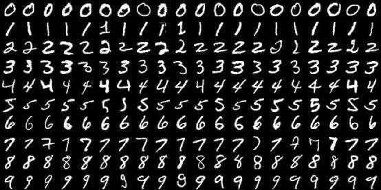
Figure 1: Example of MNIST dataset

The dataset consists of a training set and a test set, where the training set contains 60,000 handwritten digital images and the digital labels corresponding to the digital images. Similarly, the test set contains a total of 10,000 handwritten digital images and digital labels corresponding to the digital images. The data set is composed of digital images from 0 to 9, each of which is a single-channel gray scale image of 28 pixels by 28 pixels, and each pixel is a uint 8 data type, i.e., an 8-bit unsigned integer with a value between 0 and 255. Each image is labeled with “1”, “3”, “5”, etc.

6.2 Experimental Setup

6.2.1 Data Pre-Processing

The experimental dataset is a MNIST dataset. In the experimental preprocessing stage, we need to regularize and expand the images in one dimension so that when we use batch processing, we can transform a batch of digital image samples into a two-dimensional array for computation. At the same time, we encode the data labels as one-hot. One-hot encoding is an array where the correct solution label is 1 and all others are 0. For example, like label ‘7’ in one-hot encoding array is 0, 0, 0, 0, 0, 0, 0, 0, 0, 1, 0, 0.

6.2.2 Network Structure

All program networks are structured as 728 × 40 × 10, the input layer is 728 neurons with input function only, the implicit layer is 40 neurons containing the Relu function, and the output layer is a Softmax-with-Loss layer with 10 neurons. In the output layer we use a Softmax-with-Loss layer for learning.

6.2.3 Experimental Basis

The algorithm is done by Python3.6, for the implementation of the algorithm for the structure in [15,17] is consulted. The device used in this paper is CPU: Inter(R) Core(TM) i5-7500 CPU@3.40 GHz with 16.00 GB of RAM.

The experiment consists of two parts in total. The first part is mainly the evaluation comparison between the algorithm of this paper and the current mainstream algorithm; the second part is mainly the exploration of the relationship between the parameters of the algorithm of this paper.

6.3 Algorithm Comparison

The N-SVRG algorithm is programmed in PyCharm using Python3.6, and is compared with the mainstream Mini-Batch SGD, AdaGrad, RMSProp, SVRG and SCSG algorithms.

Parameter setting of each algorithm: Mini-Batch SGD:

Maximum number of iterations 4800, per batch size 250;

AdaGrad: 4800 iterations maximum, 250 per batch size;

RMSProp: 4800 iterations maximum, 250 per batch size;

SVRG: Maximum epoch count 20 times, SGD steps 5000;

SCSG: Maximum number of iterations 4800, batch size 250, number of SGD steps 250;

N-SVRG: Maximum number of iterations 4800, batch size 250, number of SGD steps 249.

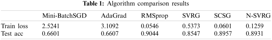
The following points can be seen in Fig. 2 and Table 1:

(1) N-SVRG, RMSProp and SCSG all reach around 65% accuracy by the first epoch of iteration, while SVRG, Mini-Batch SGD and AdaGrad only reach below 40%. As the iteration proceeds, N-SVRG, RMSProp and SCSG reach 80% or more accuracy after only 7 epochs, SVRG reaches 65%, and Mini-Batch SGD and AdaGrad reach only 50%. Batch SGD and AdaGrad.

(2) N-SVRG, RMSProp and SCSG all achieve high accuracy smoothly and quickly. In terms of accuracy, the difference between N-SVRG and SCSG is 0.26%, and the difference between RMSProp and SCSG is 1.13%. The detection accuracy of SVRG is slightly lower than the previous three algorithms, but it is still better than Mini-Batch SGD and AdaGrad.

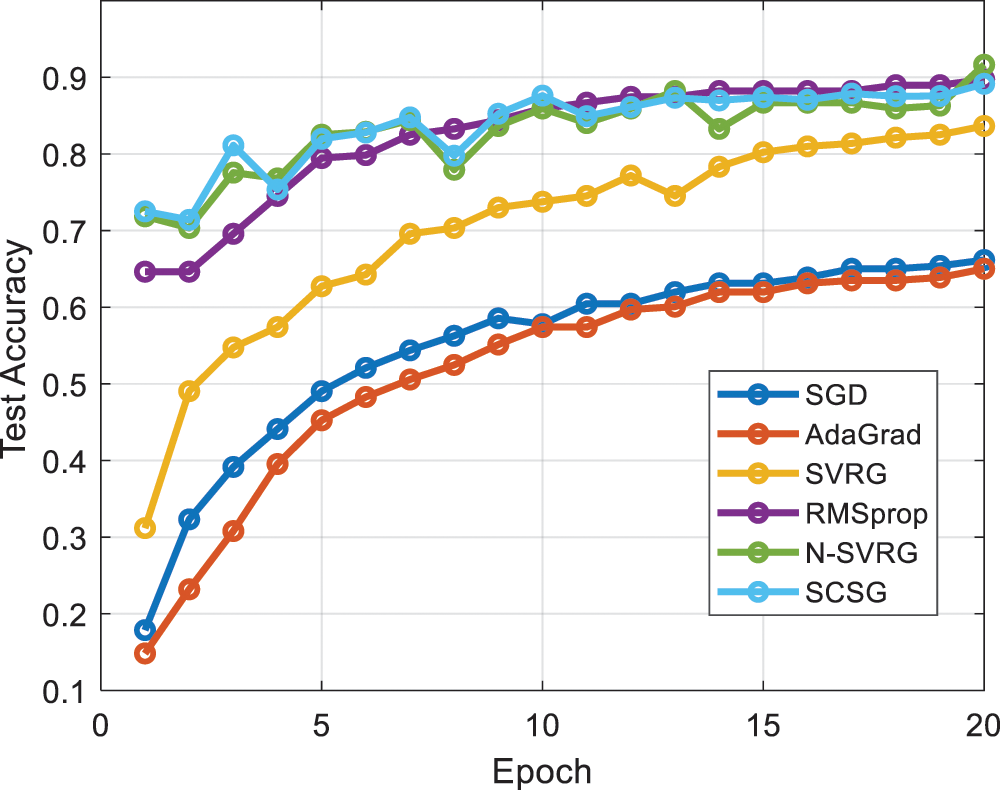
Figure 2: Comparison of algorithm accuracy

6.4 Stability Exploration

The stability of the N-SVRG algorithm is mainly affected by two factors: the size of each batch B and the number of SGD steps k. The size of B directly affects the computational cost and storage cost of the algorithm, while an appropriate B can enable the algorithm to achieve better accuracy while converging quickly, and the number of SGD steps k has a similar effect with B. Also, the size relationship between k and B is what we need to discuss. Inspired by [24], this paper focuses on two aspects of the experimental investigation, namely, the relationship between the number of training samples B and n ratio and the relationship between B and k the ratio.

B and n ratio exploration:

In the experiment to explore the effect of B and n scaling relationship on the algorithm, in order to make the experimental sample size diversity, we need to take 10,000, 8,000, 4,000 samples from MNIST data one by one for training and B ∈ n/2, n/4, n/8, n/16, n/32, set k = B − 1 for the experiment.

The following can be seen from Fig. 3 and Table 2:

(1) The proportional relationship between B and n has a certain relationship with the effect of the algorithm, the larger B is the smaller the training accuracy, and the longer the training time will be because of the number of substitutions due to the setting of k;

(2) Relatively best accuracy at B=n8 and B=n32;

(3) Although it can be seen from the detection accuracy that the size of B has a relationship with the convergence speed and the accuracy of the algorithm, especially B=n2 and B=n4, it has less impact on the stability of the algorithm and still obtains relatively good results with a simple network structure and strong robustness.

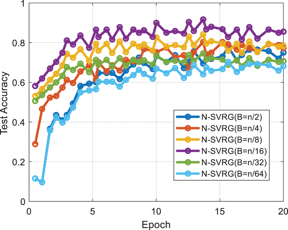
Figure 3: Results of the B vs. n ratio investigation

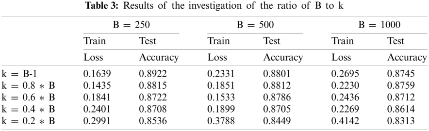
In the experiments exploring the effect of the relationship between B and k scaling on the algorithm, we directly use the complete MNIST dataset and consistently sample small batches of samples of sizes 250, 500, and 1000, respectively. while we set the number of SGD steps k ∈ B-1, 0.8 × B 0.6 × B 0.4 × B 0.2 × B for the experiments.

The following can be seen in Fig. 4 and Table 3:

(1) The relationship between the size of k and B is positively related to the accuracy of the algorithm, the closer k is to B, the higher the testing accuracy of the algorithm, and vice versa, the accuracy decreases, and this phenomenon does not change with the size of B.

(2) From the cross-observation of the data, it is clear that when k is a constant (k = 200), the accuracy decreases with the increase of B, which confirms the above point.

(3) Comparing the results of two experiments, Experiment B with n-proportional probe and Experiment B with k-proportional probe, we can see that the N-SVRG algorithm is robust and maintains high experimental results for general optimization problems when the batch size is too small.

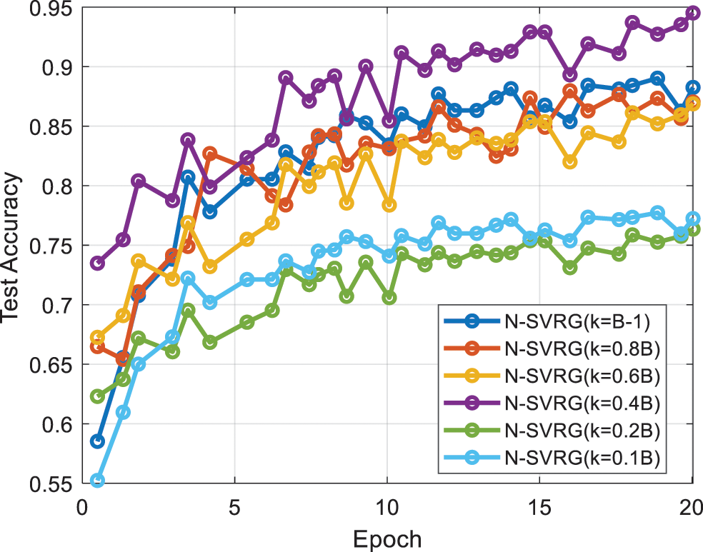
Figure 4: Results of the B vs. k ratio exploration

6.5 Discussion

Through the experiments we can find that the N-SVRG algorithm is outstanding in convergence speed and accuracy compared with Mini-Batch SGD, AdaGrad and SVRG, and is comparable to RMSProp and SCSG. We can know that N-SVRG algorithm is a relatively stable algorithm, although there are two parameters B and k affect the accuracy of the algorithm, from the experiment we can see that the change of B shows a trend of the smaller the value, the higher the accuracy of the algorithm, this nature is the algorithm is suitable for general optimization problems.

7  Conclusion

In this paper, we propose a noise reduction method for SVRG, which uses a small batch of samples instead of all samples for average gradient computation and incremental update of the average gradient. The experiments are compared with the mainstream Mini-Batch SGD, AdaGrad, RMSProp, SVRG and SCSG algorithms, and it is proved that the N-SVRG algorithm outperforms SVRG and SASG, and is equal to SCSG. Finally, by exploring the relationship between the small values of different parameters n, B and k and the algorithm effect, we prove that the N-SVRG algorithm has some stability.

Funding Statement: This work was supported by the National Natural Science Foundation of China under Grant 62076066.

Conflicts of Interest: The authors declare that they have no conflicts of interest to report regarding the present study.