Computer Modeling in Engineering & Sciences

DOI: 10.32604/cmes.2022.019112

ARTICLE

A Flux Based Approximation to Simulate Coupled Hydromechanical Problems for Mines with Heterogeneous Rock Types Using the Material Point Method

Gysbert Basson*,1 andrew P. Bassom2, and Brian Salmon3,*

1Institute of Mine Seismology and University of Tasmania, Kingston, 7050, Australia
2School of Natural Sciences–University of Tasmania, Sandy Bay, Hobart, 7001, Australia
3School of Engineering–University of Tasmania, Sandy Bay, Hobart, 7001, Australia
*Corresponding Authors: Gysbert Basson. Email: Gys.Basson@IMSeismology.org
Received: 03 September 2021; Accepted: 21 October 2021

1  Introduction

Numerical modelling is an essential tool for understanding the induced stress changes in underground hard rock mines. Mines rely on these tools for numerous purposes, of which arguably the most important is the planning of mining operations that mitigate seismic risk. Since engineers cannot physically observe the solid rock mass, numerical techniques must be capable of providing reliable predictions of the complex behaviour of the material. Many of the available commercial software packages simulate models that only allow for a single solid phase and frequently neglect groundwater’s influence on the stress regime in the rock mass [1–4]. Studies investigating the effect of groundwater principally concentrate on mine dewatering or the environmental impact in coal mines [5–8]. The coupled effect of the pore water pressure on the stress in the solid of hard rock mines is often overlooked when undertaking numerical stress modelling experiments. For example, it is expected that the effective stress of rock decreases as the water pore pressure increases. Therefore, it means that a geological fault that is filled with water may become unclamped under high pore pressure, making it much more likely to slip and consequently more seismically hazardous. Experiments that exclude the effect of the fluid may misleadingly suggest that the fault is stable. It is this prospect that motivates much of the work in this paper, in which we present a new numerical tool to aid hard rock mining applications which takes explicit account of the fluid phase, and thus making our tool a multiphase solver. We emphasize that we use the term multiphase to refer to the solid and fluid phases of the different materials in our context. This contrasts with the term multiphase’s standard meaning in petroleum engineering, where it is typically used when discussing two different fluids such as oil and water.

A standard modelling technique that is often used in the mining industry is based on boundary elements. The Boundary Element Method (BEM) [9] can represent large-scale mining configurations but assumes a medium that is linear elastic. This restricts its use to heterogeneous rock situations, making it less suited to the simulation of more complex multiphase problems. On the other hand, Finite Element Method (FEM) based solvers tend to be very reliable for analysing a wide range of mining-related problems. It has the distinct advantage that it can be used to model complex mining geometries in heterogeneous mediums. Furthermore, many extensions of the basic FEM, like the control volume FEM (CVFEM) [10], can simulate the coupled effect of multiphase problems. However, FEM can struggle when handling large deformations, and complex remeshing techniques are often essential to deal satisfactorily with this effect. To alleviate this problem, we suggest and investigate the properties of another family of methods often referred to as the Material Point Method (MPM) [11]. This strategy is attractive because the MPM can describe large deformations without invoking expensive and intricate remeshing. In mining simulations, grid locations near excavations (empty spaces) are susceptible to undergoing large deformations if high stresses exist. Moreover, the MPM can construct layouts with complex geometries with relatively little effort; this property is a direct consequence of the fact that the technique relies on a regular grid and so avoids the remeshing complications typically encountered within FEM. Furthermore, it has the property that it can simulate coupled multiphase problems using a single solver, therefore by-passing the need for a hybrid approach. One drawback of the MPM is its computational cost since particle, as well as grid states, have to be accounted for. High-density grids of entire mining layouts may necessitate significant memory resources. Basson et al. [12] describe a way to alleviate this effect by making use of a layered MPM background grid to simulate large mining problems.

The original formulation MPM was proposed by Sulsky et al. [11]. It is a hybrid Lagrangian and Eulerian Particle-In-Cell method that uses Lagrangian material points (otherwise known as particles) to carry history-dependent properties and employs an Eulerian background mesh as a communication tool for transferring information between the particles. Physical properties are first interpolated onto the background mesh, then the equations of motion are solved, and finally, the updated states are interpolated back to the particles themselves.

The MPM has been successfully used to study many problems, and its application to geotechnical questions [13–15]. More recently, the MPM has been extended to account for multiphase problems that embody fully coupled soil-fluid interaction [16–19]. The treatment of multiple phases within hydro-mechanical geotechnical problems using a single solver is particularly interesting to our current study. This method, used in the investigations [20,21], eliminates the need for complicated hybrid approaches that would otherwise be necessary to handle the coupling of the various phases.

Many coupled MPM formulations use the Biot theory approach [22] in which the momentum balance equation for the solid phase is solved on the Eulerian grid, and a Darcy velocity is assumed to describe the relative motion of the fluid with respect to the solid. The theory of mixtures [23] has also been successfully applied; this approach is founded on momentum balance equations solved independently on the Eulerian grid, while the coupling is modelled by introducing drag terms for both phases. Bandara [24] has successfully applied both the theory of mixtures and the Biot’s theory approach and used a two-point formulation to describe the coupled MPM (see Fig. 1). In the two-point formulations of the multiphase MPM, the medium consists of distinct groups of particles for each phase; solid particles and fluid particles are treated separately. This leads to the doubling up of particles within the grid and requires extensive computational resources. In the single-point formulation of the MPM, each particle carries information about both phases simultaneously.

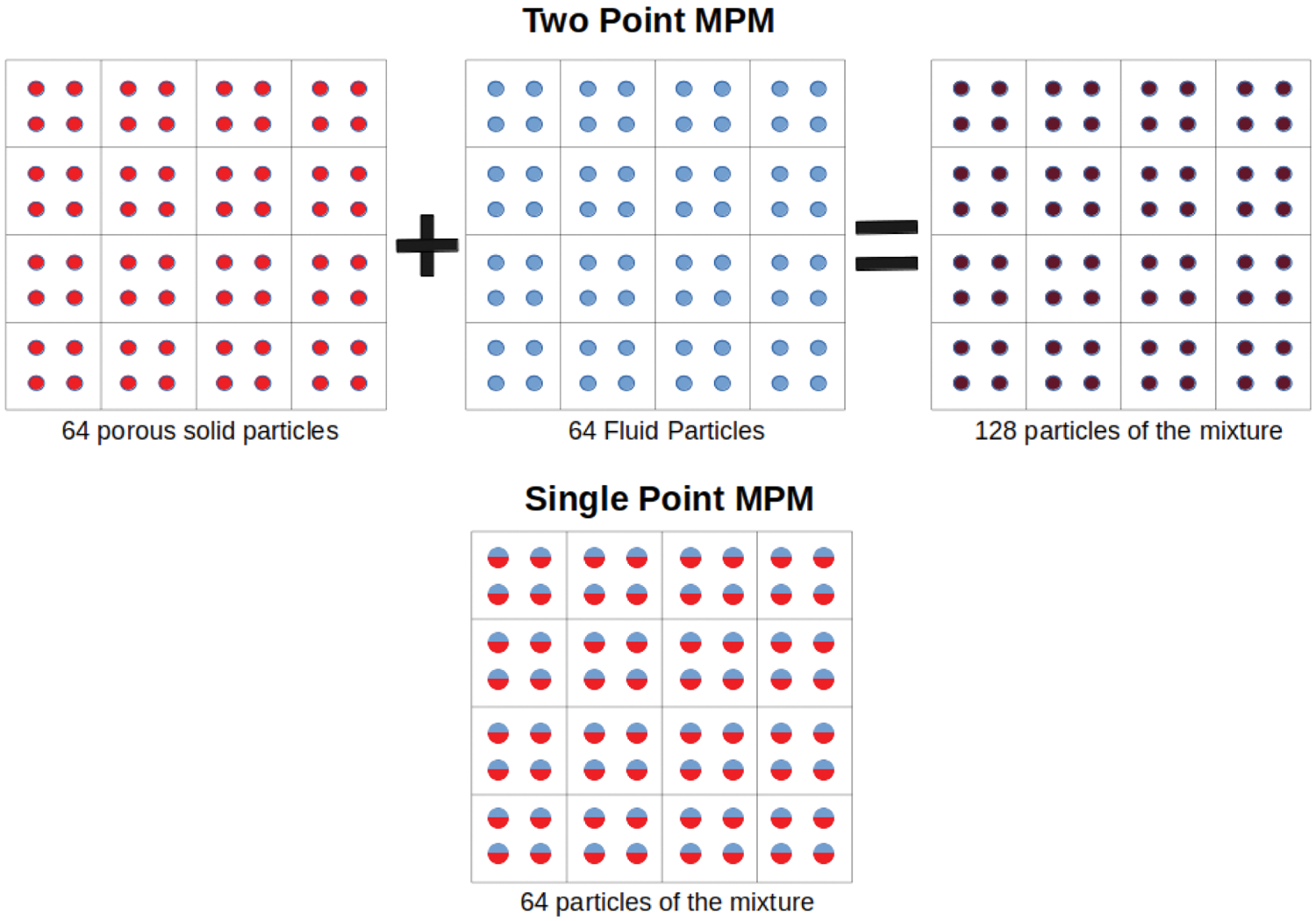
Figure 1: An illustration of the difference between the single-point and two-point implementations of the two-phase MPM. Top: the mixture is represented by a total of 64 porous particles representing the solid phase and another 64 fluid particles for the fluid phase giving 128 particles in total. Bottom: now, the mixture is represented by 64 particles, each of which carries information about the states of both phases

Both Al-Kafaji [16] and Bandara et al. [17] have used a single-point formulation to solve problems within saturated porous media. Yerro et al. [19] extended the single-point formulation to allow for three phases in which solid, fluid and gas components are coupled. Each formulation has its advantages and disadvantages, and arguably none are demonstrably superior to the others in all instances. Instead, the choice of the particular implementation is best guided by the details of the specific problem at hand. For example, when a problem requires the presence of free water (see Fig. 2 as well as pore water, then the use of a two-point formulation based on Mixture Theory is recommended. However, attempting to apply this to quasi-static problems requires additional mechanical damping to both phases simultaneously, which may be difficult as this could lead to pressure oscillations [24]. It significantly increases the computational overhead associated with the requirement to account for both solid and fluid particles. If there is no free water present, then it is much easier to implement a single-point formulation as the position of the fluid is redundant and focus can be directed on the fluid pressure and velocities at the location of the solid particle instead. Therefore, for our study, the single-point MPM was chosen since our interest is to assess the response of the solid phase due to pore pressure changes in the fluid. Our investigations do not require any free water, which is ignored henceforth.

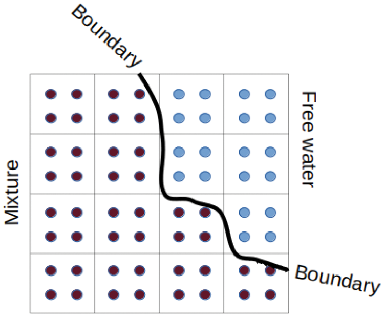
Figure 2: An example of the two point implementation of the MPM to represent a fluid-solid mixture together with free water particles lying outside the boundary of the mixture

The remainder of the paper is structured as follows. In Section 2 we first outline the problems associated with using existing coupled MPM approaches to simulate materials with heterogeneous permeability. We then propose a modification that enables MPM to cater for mediums with variable permeability; this is the subject of Section 2.1. We then describe the details of a full computational cycle of our modified MPM. The performance of our new method is validated in Section 3 against two well-known analytical expressions and a comparison with the performance of a conventional coupled MPM as commonly found in the literature. Having benchmarked the new method against some test examples, we then use it to model an actual active mine in Section 4; in particular, we investigate the effect of pore pressure changes of a fluid-filled fault on the surrounding stress. We conclude the paper with some observations and final remarks.

2  Problem Description

In a single-point formulation of the two-phase MPM, the medium is represented by a solitary particle layer which means that each particle must carry information about both the solid and fluid phases. Most existing literature that uses this approach assumes that the continuum is defined as a homogeneous porous solid material with constant permeability and porosity [16,17,24]. This can be problematic when trying to simulate heterogeneous materials in which the permeability is heterogeneous. It is essential for what follows, so it is worth exploring this claim a little further. The schematic shown in Fig. 3, sets out, in simple terms, the main elements needed to advance the coupled MPM through one time step. For definiteness, let us suppose that the background grid is a regular Cartesian mesh; we need to bear in mind that what happens in this instance equally applies to more intricate nonstructured grids. The grid is initially populated with particles in some predetermined state, as depicted in Fig. 3a. The particle properties are then mapped onto the nearby cell nodes; this interpolation is performed using suitably chosen shape functions (Fig. 3b). In the original formulation of MPM, the shape functions are standard tri-linear forms similar to those often used in FEM methods. In more advanced versions of the implementation, higher-order shape functions can be used if greater transfer tiers are required outside the host cell (see, for example [25], or a variant of the MPM known as the Generalized Interpolated Material Point Method (GIMP) [26]). This intentionally smears information over a much larger volume than the cell occupied by the particle; this is a complicating factor when simulating nonhomogeneous materials as usually a clear boundary between different materials cannot be distinguished. Several adaptions that purport to address this problem in the MPM have been proposed [27–30]. In Fig. 3c, the grid is stepped forward in time by solving the equations of motion at the grid nodes. Once complete, the particles are updated in Fig. 3d. These include position, velocity and stress, among others. Finally, in Fig. 3e, the grid is reset in preparation for the next time step.

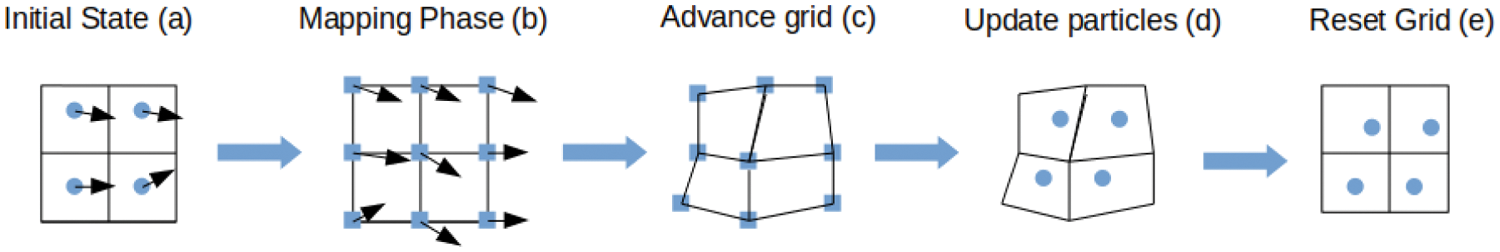
Figure 3: A flow diagram illustrating the stages required to advance the coupled MPM through one time step

To delve a little deeper into the source of the problem, we focus on the process by which the fluid phase properties are mapped onto the nearby nodes, see Fig. 3b. First, we define the generalised Darcy’s law [31–33] for a fluid phase α according to

wα=−κgρα(∇pα+ρα(g−as)), (1)

where wα is the relative velocity of the fluid to the solid phase; κ is the solid phase conductivity (units m/s); pα is the fluid pore pressure; ρα is the fluid density; g is scalar gravity; and g and as denote the gravitational acceleration and the acceleration of the solid phase, respectively. The fluid velocity at a node of the background mesh can be discretised to (as explained in detail in [34])

wα=κMg(∑Np∇S(x)pαVα)+κ(g−as)g. (2)

The summation is taken over all Np particles that are located in the cells that share this node and depends upon the gradient of the shape functions S(x). In this expression, Vα represents the fluid phase volume of the particle determined using

Vα=nVp (3)

where n is the solid phase porosity and Vp is the combined particle volume of both the solid and fluid phases (see Section 2.2 below for more detail on the particle volume calculation.) Furthermore, the fluid phase mass of an individual particle is

mα=Vαρα (4)

so that the total nodal fluid phase mass is expressed as M=∑NS(x)mα. When a material is isotropic, and κ is uniform, Eq. (2) correctly calculates the nodal Darcy velocities as illustrated in Fig. 4.

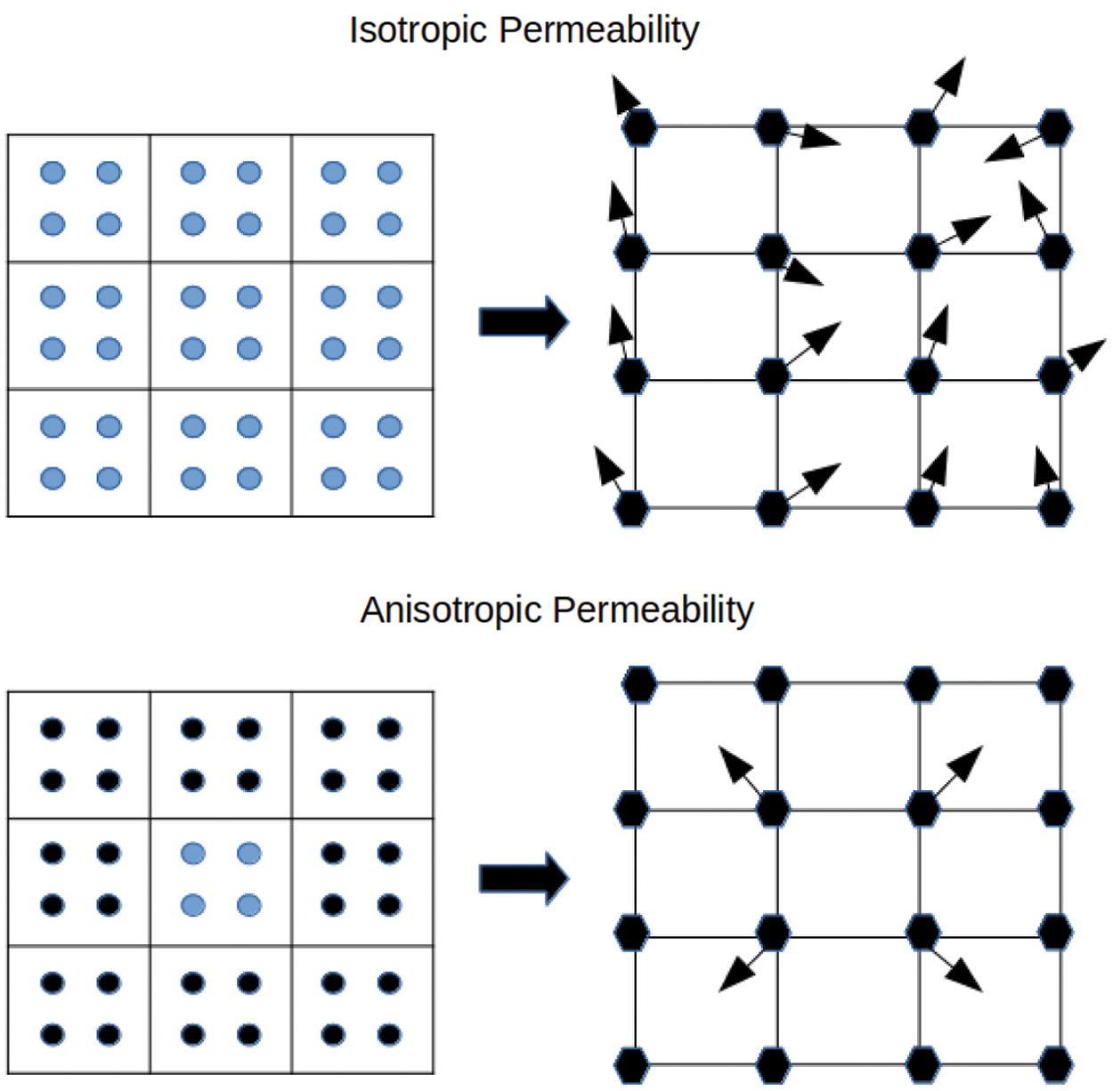
Figure 4: The effect of an heterogeneous material on the predicted fluid velocities. We show in the upper diagram the situation that arises when the material in which all particles have the same permeability. The fluid phase velocities (arrows) calculated at the grid nodes are correctly resolved by standard MPM techniques. To contrast the situation when there is non-constant permeability, consider the material in the lower diagram; here it is supposed that the cell containing blue particles has one value of permeability while the surrounding cells with black particles all have zero permeability. In this scenario, standard MPM interpolation techniques will predict an incorrect fluid phase velocity at the four interior grid nodes where the velocity should be zero

On the other hand, when the material is heterogeneous, the situation changes as κ is no longer constant around the node. To amplify this point, assume the cell at the centre of the grid contains particles for which κ is non-zero but that κ=0 in the neighbouring cells as sketched in Fig. 4 We would expect wα=0 at these nodes of the central cell as no fluid can be passed from this cell to its neighbours. However, if we naively apply Eq. (2) we note that wα is non-zero, ultimately resulting in a loss of pore pressure in the particles of the centre cell. We need to address this issue to ensure that mediums with heterogeneous permeability can be modelled faithfully.

2.1 Application of the Two Point Flux Approximation within the MPM

When using domain discretisation approaches to solve partial differential equations, a relatively large domain is divided into smaller elements, otherwise known as finite volumes (FVs). Finite Volume methods are usually the industry-preferred method for solving problems involving porous media as they are based on the conservation of continuity of fluxes [35]. These methods can be divided into two main classes, namely Two Point Flux Approximations (TPFA) [36] and Multi Point Flux Approximations (MPFA) [37]. TFPA methods are widely used in commercial software packages to study fluid flow in porous media; it is an attractive approach because it is simple to implement and computationally efficient. However, these methods struggle to accurately resolve the flux for grids that are not K-orthogonal; that is, instances when the principal directions of the permeability tensor do not coincide with the orientation of the input grid. The standard TPFA must be adapted to deal with such cases [38]. On the other hand, MPFA methods are adept at solving problems involving unstructured grids. Furthermore, as mentioned previously, when dealing with the full permeability tensor, one may choose to solve the problem using either FEM, Mimetic Finite Difference or the MPFA [39]. However, these implementations are typically much more complicated than the TPFA, which leads to a computationally expensive algorithm. In what follows, we attempt to adapt the TPFA to fit into the computational scheme of the MPM, and since the standard MPM grid is K-orthogonal, it follows that the TPFA is the preferred choice. If, however, unstructured grids are to be considered, then the MPFA should be preferred.

The total fluid flux through the surface of a finite volume can be written as

F=−∫Ω(K∇pα)⋅ndΩ (5)

where n is the unit normal vector on the boundary of a surface dΩ that points away from the centre of the cell; and K is the full permeability tensor. Within the MPM framework, the background grid cells can be considered as finite volumes. Thus, if the cell C is a three-dimensional cube, then this is formula is adapted so that

FC=−∑∫Ω(K∇pα)⋅ndΩ (6)

where the sum is taken over the six faces of the cube. The integral term on the right-hand side of Eq. (6) is usually referred to as the flux through face dΩ. If this depends only on the scalar pressure across the edges of the cell, then the discretisation method is of TPFA type, but if the fluid pressures of surrounding cells also enter the integral, we are dealing with a MPFA case. We will assume the pressure varies linearly across two adjacent cells for our calculations, and thus we follow the TPFA approach.

To demonstrate how the flux at the interface of two cells are calculated in practice, consider two cells A and B, each with length l, as depicted in Fig. 5. Suppose that cell A has permeability k1, cell B has permeability k2 and that the shared face q of the two cells is a distance l/2 from the centre of each cell. The flux between the centre of A and q can be written

FA|q=k1pq−pAl/2 (7)

where pq is the fluid pressure at the interface and pA is the fluid pressure at the centre of A. An analogous expression for the other cell gives

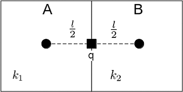
Figure 5: A schematic of a one-dimensional application of the TPFA. Here we have neighbouring cells A and B, each of side l, but with different permeabilities k1 and k2. The purpose of the TPFA is to calculate the flux across the common face q

FB|q=k2pq−pBl/2 (8)

where pB is the fluid pressure at the centre of B. Since the fluxes FA∣q and FB|q should be the same, this enables us to deduce that

pq=T1pA+T2pBT1+T2 (9)

where Tj = kj/l with j = 1, 2. If we use Eq. (9) in expression (7) we obtain the flux expression

FA|q=21/T1+1/T2(pA−pB), (10)

which shows that the flux through q is a function of the harmonic average of the permeabilities of the two cells. If we were to apply Eq. (10) directly within the MPM framework, we would need to conduct additional calculations to determine the flux across all the cell interfaces in the background grid. Although the MPM scheme can be modified to include this step, it is undesirable as it adds extra computational overhead to the algorithm. Furthermore, since the nodes of the background mesh are used directly in the method, it would be advantageous to resolve the Darcy velocities at the nodes of the background mesh rather than across the interfaces of the grid cells. A schematic of conventional mapping scheme is depicted in Fig. 6 and requires the direct application of Eq. (2) to each one of the nodes denoted by the black squares. The Darcy velocity depends on the pore pressure and conductivity of all particles in the cells that share the node. As already mentioned, this method is only accurate if the conductivity of the particles contributing to the node is isotropic.

To improve matters, here we propose a modification of Eq. (2) to ensure that each node only uses information gleaned from particles located in cells that share a common interface. This will allow fluid flow to only occur across these boundaries, as is the case in the TPFA. To explain the process, we direct the reader to the second diagram in Fig. 6. Here we have drawn nine square cells, with the central one denoted C. Now the goal is to set the Darcy velocities at each of the four nodes of C such that it describes the total fluid flux through the surfaces of C. For definiteness, let us focus on the upper-left (north-west) node of C, which we have labelled Q; this choice of the node is not essential, and analogous considerations apply for the other three nodes of C.

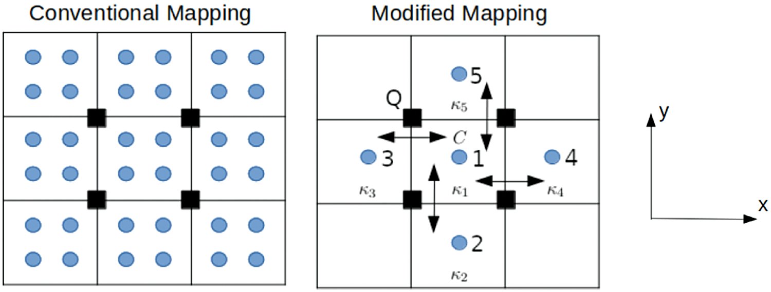
Figure 6: An illustration of the distinction between the conventional mapping technique employed in MPM and the modification suggested in the current work. In the left-hand diagram, which relates to the conventional approach, Eq. (2) is applied to all particles (indicated blue) in the grid. The Darcy velocity at a particular node (black rectangles) is inferred from the velocities of all the particles within the cells which share the node. The Darcy velocity at the node can point in any direction as a result of the particle summation. Right: particle pore pressures are combined to obtain a cell centered average pore pressure. Fluid flow is then limited to cells that share common faces with each node

We base many of our design decisions guided by the strategy employed in the usual TPFA. First, we remark that in examining node Q, we will only consider contributions from particles located in cells 1, 3 and 5; that is, cell C together with those cells that have Q has a node and which share an interface with C (i.e., the cells to the north and the west of C). For each of these, the cell pore pressure pc is set to be the average value of the individual particle pressures so that

pc=1Np∑Nppα, (11)

where Np denotes the number of particles contained in the cell and pα is the particle pore pressure. The fluid mass mc in each cell c is calculated from Eq. (4) as mc=nVcρα where Vc is the volume of the cell. The total fluid can then be mapped to Q and becomes

MQ=∑NcS(xc)mc (12)

where S(xc) is the shape function evaluated at the position of the centre of the cell and Nc is the number of cells (in our example case three).

The standard shape functions of an isoparametric hexahedron can be calculated using the schematic idea that is sketched in Fig. 7. The illustration shows how to compute the shape function for a one-dimensional problem, and this is then easily extended to three dimensions by calculating the product of three one-dimensional functions S(x)=S(x)S(y)S(z). The sides in Fig. 7 are simple linear functions that ensure that the weighting varies from 1 if the point x lies on the node and zero if it coincides with a neighbouring node.

Next, the conductivity term is evaluated independently for each cell that shares an interface with C and has Q as one of its nodes. In this example, there are two such cells, and we denote these interfaces c1∣3 and c1∣5. We have previously seen that the conductivities at the interfaces are simply the harmonic average of the relevant two cell conductivities so can be expressed

κ1|3=21/κ1+1/κ3 and κ1|5=21/κ1+1/κ5. (13)

Figure 7: A schematic of a one-dimensional linear shape function that is commonly used in the MPM. In three dimensions the shape function can be calculated using S(x)=S(x)S(y)S(z)

With these key changes in mind, we can now derive the appropriately modified version of Eq. (2). To start the process, it is convenient to imagine that κ is uniform around Q (although we relax this in due course). Applying Eq. (2) directly to Q as done in existing MPM approaches gives

wQ=κMQg{∇S(x1)p1V1+∇S(x3)p3V3+∇S(x5)p5V5}+κ(g−aQ)g (14)

where the terms Vi, pi and ∇S(xi) denote the fluid volume of cell i and the pressure and the gradient of the shape functions evaluated at the centre of that cell. In the last term aQ represents the nodal acceleration of the solid phase at Q; we say more about calculation of this quantity in Section 2.2 below. Note that there is no restriction on the direction of the fluid flux in Eq. (14) and requiring the flux to be only perpendicular to the boundaries of c1∣3 and c1∣5 require a modification to the formulation.

As has been kindly pointed out to us by an anonymous referee, if κ is just a constant scalar, expression (14) simplifies to Eq. (2) and then the procedure becomes similar to that typical in a standard two-phase implementation. However, in our TPFA approach, the aim is to define a relation that is dependent only on the adjacent neighbours around node Q of cell c in Fig. 6. We see that cell 1 contributes to Q through both the interfaces, c1∣3 and c1∣5, whereas cells 3 and 5 contribute to Q only via c1∣3 and c1∣5, respectively. Furthermore, since κ is no longer constant, its value needs to be ascribed correctly depending on which interface is relevant.

With these changes taken into account we can modify (14) to

wQ=VMQg{∇S(x1)⊙n1|3p1κ1|3+∇S(x1)⊙n1|5p1κ1|5+∇S(x3)⊙n1|3p3κ1|3+∇S(x5)⊙n1|5p5κ1|5}+1g{S(x1|3)κ1|3(g−a1|3)+S(x1|5)κ1|5(g−a1|5)} (15)

where n1∣3 and n1∣5 denote the normal directions of the interfaces c1∣3 and c1∣5, the symbol ⊙ represents the element-wise product of vectors and a1∣3 and a1∣5 represents the acceleration of the solid phase of respective interfaces. These are simply taken as the average value of the acceleration of the interface nodes. The terms S(x1∣3) and S(x1∣5) represent shape function values evaluated at the interface centre position. In our example we can simplify matters somewhat because our cells are of equal volumes V. Since the shape function gradients are evaluated at the respective cell centres, it follows that ∇S(x1)⊙n1∣3=−∇S(x3)⊙n1∣3 and ∇S(x1)⊙n1∣5=−∇S(x5)⊙n1∣5. With this, Eq. (5) becomes

wQ=VMQg{∇S(x1)⊙n1|3κ1|3(p1−p3)+∇S(x1)⊙n1|5κ1|5(p1−p5)}+1g{S(x1|3)κ1|3(g−a1|3)+S(x1|5)κ1|5(g−a1|5)}. (16)

We have developed result (16) with the specific node Q in mind. However, this balance can easily to extended so as to apply for any of the nodes of cell X: specifically

w=VCMg{∑c∇S(xC)⊙nC|cκC|c(pC−pc)}+1g∑cS(xC|c)κC|c(g−aC|c) (17)

where subscript C represents a value evaluated at cell C and subscript c represents a value evaluated at an adjacent cell that shares a common interface with C as well the the node.

Given this modified expression for the Darcy velocity, we need to embed it within the cycle of calculations that are required to complete a time step within the modified MPM.

2.2 The MPM Method

In this section, we will explain how we deploy the dynamic MPM in our modelling experiments. The Lagrangian particle layer present in our solid skeleton and the momentum balance equations for the fluid-solid mixture are solved on a regular Eulerian background mesh composed of trilinear shape functions S(x). Isothermal conditions hold as we shall assume that there is no mass exchange between phases, the solids are always fully saturated, and there is no acceleration of the fluid with respect to the solid. Moreover, we suppose that the densities of the two phases remain constant, the porosity of the solid phase does not change, the compressive stress is negative, while the pore pressure is positive.

Our medium is heterogeneous, which means we can not assume constant conductivity as commonly adopted in the majority of MPM applications [16,17,24]. We, therefore, need to carefully consider our treatment for determining the Darcy velocity of the fluid phase at the nodes of the background grid in the presence of this complication.

To initiate our model, suppose that at time t a particular particle p is positioned at xpt, has velocity vpt and occupies a volume Vp0. We assume that the Cauchy effective stress is σpt and the strain is εpt (both expressed in Voigt notation). Furthermore, the solid phase conductivity κp0, the fluid pore pressure ppt together with the solid phase mass ms=(1−np)ρsVp0, in which ρs is the solid phase density and np the particle porosity, are all known.

With this particle state specified, we can derive:

1. the volume of the mixture Vpt=(1+ε1pt)(1+ε2pt)(1+ε3pt)Vp0;

2. the fluid phase mass mα=npραVp0, where ρα is the fluid phase density and

3. the particle mass mp=ms+mf, where ms and mf denotes the mass of the solid and fluid respectively.

The method then proceeds as follows. For each particle p, we can identify the particular grid cell that contains p and then links are created between p and the eight nodes of that cell. Reciprocal links from the nodes back to the particle are formed, and the combined information is stored in a bi-directional map Ml↔p which is called upon all subsequent steps whenever interpolation is required.

For each grid node l, we use the information within Ml↔p to identify all the associated linked particles. These having been found, we can compute the mass mlt, and velocity vl of the node using

mlt=∑p=1NpmpS(xpt)andvl=∑p=1NpmpvptmltS(xpt) (18)

respectively. The force exerted due to the solid-fluid mixture is

flt=∑p=1Np[−∇S(xpt)(σpt−pptq)Vpt+(mpb+ts)S(xpt)] (19)

where q = [1 1 1 0 0 0]T, b is a body force (such as gravity) acting on the particle p, and ts is an external traction force acting on the solid phase of the particle. The linear momentum balance equation for the mixture is solved at the node using

alt=flt+fldmlt, (20)

where the frequency independent damping term is defined to be

fid=−γ|flt|sign(vlt) (21)

and is added to enhance the numerical stability of the process and to encourage the convergence to a quasi-static solution [40]. The constant γ is a dimensionless damping factor, and empirical evidence suggests it should typically be set somewhere in the range 0.7–0.85, see, for example, [15]. The nodal velocity at the end of the Lagrangian step is updated using Eq. (20) so that

vlt+△t=vlt+alt△t (22)

and boundary conditions for alt and vlt+△t can be applied if necessary.

At this point in the process, our novel MPM formulation deviates from many of the established two-phase MPM strategies. In these standard versions, the nodal Darcy velocities are calculated by appealing to Eq. (2), but, as we have already discussed, this does not take into account any anisotropy in the conductivity of particles. We have shown that Eq. (17) captures this phenomenon, and we use this balance to execute nodal Darcy velocity calculations.

Having updated the state of each node, we can revert to the particles. For each particle, we use Ml↔p to identify all the nearby grid nodes Nn within its range and use them to calculate several relevant quantities. First, we update the position and velocity of the particle using

xpt+△t=xpt+△t∑l=1Nnvlt+△tS(xpt)andvpt+△t=vpt+△t∑l=1NnaltS(xpt) (23)

while the strain increments for the solid phase are

ε˙s=△t2∑l=1Nn[∇S(xpt)vlt+△t+(∇S(xpt)vlt+△t)T]. (24)

The fluid phase strain increment for each particle requires the calculation of the average pore pressure and conductivity of the cell which are set to be

pct=1Np∑p=1Nppptandκct=1Np∑p=1Npκpt. (25)

Each cell is then revisited to deduce the associated nodal Darcy velocities wlt for the nodes only belonging to that cell. This is done by applying Eq. (17) to each face of the cell in turn. As an aside, we need to emphasise that once wlt is calculated for all the nodes of a specific cell; these are then cleared before the algorithm proceeds. Otherwise, should a particular node lie on the boundary of two or more cells, when evaluating Eq. (17) for the second (or subsequent) cell, a previous value of wlt stored from an earlier calculation may contaminate the analysis. Once all the values for wlt known for all nodes, we can compute the particle fluid phase strain increment using the standard expression

ε˙α=△t2∑l=1Nn[∇S(xpt)wlt+△t+(∇S(xpt)wlt+△t)T] (26)

and the pore pressure is advanced using

ppt+△t=ppt−△t(Kfnp)(tr(ε˙α)+tr(ε˙s)) (27)

where Kf is the fluid bulk modulus. The appropriate constitutive relation can then be applied to update the particle stress. Once all particle information has been advanced, the whole system has been moved through one timestep, and the process can then be repeated.

2.3 Time Step Scaling

The explicit nature of the proposed iteration scheme means that the timestep △t must be chosen sufficiently small that the usual Courant-Friedrichs-Levy (CFL) [41] condition holds and stability of the solution method is ensured. An upper bound on the proper time step is given by △tc=L/vp, where L is the smallest cell length of the background grid and vp is the velocity of the pressure wave for the applied material properties. For mining-related studies, the value of △tc typically lies in the range from 1×10−7 to 1×10−4 seconds. Such small values can be problematic when simulating coupled pore pressure diffusion problems, as typically one would need to simulate millions of time steps.

Fortunately, for a simulation that is kept near quasi-static equilibrium, this stringent constraint on the timestep can often be relaxed somewhat. Basson et al. [12] used the maximum nodal unbalanced force ratio and maximum particle velocity of the MPM to determine whether a system is in approximate equilibrium. If it is, the time step can be safely increased by adapting Eq. (20) to

alt=flt+fldmltDt, (28)

where Dt is a mass density scaling factor. Here we set Dt = 1 if model is not in equilibrium but set Dt+△t=kDt if it is. Experiments suggest that optimal performance is achieved if k≈1.005 which corresponds to a time step △t=Dt+△t△tc.

3  Benchmarking of the Method

Before using our technique in practical contexts, it is essential to validate its performance against well-known and standard examples. For this purpose, we selected two problems [24] for which analytical results exist. The case studies were specifically chosen to test our new MPM and compare it with the results of existing two-phase MPM implementations. These benchmarks assume the medium has homogeneous permeability and thus, unfortunately, will not test the performance of our method when handling heterogeneous cases since analytical expressions for these cases are very sparse. On the other hand, one of the key features of our technique is that its treatment of the fluid-phase coupling is very different to that implicit in other coupled MPM formulations. In this way, our tests compare the performance of our methodology against analytical knowledge and give a way of assessing its usefulness and advantages over existing MPM implementations. In our experiments, we examined the values of the two sums in Eq. (17)

T1=VCMg{∑c∇S(xC)⊙nC|cκC|c(pC−pc)}andT2=1g∑cS(xC|c)κC|c(g−aC|c) (29)

in the two subsections that follow.

3.1 Geostatic Stress Distribution Due to Gravity

The first example taken from Bandara [24] explores the geostatic consolidation problem presented by a fully saturated one-dimensional soil column. The initial solid-phase effective stress and fluid phase pore pressure are set to be zero at time t = 0. Gravity is then applied to the material, and the system is allowed to evolve to quasistatic equilibrium. The final solution is known to be

σT=z[(1−n)ρs+nρα]g,σs=z[(1−n)ρs+ρα(n−1)]gandpα=zραg, (30)

where σT is the total stress at depth z; σs is the effective stress of the solid phase; n is the solid phase porosity; and ρα and ρs is the density of the fluid and solid phases, respectively. Even though the value of T1 will influence the results as the system settles towards its final steady-state, this test is beneficial for monitoring T2 as the effect of gravity on the fluid phase will dominate wα at the grid nodes and consequently the final pore pressure obtained in the particles. To be more specific, since our method does not incorporate all the particles around a particular node, as is conventionally done in MPM, the nodal mass term M and cell mass terms mc feed directly into the final solution of the fluid phase pore pressure. If either of these terms is not resolved correctly, then the output of the method will differ from the known analytical expressions.

Our experiment was conducted on a grid of dimensions 0.12×0.02×1 metres. The grid was subdivided into identical cells, cubic and with side 2 cm; each cell was seeded with eight particles. The material properties used in our computations are listed in Table 1. The experimental results are depicted in Fig. 8 where we also compare our model with that Bandara [24]. Agreement with the analytical expression confirms that our modified strategy performs very well, at least for this test case.

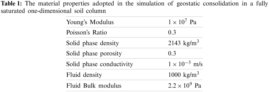
Figure 8: Predictions of the effective stress and the pore pressure as given by our modified MPM method. The agreement between the theoretical and numerical results is excellent. For comparison purposes the equivalent results obtained by Bandara [24] using a two-point coupled MPM method are shown in the right hand panel

We remark that in the course of the calculation, we noted the presence of oscillations in both the pore pressure and effective stress profiles during the system’s evolution and before settling to equilibrium. This phenomenon is illustrated in Fig. 9 and has been widely documented in literature [42,43] for other coupled methods. Further probing of the system revealed that these oscillations arise owing to the presence of the drag term aC∣c in Eq. (17). The omission of this term suppresses the oscillations, but the system still attains the final equilibrium state as predicted by the analytical expressions. While it may be acceptable to ignore the aC∣c component in those problems for which only the final quasistatic solution is of interest, this term cannot be legitimately excluded in dynamically evolving problems. Further investigation is required into the proper management of this numerical artefact for these kinds of problems.

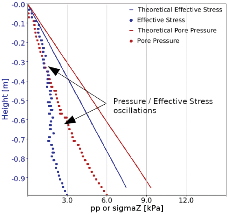
Figure 9: Pressure oscillations that are present during run-time of the system before it has reached equilibrium. Investigations showed that this numerical artifact is due to the presence of the drag term aC∣c in Eq. (17)

3.2 The Cryer Sphere Problem

In this second example, we attempt to validate the performance of our proposed technique by applying it to the standard Cryer sphere problem [44]. This simulation requires tracking the pore pressure in response to a constant increase in the pressure within the sample medium followed by a steady decrease back to zero. This type of behaviour is commonly referred to as the Mandel-Cryer effect [45]. Cryer developed an analytic expression for the pore pressure evolution at the centre of a poroelastic sphere subjected to external pressure. The sphere has no initial stress or pore pressure, and the fluid is allowed to drain freely from its surface. Formal analysis predicts that the pore pressure at the centre begins to increase, reaches the level of the applied pressure and then continues to rise to some peak value. Then, as the fluid is allowed to drain, the pore pressure decreases again. Since this problem is fully dynamic, it is a good test for assessing the accuracy of the component T1 in Eq. (29). Notice, however, that this problem is not purely concentrated on T1 as the drag term aC∣c will still play a role in the evolution of the problem.

An MPM model was constructed to investigate this effect. A two-dimensional half-circle can visualise the inherent symmetry of the whole three-dimensional sphere (see Fig. 10. The grid has dimensions 1×0.5×0.04 metres with cubic cells of side 4 cm that contain eight particles each. The effective stress and pore pressures in the particles are initially zero and the material properties used in the experiment are listed in Table 2. A 10 kPa load was applied to the surface and a drained boundary condition was applied by setting the pore pressure of the surface particles to zero after each time step.

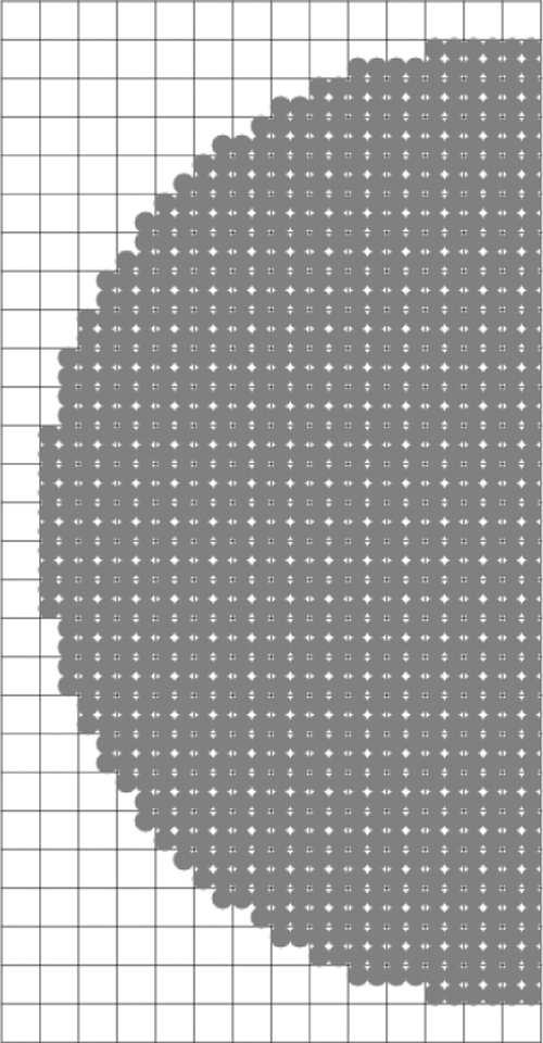
Figure 10: The semicircle used to simulate the Cryer sphere problem. Square cells represent the cells of the background grid and grey points are the particles used to represent the disk

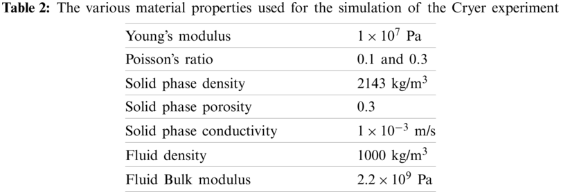
Fig. 11 shows a comparison between our numerical results and the analytical prediction of the pore pressure at the centre of the sphere. We have encouragingly good agreement with the analytic results as well as against previous simulations reported in the literature [24,46]. We notice that at some point, our solution deviates slightly from the analytical expressions. This is especially evident for the case where the Poisson’s ratio was set to 0.1, as shown in the top panel of Fig. 11. Further investigations suggested that this effect can be ascribed to the observation that the regular MPM background grid cannot faithfully capture the perfect boundary of the sphere. A grid made of rectangular cells can only approximate the smooth boundary of the disk; an effect that is inherently clear and which is emphasised in Fig. 10. This effect can be mitigated by making the cell sizes smaller.

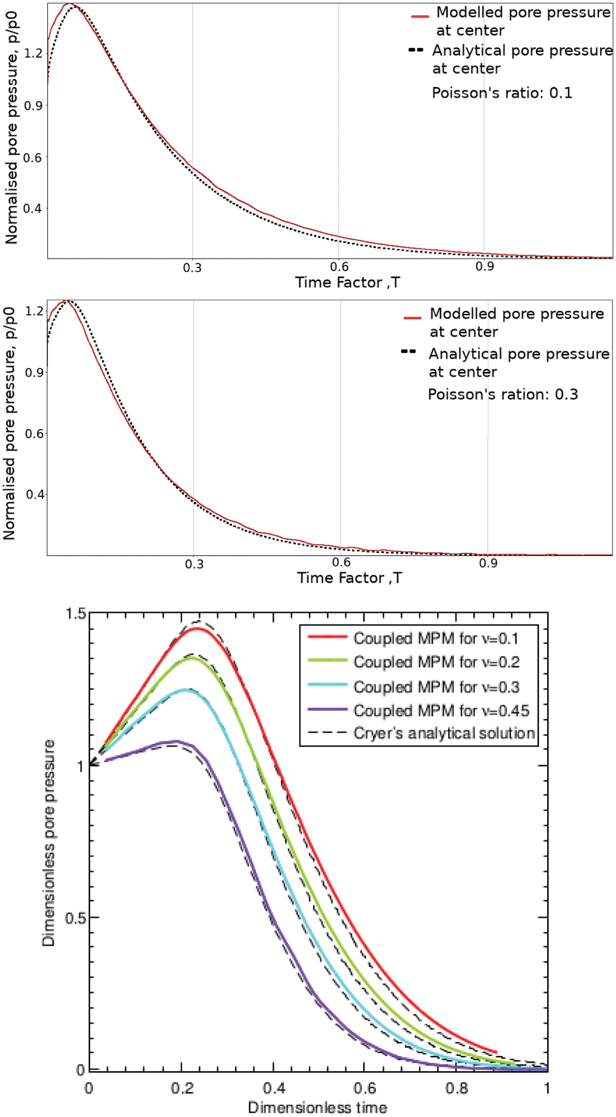
Figure 11: A comparison between the analytical and computed values at the centre of the sphere for Poisson ratio 0.1 (top panel) and 0.3 (middle panel). The bottom panel shows the results of Bandara [24] where ν is the Poisson’s ratio. Our novel MPM provides a good match between the analytical expressions as well as existing MPM formulations

4  A Case Study: The Ernest Henry Mine

Ernest Henry is a copper and gold producing mine situated approximately 40 km North-East of Cloncurry in Queensland, Australia. Initially, the mine design was open pit; however, it introduced underground operations; presently, the deepest part is at about 1.2 km. The mine is seismically active, and its largest recorded event had a moment magnitude of 2.1. Groundwater is a significant problem for engineers working at the mine as they constantly have to drain the deeper levels to prevent flooding. Even though the host rock contains some pore water, it is thought that most of the water is contained in faults that act as the fluid’s principal transport mechanisms. Thus the porosity and conductivity are significantly more than that of the host rock.

On 28 September 2019, the mine drilled an exploration hole in the deepest part of the mine. The hole encountered a geological fault, at which point fluid was ejected from the hole. Several hours later, a large seismic event occurred on the same fault, but several hundreds of metres higher and near development areas. A schematic of the hole and the event location is shown in Fig. 12. This sequence of events raised two particular questions:

•   Was the event triggered by the reduction in pore pressure in the fault?

•   If pore pressure is released in the fault, how does it affect the nearby geology?

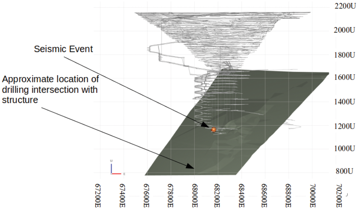
Figure 12: A view looking North of Ernest Henry mine showing where the drilling intersected the fault and the seismic event that occurred several hours later near development areas. Grey lines represent the mine layout at the time of the event and the solid plane represents the fault that is under investigation

The fluid that is trapped within the faults is at high pressure, but this does not imply that it necessarily moves at high speed. The high pressure arises owing to the overburden weight of the fluid, and the porous nature of the rock means that Darcy’s law is applicable. The Institute of Mine Seismology (IMS) was tasked to investigate these questions. An in-house developed version of the standard coupled MPM was used to explore the issues raised. IMS has successfully used their version of the MPM in various three-dimensional numerical studies owing to its ability to simulate large deformation, dynamic problems twinned with the relative ease of building complex mining geometries. It is the prospect of this occurrence at Ernest Henry mine that led to the investigation of a way to simulate the coupled solid-fluid interaction of an heterogeneous medium as it is assumed that the permeability/conductivity of the faults is noticeably different than that of the host rock. We assume that the host rock permeability is very low compared to the rock mass that describes the fault zones and so, to this extent, can be legitimately regarded as a heterogeneous permeability rock experiment. This is a circumstance in which current MPM implementations will likely fail, and we try to overcome this problem using our new method.

A high-resolution single-point coupled MPM model was constructed for the mine. The scheme incorporated an adaptive grid of the type used in the work of [12]; this has the advantage of using various cell sizes with larger ones in areas far from the mine/faults but allowing for finer resolution elsewhere. This refinement facilitates optimal use of computational resources; on the one hand, it dispenses with dense cell packing in regions of little activity while, on the other, it enables high accuracy to be retained near important zones. In our simulation, the largest cells were cubic of side 10 metres while the smallest cubes had an edge of 1.25 metres. The cells that overlapped with the faults were of this smallest dimension, and thus it is remarked that the faults are not thin cracks but instead have a volume consistent with the assumption that they represent intrusions that are infilled by porous rock.

Fig. 13 shows a schematic of the model as well as the material properties. Insitu stresses used in the simulation are listed in Table 3. The model was composed of three materials, one being the host rock while the others were located inside the two faults: the first, identified as fault 6, is the one that intersected with the drill hole, and the second fault, known as the Angry Man Fault, is oriented nearly parallel to fault 6 directly above it. In some places, the two faults are quite close, being within 20 metres of each other, and for numerical purposes, both were ascribed a width of 3 metres and assumed to be porous, so they provided the transport mechanism for the fluid. The total model consisted of approximately 6 million grid cells, with each cell consisting of eight regularly spaced particles.

Figure 13: Left: A view looking north of the mining geometry used in the MPM model. The Angry Man Fault is shown together with Fault 6 which were intersected by the drilling. Right: A zoomed in view of the Angry Man Fault and Fault 6 showing how close they are in space

Several assumptions were made in the model:

•   All materials were assumed to be poroelastic, however, it was assumed that only the two faults were filled with water and that the host rock was dry. This means that fluid flow was confined to be only within the faults.

•   Initial pore pressure in the faults was set to approximately 20 MPa. This is a typical value seen in practice, but precise pressure could not be used as it was not measured by the mine.

•   Draining in the model started approximately 150 metres below the lowest mining level. To reduce the computational complexity, no restriction was placed on the fluid’s outflow rate at the location where the hole intersected the Fault 6.

•   To reduce pressure oscillations caused by the drag term (see Section 3.1) the system was damped such that fd was non-zero in Eq. (21). This ensured that the system remained in a near-equilibrium solution.

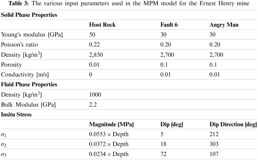
Initially, the model was solved for quasi-static equilibrium by assuming no mining has taken place and using the material properties and stress conditions stated. It was assumed that all materials were dry, which set the rock mass’s undisturbed state. The model was then resolved for the quasi-static equilibrium by removing all particles from the system within the mining excavations. This step represents the current mining state, and it was again assumed that all materials were dry. These two initial steps are common in stress-strain modelling for mining simulations for single-phase problems. Several common stress parameters were selected to quantify the faults as:

•   The major principal stress magnitude σ1,

•   The normal stress to the fault plane σn=σt⋅n, where σt=σn, σ is the element stress tensor and n is the normal direction of the element,

•   The in plane shear stress τ=|σt−σnn|,

•   The excess shear stress, otherwise known as the Coulomb stress [47], defined as σESS=τ−μσn−σc, where μ is the angle of internal friction and σc is the material cohesion. For the purpose of this study we assigned values of 25 degrees and 0 MPa to μ and σc, respectively.

The excess shear stress (ESS) is often used in elastostatic modelling to determine whether a fault may be at risk of slipping within the context of the elastic model. Areas on the fault that display negative (or zero) ESS values are considered stable, whereas areas of positive ESS are liable to slip, or may have already slipped at a prior point. Fig. 14 shows the results of the ESS on both faults at the end of the initial phase. Positive values of ESS are observed on both faults near the location of the seismic event, showing that this area of the fault is at risk of slip even before draining the F6 fault. It is envisioned that since the model predicts that this area is near failure, only minor changes in stress in this area could be sufficient to act as a triggering mechanism for the seismic event. Therefore, for the next phase, we are interested in changes in the selected parameters on the faults, rather than the absolute values as used in Fig. 14.

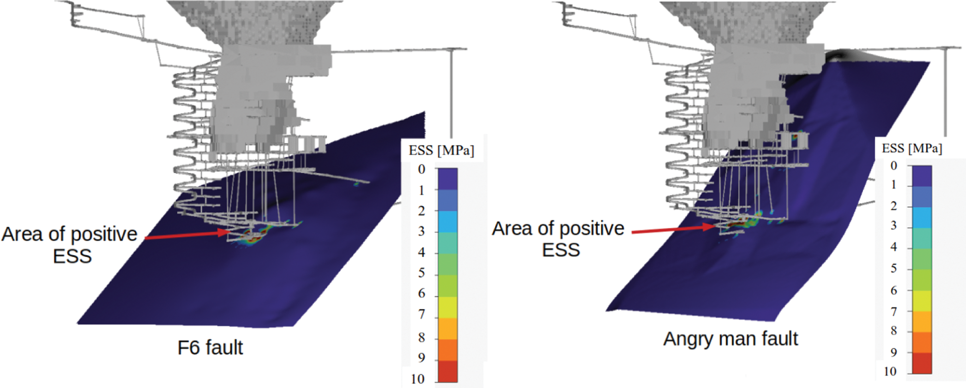
Figure 14: A view looking north of the mining geometry and faults used in the initial phase of the simulation. Left: ESS parameter contoured on the F6 fault. Right: ESS parameter contoured on the Angry man fault. Positive ESS values are visible near development areas where the seismic event occurred. This may be an indicator that this area of the fault was prone to slip, prior to draining the fault

The draining phase was initiated by modifying the particles that characterise the faults. It was assumed that these were fully saturated, and a 20 MPa pore pressure was assigned to each particle. To preserve quasi-static equilibrium, the diagonal terms of the particle stress matrix was reduced by 20 MPa, thus ensuring that the total particle stress remains unaltered and Eq. (19) is unchanged. The draining process was then commenced by identifying several particles close to the drain point location and gradually reducing their pore pressures to zero. These pore pressures then remained at zero throughout the remainder of the experiment. Since the simulation was maintained near quasi-static equilibrium, we applied the less stringent time-stepping scheme as discussed in Section 2.3 enabling the calculation to be completed in a reduced time.

Fig. 15 shows the pore pressure inside the fault at two instances, namely at 5 sec and 41 sec after the commencement of draining. Figs. 16 to 19 summarise the form of four of the key parameters evaluated at the faults. The left panels of each of these figures show the Angry Man’s changes, whereas the right insets show the changes on the F6 fault. The values of the major principal stress σ1 and the normal stress σn increased on the F6 fault, whereas the values of shear stress τ and ESS decreased as the fault drained. This shows that draining has a positive effect on this fault, and it is less likely to slip due to the fault becoming more clamped (opposite ends of the fault plane is being squeezed together). Although less dramatic, the opposite effect is observed for the Angry man fault. The values of σ1 and σn decreased on this fault, whereas τ and ESS increased. This shows that draining of the F6 fault unclamps the Angry man fault and can potentially make the fault more hazardous.

Figure 15: Left: Pore pressure in the F6 fault after 5 sec of draining. Right: the pore pressure after 41 sec of draining. The arrow indicates the location at which the fluid was drained

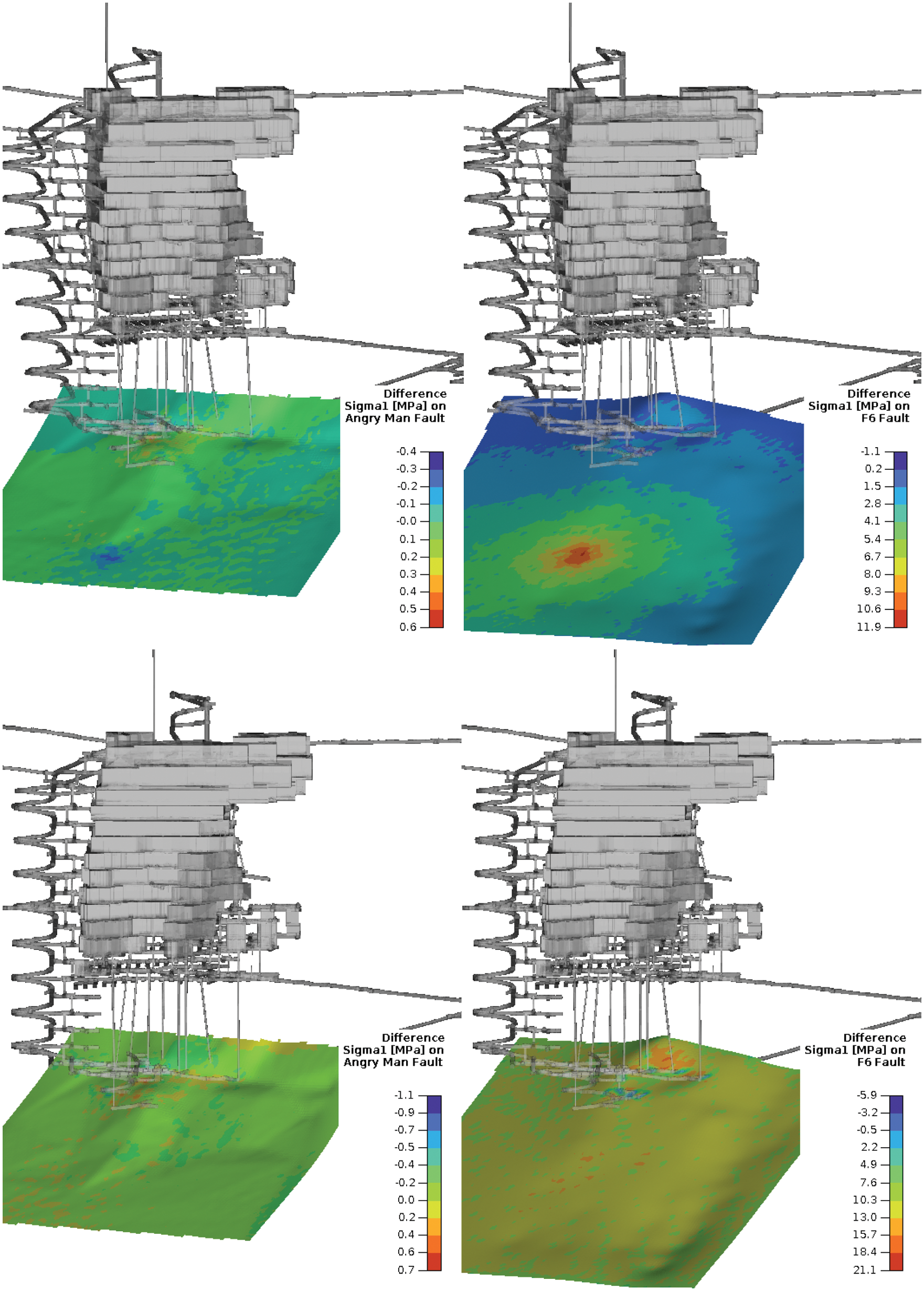
Figure 16: Top row: change in σ1 after 5 sec draining on both faults. Bottom row: change in σ1 after 40 sec draining on both faults. Left column: the Angry Man fault. Right column: the F6 fault. There are minor changes in σ1 on the Angry man fault whereas the principal stress near the drain point on the F6 fault are more significant

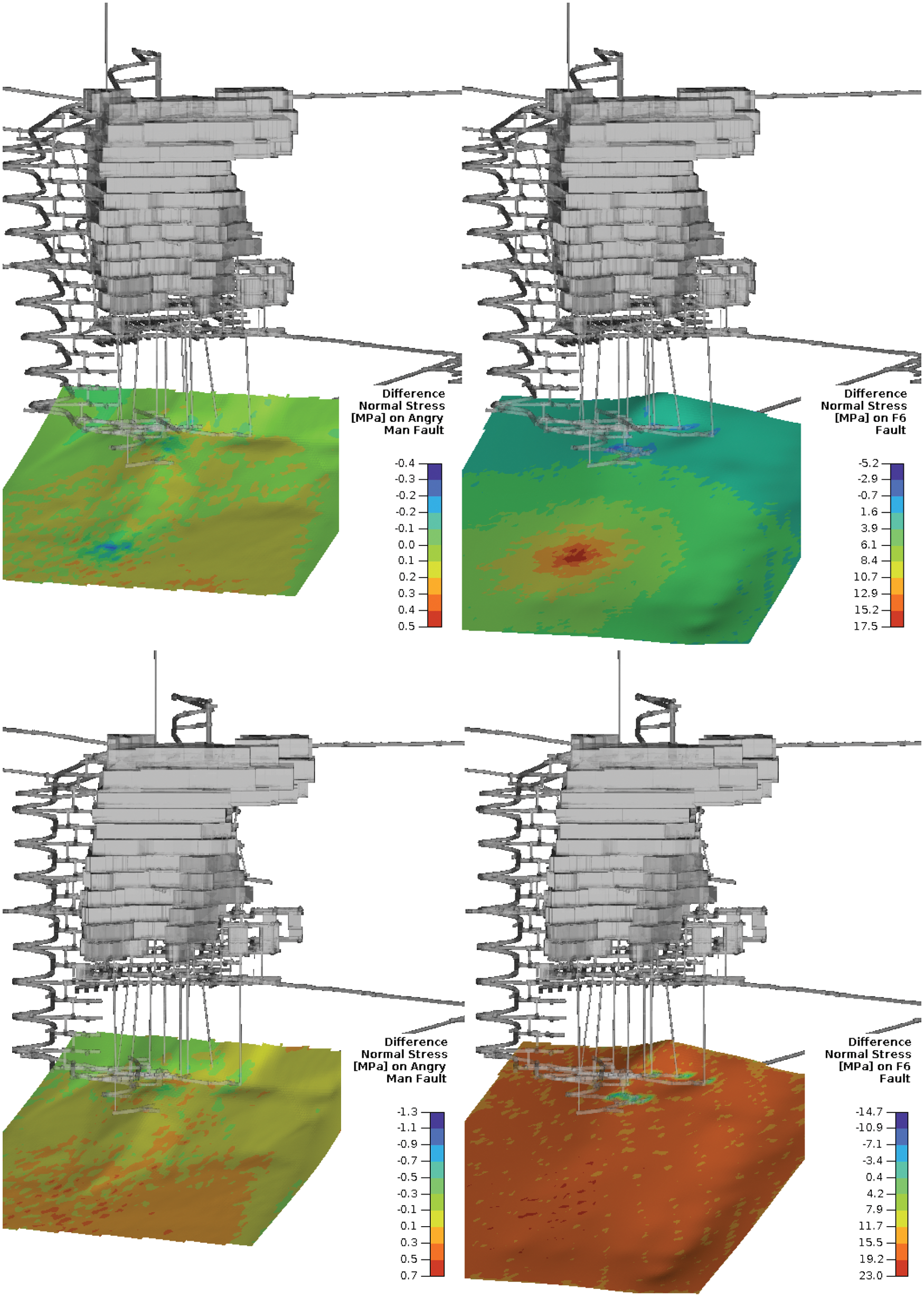
Figure 17: Top row: change in σn after 5 sec draining on both faults. Bottom row: change in σn after 40 sec draining on both faults. Left column: the Angry Man fault. Right column: the F6 fault. There are minor changes in σn on the Angry man fault and and a large increase in σn on the F6 fault. This indicates that the F6 fault be being more clamped whereas the Angry Man fault is being unclamped

Figure 18: Top row: change in τ after 5 sec draining on both faults. Bottom row: change in τ after 40 sec draining on both faults. Left column: the Angry Man fault. Right column: the F6 fault. There are minor changes in the shear stress for both faults

Figure 19: Top row: change in ESS after 5 sec draining on both faults. Bottom row: change in ESS after 40 sec draining on both faults. Left column: the Angry Man fault. Right column: the F6 fault. ESS decreased significantly on the F6 Fault, indicating the fault is less likely to slip. The ESS on the Angry man fault increased slightly near the drain area, and more significantly near development areas. This could potentially be a trigger for the seismic event

The results as outlined in Figs. 16 to 19 illustrate the importance of taking pore water into account in numerical simulations for mines such as Ernest Henry. Simulations that do not allow for this may show that both faults are stable and unlikely to fail. We have shown this in Fig. 14. Our models suggest that pore water is indeed essential in assessing the stability of the two faults. Even though pore pressure reduction in the F6 improved its stability, one may imagine that the opposite could occur; if pore pressure were to increase, then the fault becomes less stable. Furthermore, the effect of reduction in pore pressure may affect surrounding geological structures. In this case, the Angry Man fault conditions worsened, and even though the result was less pronounced than for the F6 fault, one may speculate that the reduction of pore pressure of the F6 fault could indeed be a triggering mechanism for the seismic event.

Video clips of the simulations of each modelling parameters used in this experiment can be obtained from:

•   http://downloads.imseismology.org/numericalmodelling/mpm/ess.m4v Link to video clip showing Excess Shear Stress changes as the F6 drains

•   http://downloads.imseismology.org/numericalmodelling/mpm/shear-stress.m4v Link to video clip showing τ changes as the F6 drains

•   http://downloads.imseismology.org/numericalmodelling/mpm/sigma1.m4v Link to video clip showing σ1 changes as the F6 drains

•   http://downloads.imseismology.org/numericalmodelling/mpm/normal-stress.m4v Link to video clip showing σn changes as the F6 drains

In each of the clips we show how the draining of the F6 fault changes the properties of both itself and the nearby Angry man fault. These clips are free to download and redistribute.

5  Concluding remarks

A fully coupled two-phase three-dimensional MPM has been developed to model stress changes caused by fluid-filled rock in mining. This has been accomplished by modifying existing coupled MPM approaches to incorporate the description of mediums with heterogeneous permeability. Two verification examples were used to test the accuracy of the numerical model, and good agreement was observed in both cases. These benchmarks provide confidence that our methodology has value when modelling real mining cases in which a seismic event is likely triggered due to pore pressures changes caused by draining of a nearby fault. In this experiment, we have shown that even though the effective stress changes on the fault were relatively small, it was nonetheless still sufficient to play a role as a provocative mechanism for the event.

The case study at Ernest Henry mine highlights the importance of accounting for the effect of pore water in mining simulations, an effect that is often neglected. However, as mining methods become increasingly complicated, so the need for more advanced multi-phase numerical simulations grows. This is especially true for simulations of mine tailings dams for which the presence of fluid can play a central role in determining the outcome of experiments.

Our method can benefit from further improvement in two areas; a more advanced soil model might be implemented for dealing with problems involving partial saturation, and the numerical fluctuations in pore pressure could be reduced when dealing with dynamic problems. Further research in both these aspects must be pursued.

An intriguing avenue for future work would be an investigation of the relationship between our formulation and the innovative technique known as peridynamics. This is a novel non-local method that has been suggested as a vehicle for simulating hydraulic fractures [48,49]. It would be of interest to see how our method might be adapted to hydraulic fracturing scenarios as this is typically a multi-phase problem. This can not be done immediately since our current technique assumes that the faults are of finite thickness intruded by a porous material as opposed to being thin cracks. Further work is required to see if our method can be extended to address this important issue.

In summary then, our new model appears to show promise for modelling multi-phase coupling mechanisms in realistic mining situations. What we have described here is a first step in this direction, and extensions to further real case studies is the obvious way forward. As the catalogue of simulations increases, this would enable us to predict those circumstances in which mine sites might benefit from our ideas. One particular attraction of our suggestions is the fact that they can be incorporated into conventional MPM methods with only marginal extra computational cost.

Acknowledgement: We would like to thank Ernest Henry mine for allowing the use of their data in our case study. We are grateful to the reviewers for numerous suggestions and additional references that have significantly improved the quality of the manuscript.

Funding Statement: The authors received no specific funding for this study.

Conflicts of Interest: The authors declare that they have no conflicts of interest to report regarding the present study.

This work is licensed under a Creative Commons Attribution 4.0 International License, which permits unrestricted use, distribution, and reproduction in any medium, provided the original work is properly cited.