Computer Modeling in Engineering & Sciences

DOI: 10.32604/cmes.2022.016705

ARTICLE

Fast and Accurate Thoracic SPECT Image Reconstruction

Afef Houimli1,*, IssamBen Mhamed2, Bechir Letaief1,3,4 and Dorra Ben-Sellem1,3,4

1University of Tunis El Manar, Higher Institute of Medical Technologies of Tunis, Research Laboratory in Biophysics and Medical Technologies LR13ES07, Tunis, 1006, Tunisia
2University of Tunis, Higher National School of Engineers of Tunis, Signal Image and Energy Management Laboratory: LR13 ES03 SIME, ENSIT, Montfleury, 1008, Tunisia
3Faculty of Medicine of Tunis, University of Tunis El Manar, Tunis, 1007, Tunisia
4Nuclear Medicine Department, Salah AZAIEZ Institute, Tunis, 1006, Tunisia
*Corresponding Author: Afef Houimli. Email: houimliafef13@gmail.com
Received: 18 March 2021; Accepted: 17 June 2021

1  Introduction

Single-Photon Emission Computed Tomography (SPECT) is an emission imaging modality based on the administration of radiopharmaceuticals to patients. A gamma photon detector rotates around the patient to register multiple projections of the radioactive concentration at different angles. A computer must reconstruct these projections to obtain a 3D volume of the object. Tomographic reconstruction aims to extract axial, coronal and sagittal slices of the object from its finite number of projections. This reconstruction reflects the functional information about metabolic activity and lets the doctors effectively diagnose the radiopharmaceutical distribution in anybody slice [1]. Historically, reconstruction is carried out slice by slice, all the reconstruction algorithms have reduced the 3D-image reconstruction to a 2D-image reconstruction by converting a 2D-projection plan into a 1D-sinogram (profile) to generate axial slice images of the object. These algorithms are called 2D-reconstruction algorithms [2]. Recently, due to the growth in the speed of the processor’s modern computer and the availability of the capacity memory chips, a 3D-image reconstruction algorithm has appeared. These algorithms enable the simultaneous and complete reconstruction of projection data. The 3D-image reconstruction algorithms convert the input sequence of image projection to a 3D matrix, then allow a simultaneously 3D axial slice image reconstruction and not successively in the interactive calculation which is the case of 2D-reconstruction. These algorithms need a large matrix to consider photons detected in the out of projection plan [3]. Two classes of reconstruction algorithms are developed: analytic reconstruction and iterative reconstruction. Therefore, due to the radioactivity disintegration, to the acquisition and the reconstruction algorithms procedure, the reconstructed SPECT image suffers from poor spatial resolution, bad contrast and an important noise level which makes it difficult to detect the bone lesions and allows an inaccurate diagnosis. The analytic reconstruction, such as Filtered Back-Projection (FBP) [4], generated significant artifacts and induced more noise because of the limited number of acquiring projections [5]. On the other side, the iterative method improves the reconstructed image quality and decreases the produced artifacts [6]. Maximum Likelihood Expectation Maximization (MLEM) is the most common iterative algorithm, which was proposed by Bruyant [2] and afterward enhanced in acceleration using the Ordered Subset Expectation Maximization (OSEM) algorithm [7–9]. However, the quality of the produced image with the last technique becomes noisier by increasing the number of iterations and subsets [1,10]. Poisson noise is highly dependent on the signal. Therefore, it is difficult to separate the signal from the noise [11]. Then, to improve the quality of the reconstructed images, several studies based on the standard reconstruction methods have been published. Single scale filtering, such as Stationary Filtering operations, either linear or nonlinear, are commonly used. Because of its limited consideration of count distributions and noise level, these filters decrease noise variance but degrade image contrast and detail [12]. Adaptive and nonstationary filters have also improved the reconstructed SPECT image quality [13–16]. These filters are characterized by the selection criteria used for smoothing regularization. Besides, this approach provides filtered image textures, different from those of the original image. In [17], a comparison has been made between FBP, OSEM with adaptive filter (Metz) and OSEM with non-adaptive filter (Butterworth). Different combinations have been applied to bone SPECT images of the spine with and without scatter correction. This work showed that the OSEM reconstruction combined with Metz filter or Butterworth filter gives a good result in homogenous regions. Still, it blurred the edges and degraded the image resolution. To overcome these limitations, multi-scale denoising approaches have been suggested for image denoising in SPECT reconstruction. Contrary to the single-scale filtering approach, multi-scale methods separate the signal of interest from the noise components and analyze each component into different sub-band coefficients with the adaptive denoising algorithm. Especially, Wavelet transform [18–22] has been proposed. In their work, Wen et al. [18] showed that the SPECT reconstruction algorithm based on Wavelets transform reduces the noise in the reconstructed SPECT image. However, because of the signal-dependent Poisson noise in the acquired projection, this approach does not provide a good representation of the anisotropic elements in the reconstructed SPECT images. Other families of multi-scale approaches were proposed for the reconstructed SPECT image denoising, such as the Curvelet multi-scale method [23]. The Curvelet transform is based on the anisotropic graduation principle, which is quite different from isotropic wavelet scaling. These characteristics are beneficial for the development of denoising SPECT image algorithms. Low density characterizes very high signals that have line, curve and hyperlink singularities [24].

On another side, the cascaded hybrid framework has been proposed for improving the quality of SPECT image reconstruction. In their work, Tiwari et al. [25] proposed a model composed of two iterative algorithms and an edge-preserving function in the iterative denoising step, which is the anisotropic diffusion (AD). This study shows that the proposed model can deblur the reconstructed image SPECT in lower computational time. Recently, Machine learning (ML) has been implemented for various medical imaging modalities such as Magnetic Resonance Imaging [26], Computed Tomography [27], Positron Emission Tomography [28] and SPECT [29–31]. Several studies proved the efficiency of this technique to produce high image quality with a substantial reduction of noise and blurring artifacts. However, one of the principal drawbacks of these methods is that the resulting neural network is not a feed-forward formulation. Hence, their utilization can be more likely in applications where high precision exceeds the reconstruction time [32]. In this work and based on the prior results, we propose a new algorithm for improving the reconstructed bone SPECT image quality. The proposed method is based on a new combination of multi-scale denoising, fast 3D-OSEM reconstruction algorithm and one of the newest anisotropic diffusion models. Two simulated phantoms and preclinical bone exam data were used to evaluate the performance of the proposed approach. A comparative study is performed between the proposed algorithm and four states of the art techniques for SPECT image reconstruction: MLEM, 2D-OSEM, 2D-OSEM + Metz filter and CNNR algorithms.

This paper is organized as follows:Section 2 discusses the proposed method. The obtained results are presented and analyzed in Section 3. Section 4 illustrates the conclusion and future directions.

2  Materials and Methods

2.1 Reconstruction Algorithms

Tomographic reconstruction aims to estimate an explored region from a finite number of acquired projections. The reconstruction algorithms present the region to be explored in multidirectional slice images. This reconstruction reflects functional information of metabolic activity in any slice of this region. There are two types of reconstruction, analytic and iterative.

2.1.1 Analytic Reconstruction

Two classes of the analytic algorithm are developed, simple back-projection (SBP) and filtered back-projection (FBP) [4]. FBP reconstruction combines two steps: filtering the data and back-projection of the filtered data using the direct inversion of the radon transform. FBP is the most widely used because of its simplicity and speed. However, due to thelimited amount of projection data, it can generate significant artifacts and induce more noise [5].

2.1.2 Iterative Reconstruction

The iterative algorithm consists of linking numerous forwarding projections and back-projection operations since initial data. The initial image is an estimated image created arbitrarily. The successive estimate stopped when the projection of the reconstructed image similar to the measured projections. These methods reduce the significant artifacts and enhance the reconstructed image quality.

•   The principle of some iterative algorithms (ML-EM OS-EM)

The (ML-EM) algorithm is the standard iterative reconstruction method which consists of two alternating steps: an E-step creates a function for computing the expectation of the log-likelihood which evaluates the similarity between simulated and measured sinograms, and an M-step which finds the next estimate image by maximizing the expected log-likelihood found on E-step while taking into account the fact that the first estimate image is positive and that a noisy Poisson attains the measured sinograms. The MLEM algorithm is presented in Fig. 1.

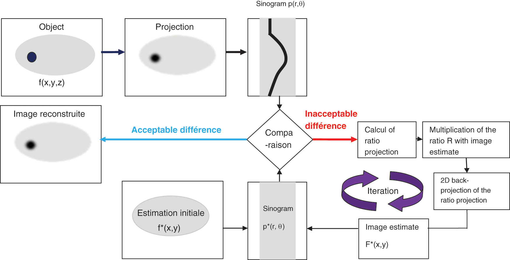
Figure 1: MLEM algorithm

The OSEM algorithm [6–8] is composed of ordered subsets ported to the MLEM algorithm which allows a much faster convergence, compared to the original convex algorithm, and an easy parallelization. The principle of this algorithm is based on the division of the acquired projections into ordered subsets for the calculation of iteration. Subsequently, the MLEM algorithm is applied to each subset in turn. The update of the estimated images with the OSEM method is done with the corresponding subset. The operation is repeated until the last chosen subset.

The iterative reconstruction algorithms improve the reconstructed image quality and reduce the generated streaking artifacts [5]. However, these algorithms still suffer from the slowness of convergence and the quality of the produced image which becomes noisier with the increase in iterations and subsets.

2.2 Proposed Method

In this section, we present the proposed algorithm to improve the quality of reconstructed bone SPECT images. We start with a global introduction of the proposed model. Then, we detail each step. Fig. 2 presents an overview of our method, which is clearly illustrated in Fig. 3. In our work, we used three SPECT databases. Each database is composed of a SPECT image. This image is a sequence of 128 projections. These projections were acquired according to 128 projection angles. Each input projection is a 128 * 128 size matrix. After the projection sequence of the denoising step, a sequence of filtered sinograms was assembled then reconstructed with a Fast 3D-OSEM reconstruction. An optimization step was carried out to obtain the best quality of axial slices. Finally, we extract a sequence of coronal slices and a sequence of sagittal slices from the sequence of the improved axial slices.

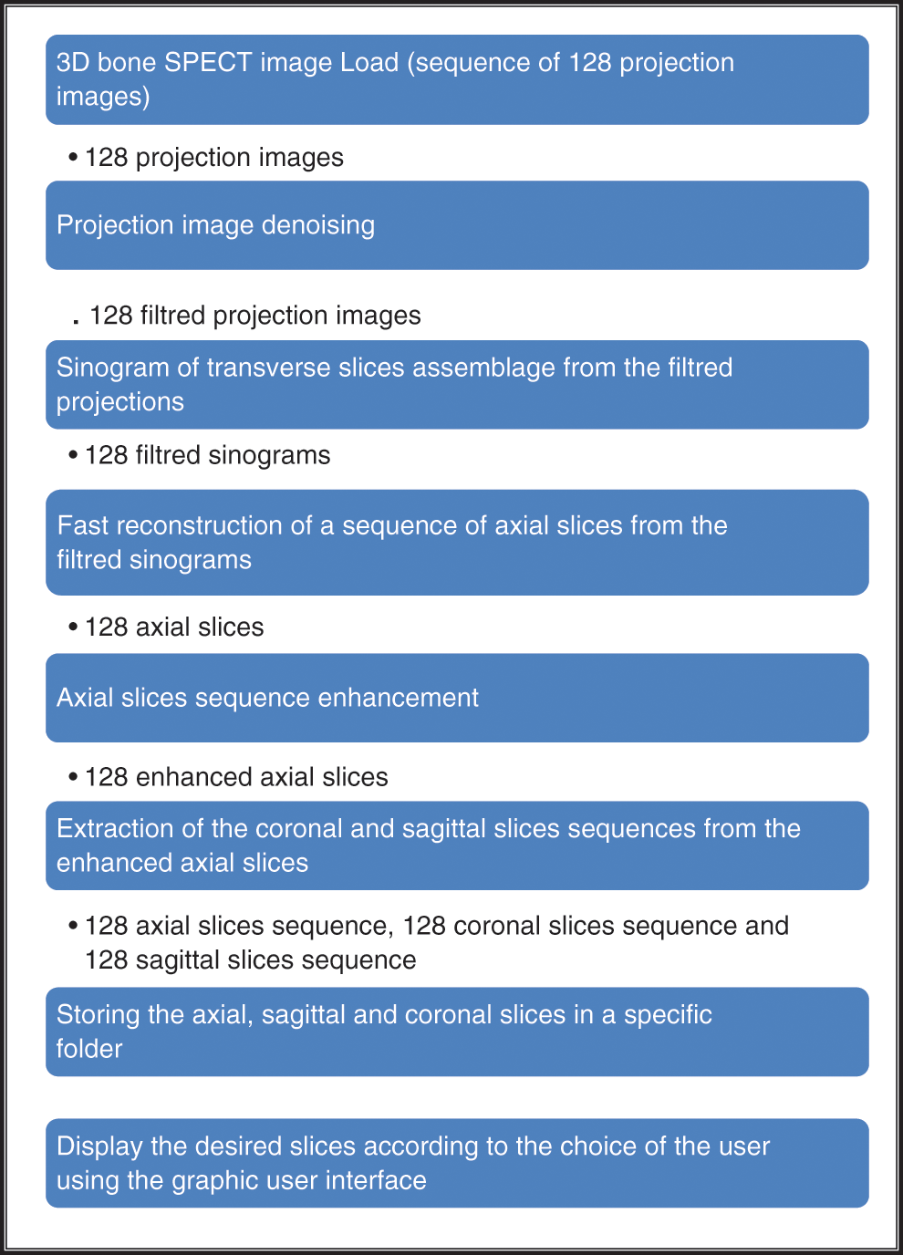
Figure 2: Diagram of the main work for 3D bone SPECT image reconstruction

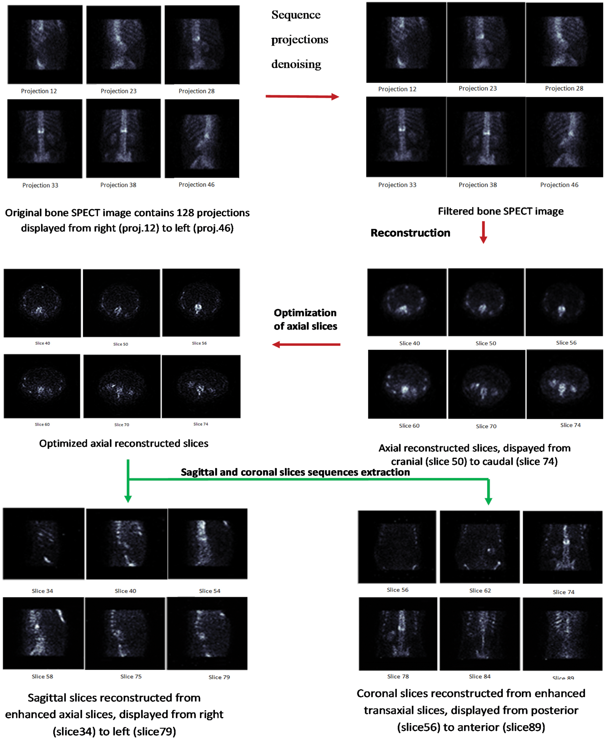
Figure 3: Proposed method

In the following, we will introduce our methodology in subtleties by concentrating on the next steps.

2.2.1 Projection Denoising

To reduce the noise efficiently in the projection image as much as possible with preserving the image details, we explore the benefits from the complementary properties of both the Wavelet transform and Curvelet transform. During the first step, we exploited the ability of Wavelet transform to detect the edges. Indeed, we applied the Curvelet transform on the residual image. The later image is the result of subtracting the original image from the filtered image. The filtered image is composed of fine details, structure and noise.

Wavelet transforms (DWT)

The DWT is a powerful multi-scale transform for denoising because of its ability to separate noise from signal [1,33]. It decomposes the SPECT origin projections by filter banks into a set of frequency band images. This transform uses low pass filters and high pass filters to extract the significant wavelet coefficients called approximation and remove the non-significant wavelet coefficients called details. In this work, we used the Daubechies Wavelet transform with 5 scales because, by set learning, we found that this algorithm provides the best performance of bone SPECT denoising.

Curvelet transforms (CWT)

To analyze the anisotropic features of projections, we used the second generation of Curvelet transform (Candes, 2006) [34], which is considered as one of the most important directional representation systems [35]. It is a multi-scale and multidirectional transform with frame elements indexed by the scale, location and directional parameters, with the frame’s shape localized in the spatial and frequency domains. It showed higher levels of directionality and anisotropy. As the construction of this transform is done in the Fourier domain; the generating Curvelet ωj,0,0 at scale 2−j is defined via:

W^j,0,0(reiθ)=2−3j4.A(2−jr).B(2j2+1πθ) (1)

where α=reiθ are the polar coordinates. A and B are respectively the radial window and the angular window. They have to satisfy proper admissibility conditions.

At scale 2–j, the Curvelet’s family {W^j,k,l}j,k,l is constructed by translation and rotation of the generating Curvelet Wj,0,0, their expression is defined via:

Wj,k,l(x)=Wj,0,0(Rθj,k(x−Slj,k),for xϵR2 (2)

where Rθj,k presents the rotation matrix:

Rθj,k=(cos⁡θj,ksin⁡θj,k−sin⁡θj,kcos⁡θj,k)

θj,k denote the scale-dependent rotation angles and Slj,k denote the scale-dependent locations which are expressed by:

θj,k=k.π2−(j/2)−1,−2(j2)+1≤l≤2(j2)+1; (3)

Slj,k=Rθj,k−1(l12j,l22j/2),l=(l1,l2)ϵZ2 (4)

The refraction coefficient of each unknown function f is expanded in term of curvelet via:

f=∑⟨Wj,k,l,f⟩Wj,k,l (5)

where j is the scale parameter, l is the location parameter and k is the location parameter that corresponds to directional features of f.

Combined denoising step

As explained previously, WT and CT present complementary behaviors; the number of directional elements in the wavelets is fixed independently from the scale. Therefore, the WT does not perfectly restore the anisotropic element like the outlines and the edges. While the CT presents high directional anisotropy elements, this transform does not handle small isotropic elements properly. So, we exploited both transforms in the same model to improve the denoising methodology of acquired projections.

The combined denoising scheme is illustrated in Fig. 4. We applied the Curvelet transform on the residual image. The residual image is the result of subtracting the filtered image from the original image. This residual image contains structures, noise and details. This is clearly illustrated in Fig. 5. By applying the CT denoising to the residual image, we detect the structures and features lost during the WT’s denoising in the first step. The filtered residual image by the CT will be fused with the initial noisy image processed by WT.

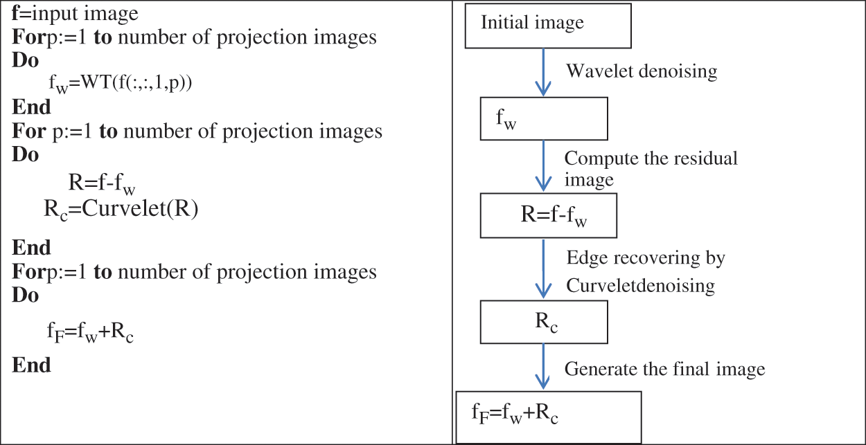
Figure 4: Projection images denoising

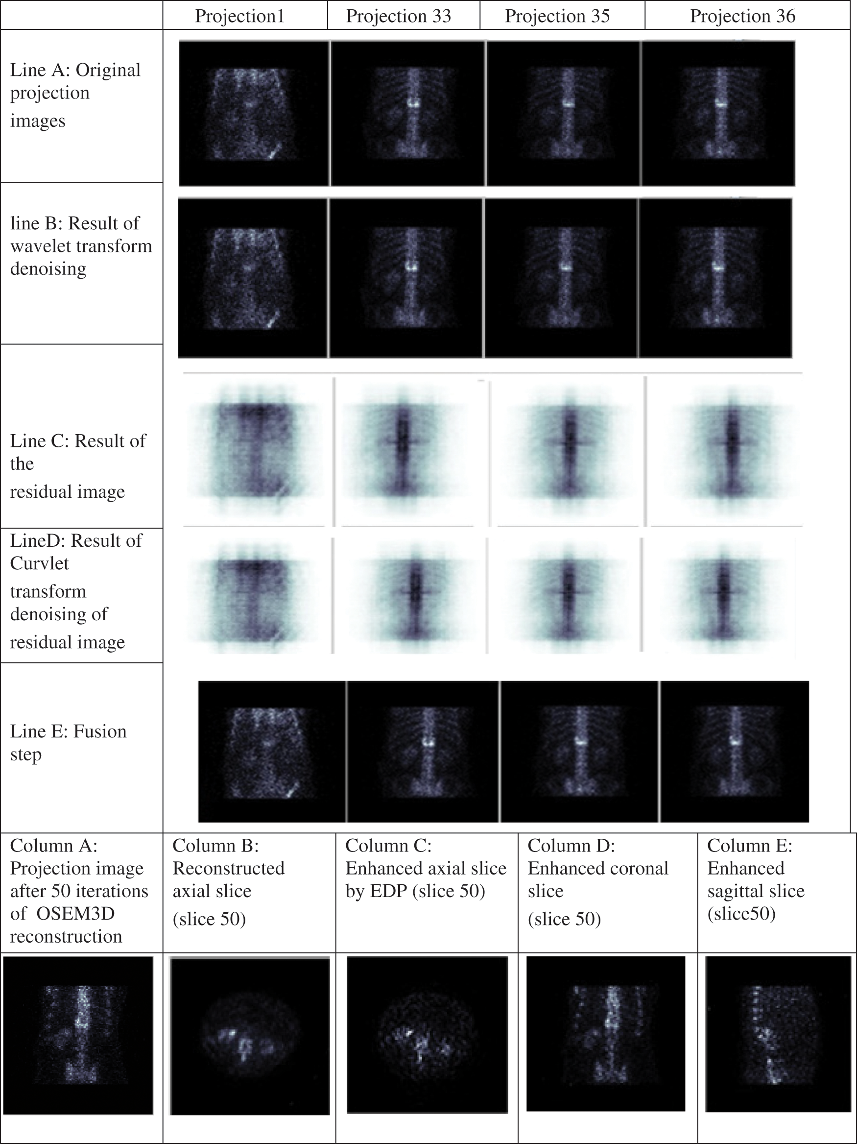
Figure 5: Different results of the proposed algorithm at bone level images

2.2.2 Fast 3D-OSEM Reconstruction

To reduce the image reconstruction time, we used the 3D-OSEM reconstruction algorithm which allows a simultaneous reconstruction of all axial slices. In the first step, the sequence of projection data is converted into a 3D matrix. Therefore, a 3D-sinogram is assembled simultaneously from the projection image matrix. Then and in the second step, a 3D image of axial slices is reconstructed simultaneously from the 3D matrix of sinograms and not successively which is the case of 2D OSEM reconstruction (slice-by-slice) [36,37]. For N iterations and M subsets, the 3D-OSEM resulted image is computed using the following equation [38]:

fks+1(St)=fks1∑kϵStpkj3−D∑kϵStpkj3−DCk∑k=1Kpkjfks (6)

where: fks and fks+1 are the estimated images at voxel j and sub-iteration s and s + 1, respectively, with 1<k<K, K is the total number of voxels along ray j.

Ck: is the measured projection at projection bin k.

pkj is the transfer matrix which presents the probability that a photon emitted from the voxel image j is detected in projection bin k.

2.2.3 Optimized Axial Slice Sequence Enhancement

Slices reconstructed with the 3D-OSEM technique are still noisy with attenuated details which agree with the researchers’ results [9,10]. Therefore, the image must be processed to enhance and sharpen different details of the slice image. We applied a new modified anisotropic diffusion model called Partial Differential Equation (PDE) on the reconstructed slices to perform this operation. This model has been used as an adaptive edge-preserving smoothing technique for edge detection [39], denoising, enhancement [40] and segmentation [41–43] of image. This is a nonlinear (PDE) based on a diffusion process. This model is a modification of Perona and Malik’s (1990) equation and is expressed as follows:

∂fj(m,n)(Sm)(x,y)∂t=div[ct(x,y).∇fj(m,n)(Sm)(x,y)] (7)

where fj(m,n)(Sm)(x,y) is the gray level at coordinates (x, y) of the image at iteration step t, div is the divergence operator, ∇fj(m,n)(Sm)(x,y) is the local image gradient and ct(x,y) is the diffusion coefficient introduced which aims to remove noise without blurring or dislocating the useful edge information of the images.

The PDE is an anisotropic diffusion model [44]. It is based on a developed stop edge function. This diffusion method allows smoothing the background and sharpening intra-region even in low contrast regions contrary to the Perona-Malik model [45], which returns small values in regions with significant variations in intensity and large values in regions few or no intensity fluctuations. This developed diffusion model is based on modifying the classical diffusion rule using a nonlinear sigmoidal function to generate various degrees of edge sharpness.

In this model, a median filter is applied to the gradient of the image. The PDE algorithm is given as follows:

∇∗fj(m,n)(x,y)=median(∇fj(m,n)(x,y) (8)

Compute the gradient and the diffusion function.

Compute the sharpening diffusion coefficient.

υ(∇fj(m,n)(x,y))]=α[1−g(∇fj(m,n)(x,y))] (9)

Then a refining function is added to the edge-stopping rule. The proposed formula is given by Eq. (10)

g(∇∗fj(m,n)(x,y))=1[1+(∇∗fj(m,n)(x,y)K)2][−11+exp⁡(−p*(∇∗fj(m,n)(x,y)K)] (10)

where

1[1+(∇∗fj(m,n)(x,y)K)2] is the edge stopping rule proposed by Perona and Malik

11+exp⁡(−p*(∇∗fj(m,n)(x,y)K) is the refining function

where K is the thresholding and α is the weight of the sharpening coefficient function.

2.3 Coronal and Sagittal Slice Extraction

We extracted a sequence of coronal slices and a sequence of sagittal slices from enhanced axial slices. Each slice has a thickness equal to 1 pixel, displayed respectively from posterior to anterior and right to left, allowing the doctors to perform a diagnostic in any slice of the object.

To choose the best combination of parameters for the proposed algorithm, we applied our algorithm on 31 abnormal bone SPECT images, and each image contains hyperfixation in the bone. Then, we calculatedthe means contrast, the means contrast to noise ratio (CNR) and the means signal to noise ratio (SNR) of the resulted slices as described in the following equations:

Contrast=|µs−µbµb| (11)

CNR=|µs−µbσ| (12)

SNR=µs−µbµbb (13)

where µs is the maximum count in normal bone, µb is the maximum count in hyperfunctionning bone, µbb is the minimum count in background and σ is the standard deviation in background.

We performed the Jarque-Bera test to test whether the series were usually distributed. From the statistics, Jarque-Bera normality, the assumption can accept some values during our study. Performing the One-Way ANOVA-test, the optimum combination of parameters for the proposed method has the highest value of contrast, CNR and SNR. Numerical results of all patient data revealed that maximum contrast, CNR and SNR could be obtained using the Curvelet transform with a threshold value equal to 0.01, the Wavelet transform with an order equal to 4, a PDE model with K = 0.2 and α = 0.01, combined with an OSEM3D algorithm with 4 subsets and 8 iterations.

3  Results and Discussion

This section presents a description of phantoms and bone SPECT database obtained from the nuclear medicine department of the National Oncology Institute “Salah AZAIZE” of TUNIS. Then, we present the different results and performance analyses of the proposed method.

3.1 Database Description

The proposed method was tested on two different SPECT phantoms: Shepp-Logan phantom and Jaszczak phantom, and our bone SPECT database.

3D-Shepp–Logan phantom

To evaluate the robustness of our reconstruction algorithm, we used a tomographic digital Shepp–Logan phantom. The distribution of projection data is assumed to be generated by 128 angular views (distributed in the range of 180 degrees). Fig. 6 presents the Shepp-Logan phantom image at projection 64.

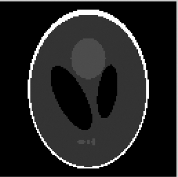
Figure 6: Shepp-Logan phantom (Projection 64)

Four objective criteria were used to evaluate the performance of the reconstructed axial slices. They are the Mean Square Error (MSE) [23], Mean Absolute Error (MAE), Structural Similarity Index (SSIM) [46], the Pearson Correlation Coefficient (PCC) [47] and execution time.

3D Jaszczak phantom

To evaluate the accuracy of our reconstruction algorithm, we used a Data Spectrum Corporation Jaszczak phantom composed of bars and six cold spheres of diameter: 31.8, 25.4, 19.1, 15.9, 12.7, 9.5 mm. The Jaszczak phantom was filled with a radioactive solution containing 2 mCi of a uniform 99mTc solution. The acquisition of the Jaszczak phantom image was affected using 180° non-circular orbit for each detector, with 96 projection angles, a 128 * 128 matrix size, and an electronic zoom of 1/1 provided a pixel size of 4.795 mm. Fig. 7 presents the Jaszczak phantom image at projection 76.

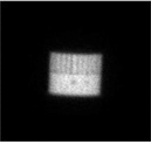
Figure 7: Jaszczak phantom (Projection 76)

The tomographic Jaszczak phantom image reconstruction using the proposed method was performed using 8 iterations and 4 subsets, combined with a Curvelet denoising wavelet with a threshold value equal to 0.01 and an EDP thresholding value K = 3 and weight of sharpening coefficient function α = 0.5.

To evaluate the reconstructed image quality, we draw a circular region of interest (ROI)s of 20 cm diameter for each of the 5 jaszczak spheres in the uniform section of the phantom. A background ROI was also created using five (ROI)s on five central slices.

Contrast is calculated using Eq. (11) and CNR is calculated using Eq. (12).

where µs is the mean activity in a single ROI of a cold sphere, µb is the mean activity in a single ROI of background and σ is the standard deviation value in a background region.

Patient exams

A bone SPECT dataset is taken from the nuclear medicine department of the National Oncology Institute “Salah AZAIZE” of TUNIS, which contains 31 bone SPECT exams, 10 males and 21 females aged between 45 and 75. The acquisitions were made using a Symbia gamma camera equipped with a parallel collimatorusing 180° non-circular orbit for each detector with 128 projection angles, a 128 * 128 matrix size, a pixel size of 4.795 mm. For each methodand for 31 bone SPECT exams, we calculated the values of contrast defined in Eq. (11), of the SNR defined in Eq. (13) and of execution time.

3.2 Shepp-Logan/ Jaszczak Phantom Results

The sequence of Shepp-Logan projections was additionally randomized with a Medium Poisson noise level. The Poisson noise level was used by scaling the sinogram value to 50%. Then, we applied the reconstruction methods to the noisy sequence. To present the phases introduced in Section 2.1, Fig. 8 outlines the different results of the suggested method at a gray level Shepp-Logan phantom image at frame 64. Various parameters were tried to get the highest performance.

Fig. 8 shows the robustness and the accuracy of the proposed algorithm in tomographic reconstruction.

Fig. 9 shows the accuracy of the proposed method during the reconstruction technique.

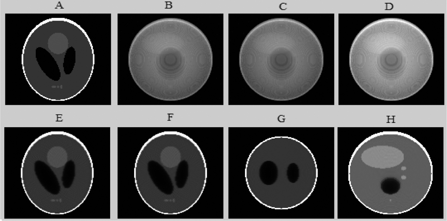
Figure 8: The different results of the proposed algorithm from the tomographic Shepp-Logan Phantom (SLP) image at frame 64. (A) Original (SLP) projection; (B) Noisy (SLP) projection; (C) Projection (SLP) denoised by the Wavelet; (D) Fusion step for (SLP) projection denoising; (E) Reconstructed (SLP) slice; (F) Enhanced axial (SLP) slice by EDP; (G) Coronal enhanced (SLP) slice and (H) Sagittal enhanced (SLP) slice

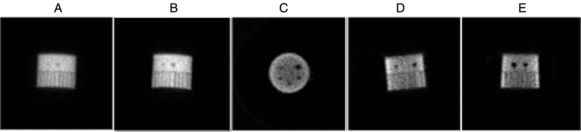
Figure 9: The different results of the proposed algorithm from the tomographic Jaszczak Phantom image (JP) at frame 73, (A) Original (JP) projection; (B) Fusion step for (JP) projection denoising; (C) Reconstructed axial (JP) slice; (D) Reconstructed coronal (JP) slice and (E) Reconstructed sagittal (JP) slice

3.3 Preclinical Data Results

To present the phases presented in Section 2.1, Fig. 5 illustrates the different results of the proposed algorithm at bone level images. Line (A) presents the noisy projection images, Line (B) depicts the results of the projection image denoised by the Wavelet transform, Line (C) illustrates the results of the residual images, Line (D) illustrates the results of the residual image denoised by the Curvelet transform, Column (A) presents the reconstructed axial slice, Column (B) the enhanced axial slice by EDP, Column (C) the coronal enhanced slice and Column (D) the sagittal enhanced slice.

3.4 Performance Evaluation

To evaluate the performance of the proposed method of reconstruction, we conducted a qualitative and quantitative comparison with four other reconstruction approaches available in the literature which are: MLEM [5], OSEM [6], 2D-OSEM with a 3D post filtering with a Metz filter [12] and CNNR [29]. First, a comparison is made between different parameters for the same technique to choose the best one. Then a comparison is performed between the five methods. The tomographic Shepp-Logan image was reconstructed respectively with MLEM (120 iterations), 2D-OSEM (1024 iterations and 4 subsets) with a three-dimensional post filtering with a Metz filter (order = 9.5, FWHM = 7.8 mm), CNNR (The encoder composed of 12 convolutional and three dense layers. The decoder is composed of 17 convolutional layers), and the proposed method are illustrated in Fig. 10.

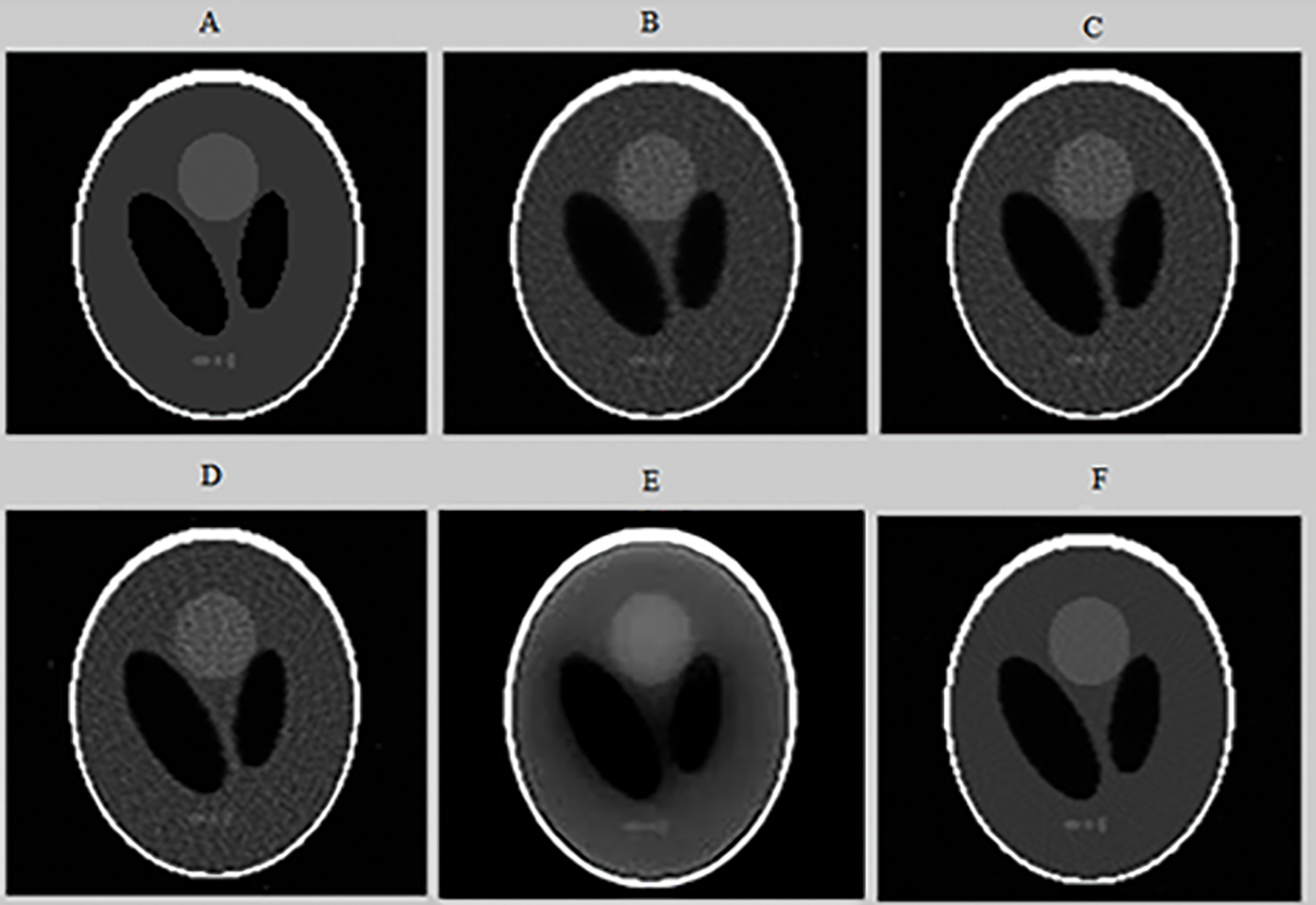
Figure 10: Axial slices of the tomographic Shepp-Logan Phantom (SLP) image reconstructed from noisy projections (projection 64) (A), using the following algorithms: 2D-MLEM (B), 2D-OSEM (C), 2D-OSEM with 3D-post filtering with a Metz filter (D), CNNR (E), and our proposed method (F)

Figs. 8 and 10 show that the proposed method allows the preservation of the original structure during reconstruction by removing noise and conserving contrast and details. Whereas the iterative method used alone (Figs. 10B and 10C) attenuates the detail by giving a blur effect on the edges of the areas and making the extraction and the location of the edges difficult. Likewise, the other improvement methods (Figs. 10D and 10E) affect the background uniformity. Subsequently, the image form appeared slightly smooth and noisy.

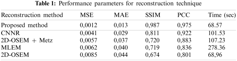
Fig. 11 shows the same profile of the Shepp-Logan slice reconstructed by the different reconstruction methods. The plot of the intensity profile shows that the profile resulting from the proposed algorithm (curve in pink color) is closer to the original profile (curve in green color) than the other algorithms. The other approaches provide either a more significant under-estimation or an over-estimation. This result demonstrates that the proposed method can efficiently recover the intensity of the original image compared to the other methods. In addition, quantitative analyses were used to evaluate the reconstruction methods. The optimum method has the lowest value of MSE, MAE and execution time and the highest value of SSIM and PCC. From Table 1, we note that the value of these metrics favored the proposed method which provides the highest value of SSIM (0.987) and PCC (0.975). This result demonstrates that the proposed method reconstructs a more similar structure than the other algorithms. Furthermore, the proposed method provides the lowest values of MSE (0.0012), MAE (0.013) and execution time (68.57) compared to other algorithms. This demonstrates that the proposed reconstruction algorithm preserves the edges and the quantitative information while removing noise. This method succeeds in keeping the compromise between noise reduction and details preservation. From this result, we can conclude that the proposed method ensures an accurate reconstruction in lower computational time compared to another algorithm.

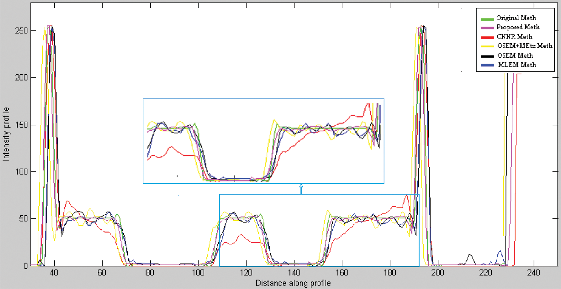
Figure 11: Line profile at row 35 of the noisy projections reconstructed respectively by MLEM, OSEM, 2D-OSEM with 3D-Metz post filtering, CNNR and proposed method applied

Axial slices reconstructed from a SPECT image of a Jaszczak by various reconstruction methods are shown in Fig. 12.

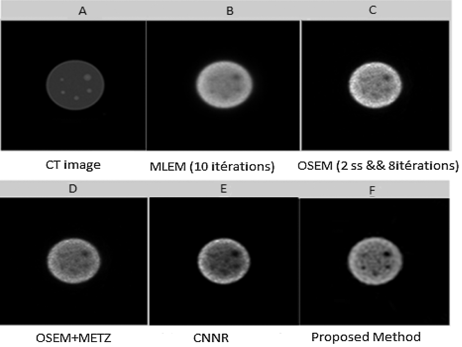
Figure 12: Axial slices (slice 73) reconstructed from the SPECT image of a Jaszczak phantom. (A) CT image; (B) Slice reconstructed by MLEM with 10 iterations; (C) Slice reconstructed by OSEM with (8 iterations and 4 subsets); (D) Slice reconstructed by OSEM with post-filtering by Metz filter; (E) Slice reconstructed by CNNR and (F) Slice reconstructed by the proposed method

From Fig. 12, it can be seen that the shape of the sphere seems more spherical and the background less uniform in the reconstructed slice with the proposed method. Whereas in the reconstructed slice with the other methods, the shape of the sphere seems slightly smoothed and attenuated, making the extraction and localization of the contours difficult and giving a much noisier image. This result shows the accuracy and efficiency of our proposed method in the reconstruction. It allows better preservation of detail and region boundaries than the other methods.

Figs. 13 and 14 show the results of CNR and SNR as a function of the Jaszczak phantom’s sphere diameters in slices reconstructed with the different reconstruction methods.

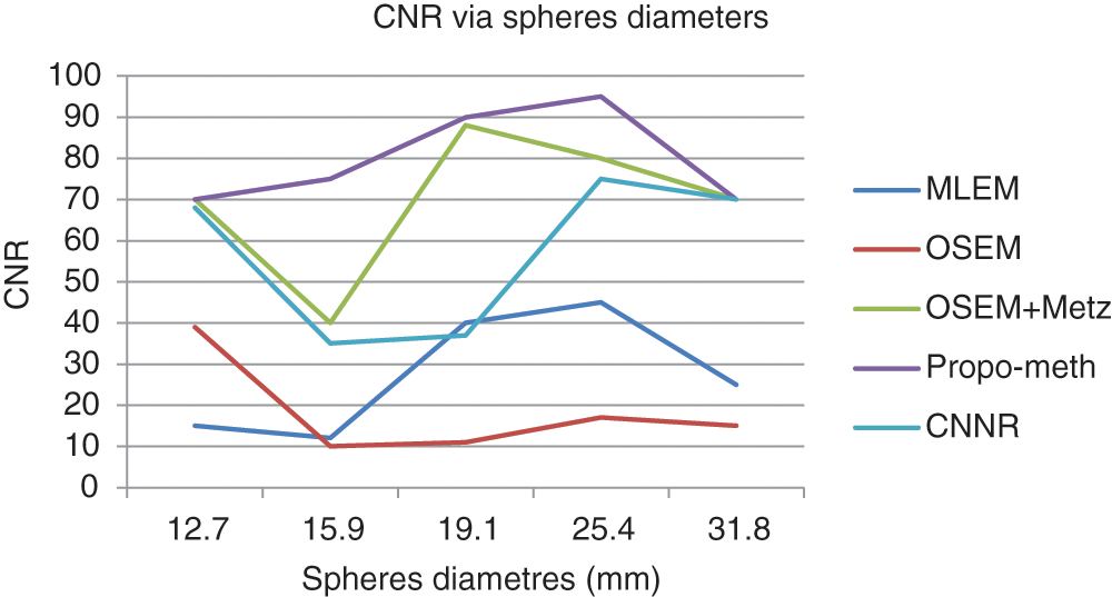
Figure 13: CNR according to the spherediameter of the Jaszczak phantom for the proposed method, OSEM, MLEM, OSEM + Metz and CNNR

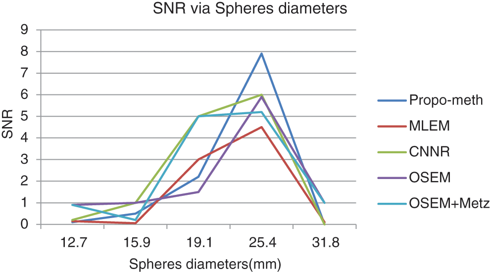
Figure 14: SNR according to the sphere diameter of the Jaszczak phantom for the proposed method, OSEM, MLEM, OSEM + Metz and CNNR

From Fig. 13, we can conclude that the CNR curves favor the proposed method over the other reconstruction methods. From Fig. 14, it can be seen that the images reconstructed by the proposed algorithm give better SNR values for spheres with diameters between 19.1 and 31.8 mm.

These curves illustrate that the proposed algorithm gives a better result for each metric than the other algorithms. This result shows the efficiency of our proposed algorithm in noisy artifacts reduction with conservation of contrast, improvement of SNR and image resolution.

The reconstructed bone SPECT image with: MLEM (120 iterations) (A), 2D-OSEM (8 iterations and 4 subsets) (B), 2D-OSEM (8 iterations and 4 subsets) with a 3D-post-filtering with a Metz filter (order = 9.5, FWHM = 7.8 mm) (C), CNNR (D) and the proposed method (E) are shown in Fig. 15.

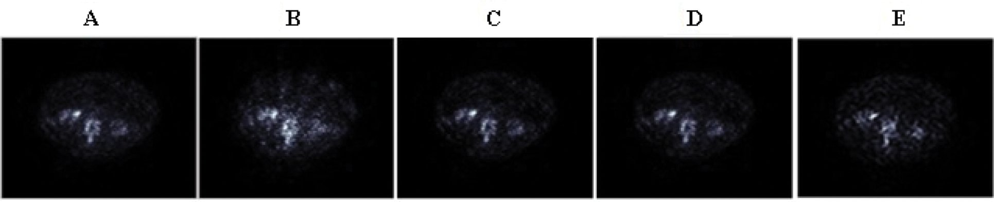
Figure 15: Axial slices of the clinical SPECT data, reconstructed by the five reconstruction algorithms

We can note from Fig. 15 that the anomalies and fine details become visible in the slice reconstructed with the proposed method. Moreover, we can see that the artifacts and undesirable activity in the background region, which is apparent in Fig. 15B, decreased with the preservation of image contrast.

For each method and each exam, we calculated the mean values of contrast, SNR and execution time for 31 bone SPECT exams described in Eqs. (9) and (10). Figs. 16–18 show the results of mean values of contrast, SNR and the execution time for 31 bone SPECT images.

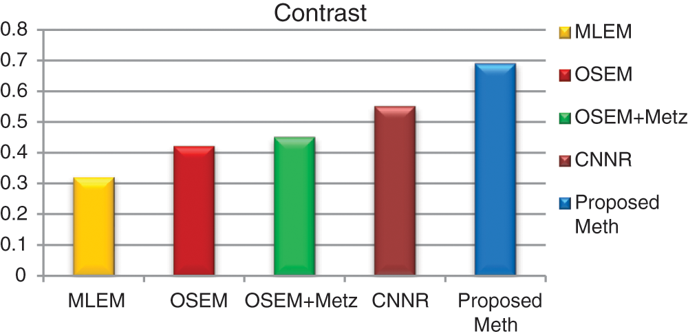
Figure 16: Bar plots of the means contrasts values, from different algorithms for 31 thoracic SPECT images

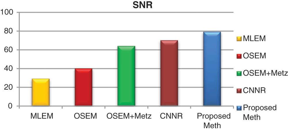
Figure 17: Bar plots of the means SNR values from different algorithms for 31 thoracic SPECT images

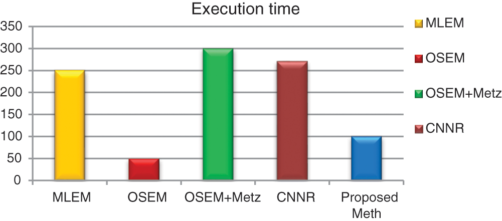
Figure 18: Bar plots of the execution time from different algorithms for 31 thoracic SPECT images as mean values

The qualitative assessment of the various directional feature regions of the bone SPECT image, illustrated in Fig. 15, shows that the proposed method provides better preservation of the singularity, the limit of the region, and more accurate detection of the lesion, and the practical ability of denoising. At the same time, the iterative method used alone attenuates the detail and makes delicate the extraction and the location of the contours.

For all the 31 thoracic SPECT exams, we can note from Figs. 16–18 that the proposed algorithm provides the highest values of SNR and contrast. The lowest value in terms of execution time compared to other methods illustrates the highest result. The execution time value of the reconstruction by the proposed algorithm is (100 ∓ 8.7 sec) outperform those by the other algorithms.

Using multi-scale denoising on the acquired bone SPECT projection images allows more considerable noise reduction with accurate radioactivity concentration and quantitative information measures. This technique is based on localized fine-scale functions, which allow better reconstruction of various details at multiple scales. Using the novel 3D-OSEM based on parallelization computation brings the convergence much faster than the traditional 2D-OSEM with robust and accurate reconstruction. The anisotropic diffusion is based on a nonlinear sigmoidal function, which generates various degrees of edge sharpening, accentuates and sharpens different details of the reconstructed thoracic SPECT image without affecting the neighboring regions’ background. In conclusion, this model allows a fast, robust and accurate reconstruction of thoracic SPECT exams.

As shown in Fig. 19, we have developed a graphical user interface to facilitate handling and display the desired slices according to the user’s choice.

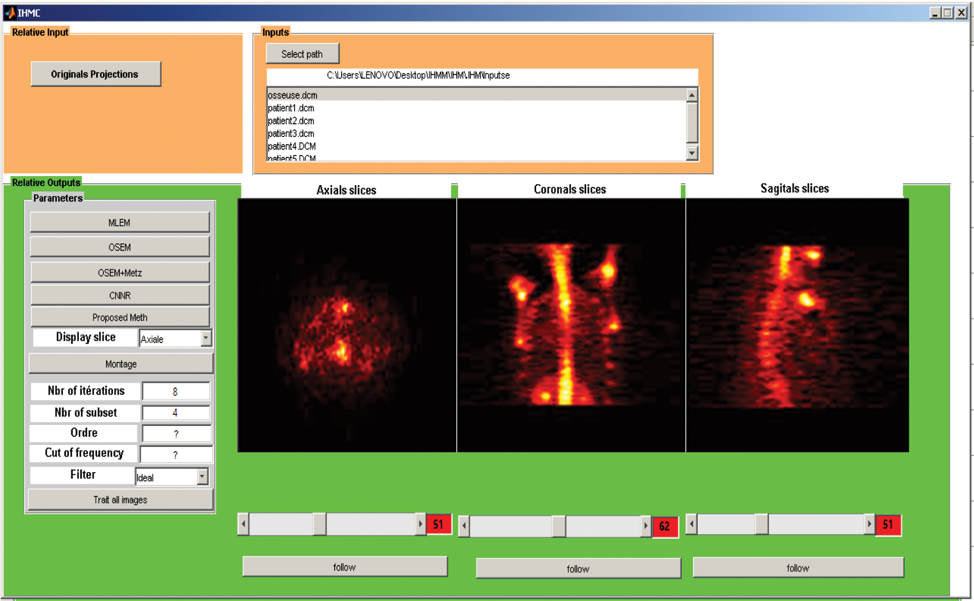
Figure 19: Graphical user interface of SPECT image reconstruction

4  Conclusion

In this paper, we presented a novel 3D algorithm to enhance bone SPECT image reconstruction. In fact, after applying a new type of filter exploring the possibility of combining two different multi-scale techniques, Wavelet transform and discrete Curvelet transforms, on 128 projections. One hundred twenty-eight axial slices are reconstructed by the 3D-OSEM algorithm and enhanced by one of the newest anisotropic diffusion models. The proposed method was tested on two different SPECT phantoms: Shepp-Logan phantom and Jaszczak phantom, and our bone SPECT database to demonstrate its accuracy and robustness in reconstruction. Summing up the results, it can be concluded that the proposed algorithm can improve the quality of thoracic SPECT images in terms of noise reduction, accuracy and reconstruction robustness. This novel method provides a notable gain, in contrast, SNR, CNR, MSE, MAE, SSIM, PCC and computation time compared to other algorithms. In this work, we proposed a user interface graphic for SPECT image reconstruction that allows the practitioner to correct the spatial resolution of the bone in SPECT image. A limitation of this study is that the parameters of this algorithm are chosen according to the statistic study carried out and the database used. Based on the promising results presented in this article, we propose a combination of this algorithm with a deep learning method as a possible direction of research in the future to obtain an optimal and innovative method of bone SPECT image reconstruction.

Funding Statement: The authors received no specific funding for this study.

Conflicts of Interest: The authors declare that they have no conflicts of interest to report regarding the present study.

This work is licensed under a Creative Commons Attribution 4.0 International License, which permits unrestricted use, distribution, and reproduction in any medium, provided the original work is properly cited.