| Computer Modeling in Engineering & Sciences |
DOI: 10.32604/cmes.2022.018544
ARTICLE
Peridynamic Modeling of Brittle Fracture in Mindlin-Reissner Shell Theory
1Department of Engineering Structure and Mechanics, Wuhan University of Technology, Wuhan, 430070, China
2Hubei Key Laboratory of Theory and Application of Advanced Materials Mechanics, Wuhan University of Technology, Wuhan, 430070, China
3State Key Laboratory of Advanced Technology for Materials Synthesis and Processing, Wuhan University of Technology, Wuhan, 430070, China
*Corresponding Author: Xin Lai. Email: laixin@whut.edu.cn
Received: 01 August 2021; Accepted: 29 December 2021
Abstract: In this work, we modeled the brittle fracture of shell structure in the framework of Peridynamics Mindlin-Reissener shell theory, in which the shell is described by material points in the mean-plane with its drilling rotation neglected in kinematic assumption. To improve the numerical accuracy, the stress-point method is utilized to eliminate the numerical instability induced by the zero-energy mode and rank-deficiency. The crack surface is represented explicitly by stress points, and a novel general crack criterion is proposed based on that. Instead of the critical stretch used in common peridynamic solid, it is convenient to describe the material failure by using the classic constitutive model in continuum mechanics. In this work, a concise crack simulation algorithm is also provided to describe the crack path and its development, in order to simulate the brittle fracture of the shell structure. Numerical examples are presented to validate and demonstrate our proposed model. Results reveal that our model has good accuracy and capability to represent crack propagation and branch spontaneously.
Keywords: Peridynamic; brittle fracture; Reissner-Mindlin shell theory
Dynamic damage and failure process of shell structure is very challenging in the computational community for its special geometric features which requires the numerical method to be capable of representing material characteristics and discontinuity in finite deformation and large rigid rotations [1]. Because the intrinsic nature of the discontinuities emerges from the damage area of interest, numerical approaches based on classical continuum mechanics have to handle the discontinued displacement field and the singularity in stress field at the crack tip, where partial-differential equations become unsolvable. Instead, the peridynamic theory provides a uniform description of both continuities and discontinuities, which reform continuum mechanics by providing a non-local integral representation of continuum material and structure responses [2]. There is no requirement for the continuity of the displacement field since the domain is discretized in terms of material points and described by the integral equation of motion. The cracking and failure can thus be captured and represented naturally and spontaneously without artificial treatment or additional criterion.
Peridynamic theory has been proposed by Silling in 2000 and it has been successfully applied to solve problems in engineering and industry with material damage and fracture involved [3–5]. Chu et al. then proposed a modified bond-based peridynamic model which considers the softening plasticity in compression and strain-rate effect of ceramics [6]. Chen et al. developed a peridynamic fiber-reinforced concrete model based on the bond-based peridynamic model with rotation effect [7]. Bazazzadeh et al. study fatigue crack propagation in structural materials by developing a new computational tools which is based on peridynamic theory [8, 9]. Zhao et al. presented a state-based peridynamic contact damage model for glass by introducing a contact force function [10].
However, when it is extended to plate or shell structures, it is very hard to achieve reasonable results with high accuracy since the system have to use very fine discretizations to satisfy the precision requirement along the thickness direction. To address this issue, several peridynamics membrane approaches have been proposed based on various kinematic assumptions to improve the computational efficiency [11 –13]. A new notion of curved bonds is exploited to cater for force transfer between the peridynamic particles describing the shell structures firstly by Chowdhury, et al. [14]. Recently, a PD model for 3D shell structures with six degrees of freedom to predict the damage and crack growth developed by Nguyen et al. [15]. Hu et al. present a methodology for the simulation of ductile fracture in steel plates based on non-ordinary state-based peridynamics [16], which also provide a novel algorithm of crack approximation. Yolum reduces the number of peridynamic interactions by idealizing the plate structures with mindlin plate theory [17], obtained a peridynamic solution for elastic deformations and failure prediction of pre-cracked plates. In fact, the possibility to model these structures with a single layer of nodes is very attractive. The same conclusion was drawn concerning other meshfree particle methods for ages. In 2000, Li et al. presented an meshfree simulations of large deformation of thin shell structures by constructing highly smoothed shape functions for three-dimensional meshfree discretization [18], while avoiding ill-conditioning as well as stiffening in numerical computations. A method relies on an entirely meshless based on the Smoothed Particle Hydrodynamics method (SPH) presented by Maurel et al. [19], and discussed the simulation of a plasticity model of the thin shell and its fracture analysis. Lin et al. modified the Smoothed Particle Hydrodynamics method (SPH) to deal with shell-like structures with only one layer of particles to represent the shell mid-surface [20], while keeping a very good level of validity and efficiency. Peng et al. developed the Reproducing Kernel Particle method (RKPM) to the simulation of the large deformation of a curved shell in the Mindlin-Reissner shell theory [21], which can address large deformations without mesh distortion. By using this method, the dynamic response of the ship cabin and real ship structure under impact load are numerically predicted [22]. Zhang et al. derived the local form of nonlocal balance laws for nonlocal continuum and developed a nonlocal geometrically-exact shell theory. The finite deformation and fractures are simulated by that model [23]. Yang et al. used Lagrange’s equation and Taylor expansion to update the motion equation and develop the new state-based peridynamic formulation for functionally graded Euler-Bernoulli beams with four different boundary conditions considered [24]. Shen et al. present new peridynamic beam and shell models with the effect if transverse shear deformation based on the micro-beam bond and the Timoshenko beam theory [25] and the crack propagation in double-torsion test of a rectangular brittle plate has been simulated [26].
This paper is organized as follows. In Section 2, we first recall the Mindlin-Reissener shell theory, and we introduce the numerical instability control to eliminate the zero-energy mode and rank-deficiency. Then the details of brittle fracture modeling and crack criterion are proposed. After that, some elastic numerical examples will be provided to illustrate the capabilities of this theory. In Section 3, numerical examples are carried out to validate the accuracy, investigate the convergence, and demonstrate the capability of proposed model on brittle fracture modeling. studies the damage theory and the crack simulation algorithm. Finally, the accuracy, convergence, and stability of this work will be discussed in the last section.
2 Modeling Brittle Fracture in Mindlin-Reissner Shell
2.1 Non-Ordinary State-Based Peridynamic Theory
The Non-Ordinary State-Based Peridynamic Theory is a non-local continuum theory that was proposed by Silling [27], in which the interactions between material points are measured in terms of force states. Each pair of interactions between material points are arbitrarily oriented and magnituded. The governing equations of the linear momentum of the system is expressed as
where ρ0 is the mass density at the initial configuration, : x denotes the position of the material point in the body, : u(: x, t) is the displacement of : x at time t, : b is the body force density, and
Eq. (1) could be seen as an non-local form of the equation of linear momentum in continuum mechanics, which is
where : P is the first Piola-Kirchhoff (PK-1) stress tensor, and ∇X is the divergence operator with respect to the initial configuration. In non-ordinary state-based Peridynamics, the force state
in which
where ξij = : xj − : xi, and : xi is the position vector of point i in the reference configuration.
2.2 Peridynamic Formulation of Mindlin-Reissner Shell
According to the Mindlin-Reissner’s thick shell theory, the shell is modeled using a single layer of particles that having three degrees of freedom in translation and two additional rotational degrees of freedom θ1 and θ2 in the plane tangent to the shell. Drilling rotation is not considered in this context for simplicity.
In Fig. 1, the kinematic interpretation of arbitrary shell is presented. The position vector of any point located at a distance η from the mean plane in the reference configuration can be expressed as
where

Figure 1: Kinematic description of Mindlin-Reissner shell
At the mean plane of the shell, any point that belongs to the parametric space
where : E1 and : E2 are the basis vector in the parametric space. To better describe the motion of the shell, we define the convected basis vectors : G in the reference configuration as
in which : T is the pseudo normal vector, which is also referred as “fiber” in many literatures [28]. In Mindlin-Reissner shell theory, the shear deformations through the thickness of the plate is considered comparing to Kirchhoff-Love theory. The fiber or pseudo normal of the shell represents the normal of the mid-surface, and it will keep straight but not necessarily perpendicular to the mid-surface after deformation. For any point on the mean plane of the shell, one can always find a local coordinates system described by : G1, : G2, and : G3. In the following context, we assume that by adopting appropriate basis : Eα in the parametric space the local coordinates at : x can be made orthogonal.
Now we consider the position of a point in the current configuration with a motion χ respect to the reference configuration. The position vector of any point can be expressed as
where : T(ξ1, ξ2) indicates the pseudo normal vector in current configuration that is mapped from parametric space, and ϕ(ξ1, ξ2) defines the mid-plane of the shell in current configuration.
Similarly, we defined the convected basis vectors : G in current configuration are defined as
where : T denotes the pseudo normal vector along the fiber direction at current configuration. One may readily get the displacement of each point by
where : u(ξ1, ξ2) is the displacement of point on the mean plane of the shell in the current configuration. Given the above definition we note that : T(ξ1, ξ2) and : T(ξ1, ξ2) is the mapping from position of point we interested in the parametric space to the pseudo normal vector in initial or reference configuration, which is
To further simplify the computational process and clarify the constitutive updating objectivity, we introduce the rotation matrix : R0 which transfer the position vector in the initial/reference configuration from the global coordinates : x to the local coordinates : xl, such that
If the mean plane of the shell is flat and lies on the XOY plane in the initial/reference configuration, one can simply set : R0 = : I. Since fiber is initially perpendicular to the mean plane of the shell, one could find : xl3 = : T.
Likewise, we also define a rotation matrix : R which evolves with time that transfer the position vector in the current configuration from the global coordinates : x to the local coordinates : xl, such that
The motion χ from the initial configuration to current configuration could be seen as the combination of two motions, i.e., from the parametric configuration to the reference configuration Φ0, and from the reference configuration to current configuration Φ. Then we can write deformation gradient for χ as
Using chain rule, following relation could be reached
where ∇ξΦ and ∇ξΦ0 is the deformation gradient of motion Φ and Φ0 relative to the parametric configuration, respectively. Recall the equivalent non-local material differential operator defined as follows
where
where
Note the deformation gradient motion of Φ and Φ0 in terms of the convective coordinates are given by
The deformation gradient for three motions Φ, Φ0, and χ can then be written in matrix form as follows:
and,
in which ξα = ξα , α = 1, 2.
The in-plane tangent convected vector : gα could be updated by
Also, one can readily have
which implies that the pseudo normal vector in the mean plane of the shell at current configuration could be updated by the following relation:
and,
which may not parallel to the normal to the tangent plane of the mid-surface.
2.4 The Pseudo Normal Vector Updating
In this work, we use the Euler-Rodrigues rotation formula to update the direction of fibers. The pseudo normal vector : T is related to its initial state : T under assumption of a smooth motion by
where : R is the rotation matrix which could be evaluated in each time integration.
in which : I is the identity matrix, and θ is the magnitude of rotation vector
and,
Taking time derivative of Eq. (28), consider that : T in referene configuration is independent with time, we can obtain
where ω is the angular velocity, which is an axial vector correlated with the skew-symmetric tensor Ω which satisfy
One could obtain the strain based on the deformation gradient under finite deformation and rotation. The spatial velocity gradient could be obtained by using the following relationship:
where
in which
where we have used the nonlocal convective gradient operator again,
Then the spatial velocity gradient could be decomposed into stretch and skew part
where : d and ω are the rate of stretch and rotation tensor, respectively.
From the non-local deformation gradient, one can obtain the Green-Lagrangian strain tensor by
where : c is the right Cauchy-Green deformation tensor with : c = : FT: F.
The the Eulerian-Almansi finite strain is given by
where : c is the finger tensor defined by : c = : F−T: F−1
The Eulerian-Almansi strain could be transfered from the Green-Lagrangian strain by
To further facilitate the plane stress hypothesis, the constitutive equation is evaluated in the local coordinate system. The Eulerian-Almansi strain is first transformed into the local system by an orthogonal tensor : Q
Using Voigt’s notation, the Almansi strain tensor in local system and the Cauchy stress tensor in local system could be expressed in vector form by
Utilizing the plane stress hypothesis, the component along the direction of plane thickness is zero, which yields
If the material is assumed to be elastic, reduced constitutive equation proposed by Hughes [29] is adopted to obtain stress state from strain,
where E is the Young’s modulus, ν is the Poisson’s ratio, and κ is the shear correction factor. If the thickness variation is considered, ɛ33 should be calculated within the constitutive model to satisfy the zero normal stress condition σ33 = 0. Once the Cauchy stress being obtained in the local coordinate system, we transform it into global coordinate
where σl is recovered from local Cauchy stress vector in Voigt’s notation. The first Piola-Kirchhoff stress in total Lagrangian formulation can be obtained in the global coordinate system,
2.6 Governing Equations for Linear Momentum and Angular Momentum
In current work, the balance laws and nonlocal governing equations for Peridynamic shells proposed by Zhang et al. [30] are adopted to describe the material in the system. The linear momentum of the Minlin-Reissner shell in non-local form at the mean plane satisfies the following governing equation:
in which h is the initial thickness of the shell, ϕ is the motion of the point at the mean plane at time t, : xi is the spatial position vector of particle i in the parameter space,
and,
where Ψ is the stress resultant that is expressed as
where
The angular momentum balance of equation of the shell is governed by
where : T is the pseudo normal of the orientation of the fiber at current configuration, and
and,
where Πi is the momentum stress resultant as expressed as
2.7 Numerical Instability Control
In non-ordinary state-based peridynamic theory, one may expect the so-called zero-energy mode, in which multiple deformation states could be related to the same unique deformation gradient, caused by the averaging of the kinematic information of all neighboring particles around one material point. It will introduce spurious nonphysical oscillations of stress, strain, and displacement field in the domain, which consequently may lead to system instability and inaccurate predictions, especially for transient and finite deformation problems.
Many pioneer work have been reported to try to address this problem from different aspect. In classic Finite Element Method, Hughes and Liu tried to eliminate the appearance of zero-energy in-plane rotational modes by using “Heterosis elements” [28], in which more gauss point was used to evaluate the bending of the plate. For Smooth Particle Hydrodynamics (SPH) implementation of Mindlin-Reissner shell, similar treatment was reported and practiced by Maurel and Combescure [19]. For Peridynamics, Littlewood proposed a penalty approach to mitigate the zero-energy modes [31], where a hourglass force is added to help eliminating spurious solutions. Breitenfeld considered three methods of zero-energy mode control [32], including supplemental interconnected springs, average displacement state, and penalty approach. Stability method is then suggested by Silling [33] and extended by Li et al. [34, 35], where additional term is added to the strain energy density that resists zero-energy mode of deformation. Other treatment includes sub-horizon or bond-associated deformation gradient [36, 37], stress-point method [38, 39], etc.
In current work, we use the stress point method to reduce the rank-insufficient induced numerical divergence and oscillations. Stress points are added into the domain to help increasing the stability, as illustrated in Fig. 2.

Figure 2: Illustration of stress point setup
The four particles points on the middle surface(lamina surface) of the shell form an integral element. Arrange a stress point in the center of the integral element, shown in Fig. 3. Considering the integral in the thickness direction of the shell, each integral element corresponds to an integral cell, in Fig. 3b. In this way, the shell is discretized into integral cells with thickness. The function value of each stress point can be obtained by integrating the value obtained in the integration cell. Therefore, the Gaussian points are arranged perpendicular to the centerline of the grid in the lamina surface and its number can be determined according to the accuracy requirements. For this work, we choose three Gaussian points for each integral cell.

Figure 3: Gaussian integration domain
In the calculation, the integral value corresponding to the Gauss point is obtained by integrating on the integration plane where the Gauss point is now, and then integrating through the line distribution of the Gauss point in the normal direction, and the obtained value is used as the corresponding function value of the stress point.
Each stress point have its own horizon in which it interacts with its neighboring material points within a certain range. The deformation gradient at the stress point is obtained by interpolation of the deformation gradient on its neighboring material point family. Stress is obtained from strain and constitutive relationship at the stress points, and then interpolated back to the material points. The computational scheme of the physical properties on the stress points and the material points is given as follows:
where φj and : Fsi represent the coordinate and the deformation gradient of material points, respectively.
In conventional Peridynamic theory, bond-breaking is mainly driven by the stretch of the bonding between material points, that when the bond stretch limit was met, the bond will break spontaneously, which in turn accumulated to shape the crack surfaces. However, if a correspondence material model is utilized to describe the material response, such as plasticity, the bond-breaking criterion needs to be modified to represent the fracture properties of the material.
In current work, the Mohr-Coulomb failure criterion is adopted as the principle of bond-breaking, in which the principle stress state are used to determine the material failure, and the tension and compression could be treated separately. When such criterion being satisfied at the stress point in the domain, we treat it as fully damaged, thus any stress points that sharing the same fiber will be considered as fractured.
Under such consideration, the damage state is assumed to be initialized and propagate at the stress point of the shell, which means that cracking is realized by nucleating and extending cracks between damaged stress points. This approach of fracture modeling will surely introduce additional work to maneuver the initialization, propagation, and branching of the cracks, which need to book-keep the historic information of the crack surfaces. The Peridynamic bonding between material points will then be cut by the forming and propagating crack surfaces, which will then in turn represent the material failure in manner of material points.
2.8.2 Cracking Surface Tracking
The crack surface is composed of segments connected by stress points. Since the shell is represented by the material points at the mean plane, we only consider cracks running inside the mid-surface of the shell, and when certain spot of the shell being cracked, the crack go through the thickness direction which is denoted by the pseudo fiber oriented at the parametric space. In other words, when stress points that share the same pseudo fiber along the thickness direction get to a accumulated state of complete damage, the whole shell section where the stress point resides is considered to fail immediately. A new crack tip will then be generated at the stress point and thus forming the new crack surface, as illustrated in Fig. 4, in which, new crack tip that created at stress point B will connect with original crack tip at stress point A to create new crack surface AB. The new crack surface will cut any connection between stress points and material points or those between material points, e.g., AB will break the connection between stress point D and material point C3.
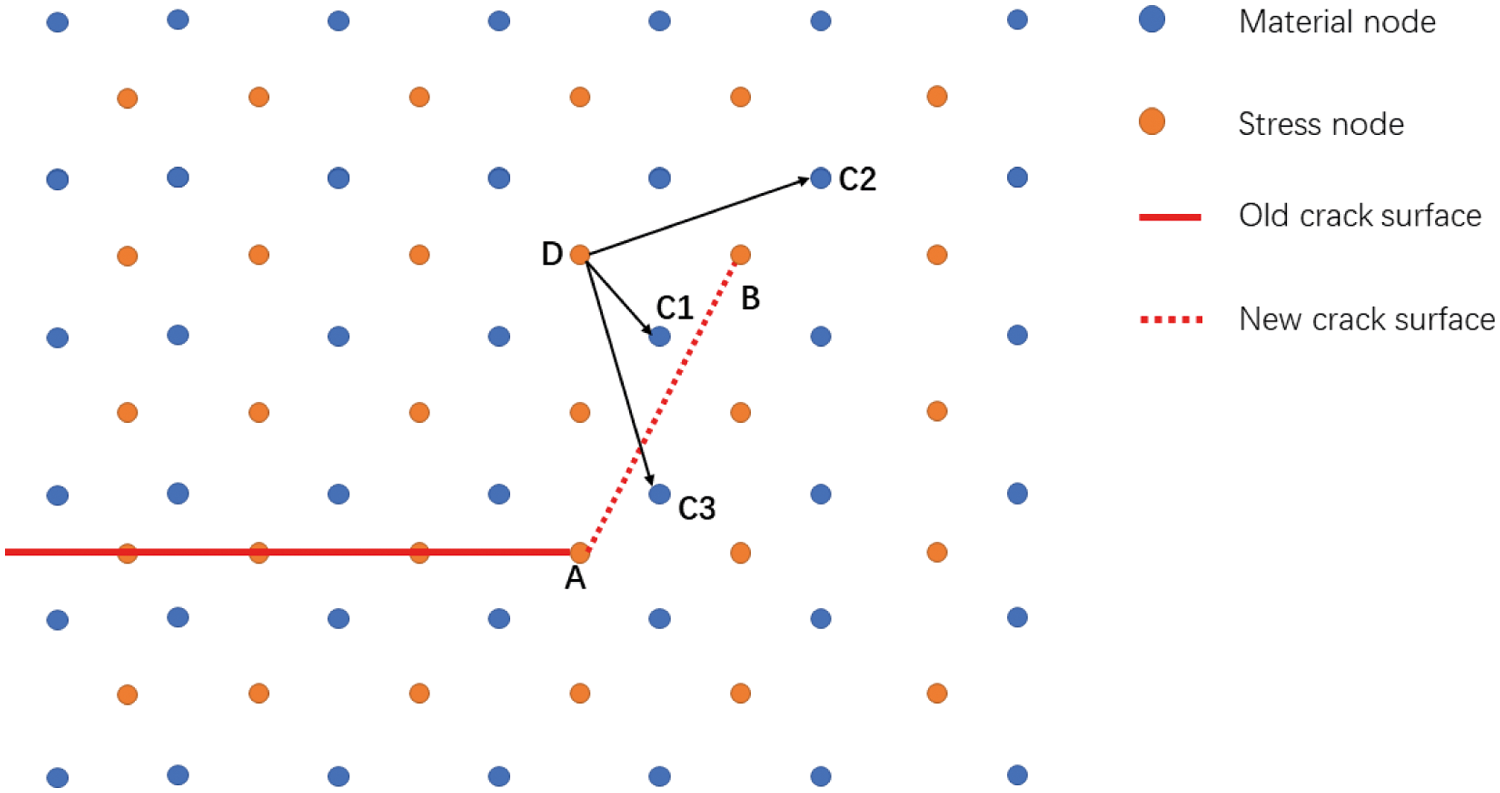
Figure 4: Crack surface and visibility condition of shell
When the bond-breaking criteria are met, new crack tip will be generated. If there are multiple spots of the stress points satisfy the criterion, that have the largest magnitude will be chosen as the new crack tip with other candidates remain intact.If the newly nucleated crack tip is the only one in the shell, or it does not belongs to any existing crack surface, i.e., it is far away enough from all cracks in existence, we marked it the nucleation of a new crack surface. Otherwise, we evaluate the existing crack surfaces and pick one of them, from which the new crack tip has the nearest distance from. The new crack tip will be added to the surface of the chosen crack path, which then expands from the old crack tip to the new one. Hence a new crack surface segment is created. Each time new crack surfaces are developed, we need to do bond-breaking of the material points by apply crack surfaces to the connections of all the bondings. If by any chance, when new crack tip being created, we divide material points, if any, that are exactly located on the formed crack surfaces geometrically, into two. A tiny gap δ(δ < < 1) relative to the normal direction n1 of the crack surface will be added to separate the two consequential material points. The normal direction of the crack can be obtained from the normal direction of the shell at the position of the stress point at the old crack tip and the relative coordinate vector of the stress point at the new and old crack tip, as
in which : E3 is the shell normal direction at the tip of the old crack. And xon is the relative coordinate vectors of new and old crack tips.
The resulting two material points bisect the mass and volume of the original material point, and inherit all other properties of the original material point, including linear velocity, linear acceleration, angular velocity, angular acceleration, translational displacement, and rotation angle. The newly generated crack surface can be projected back to the parametric space, in which the crack discontinuity plane in 3D is represented by a planar line. The bond-breaking process is handled in parametric space, which can take advantage of simplified geometric information.
In this work, the crack surfaces will break both the connection between stress points and material points, and those between material points themselves. The former one we already discussed in beginning of this section. For the bond-breaking between material points, the problem is simplified to whether two line segments intersect with each other, as illustrated in Fig. 5. When the new crack surface being created by connecting the old and new crack tip A and B, the bond between material points C and D will be broken if the two line segments have point of intersection, i.e.,
in which : n1 and : n2 are the normal direction of the line segments AB and CD, respectively, that can be obtained by using Eq. (63). : xCA = : xA − : xC denotes the relative line segment vector in parametric coordinate space.
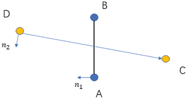
Figure 5: Schematic illustration on cracking criterion
2.8.3 Crack Simulation Algorithm
During the calculation, it is first necessary to solve the damage situation of the stress point. According to the Eqs. (50) and (60), the damage of the stress point needs to be obtained by integrating the integration domain to which the stress point belongs. The Gaussian points of the integration domain is complete damage when the stress satisfies the Mohr-Coulomb failure criterion and Dg = 1.0. The damage of the Gaussian points could be calculated by
Due to the geometric characteristics of the shell, our work does not consider the evolution of the crack in the thickness direction of the shell, which means the crack always penetrates the thickness direction of the shell instantaneously. Thus, if the damage of the stress point is larger than the limited damage Dlimit, the stress point is been a new crack node.
As shown in Fig. 6, if a new crack node appears in a certain range around the crack tip of an existing crack which is been called the crack domain (
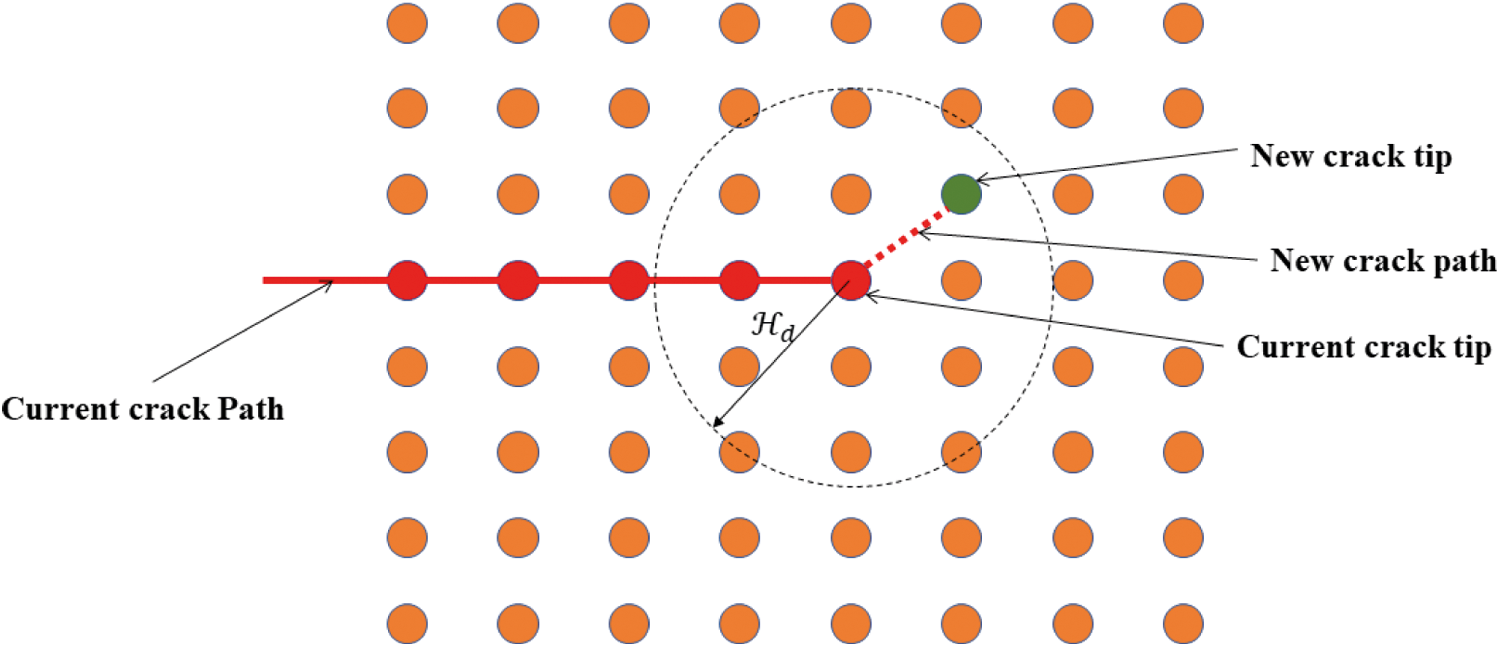
Figure 6: Crack extension
As shown in Fig. 7, if a new crack node appears in the crack domain of any one or more existing crack nodes on an existing crack, a new crack will be formed from this new crack node to the existing crack node with the shortest distance from it. The macroscopic manifestation of this process is the main crack bifurcation.
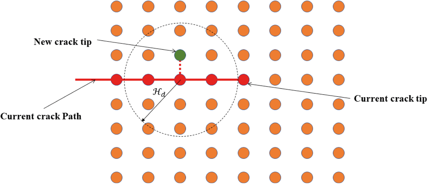
Figure 7: Crack bifurcation
As shown in Fig. 8, if the new crack node is not in the crack domain of any existing crack, the crack node is considered to be the starting point of the new crack, but it does not affect the structure and materials.
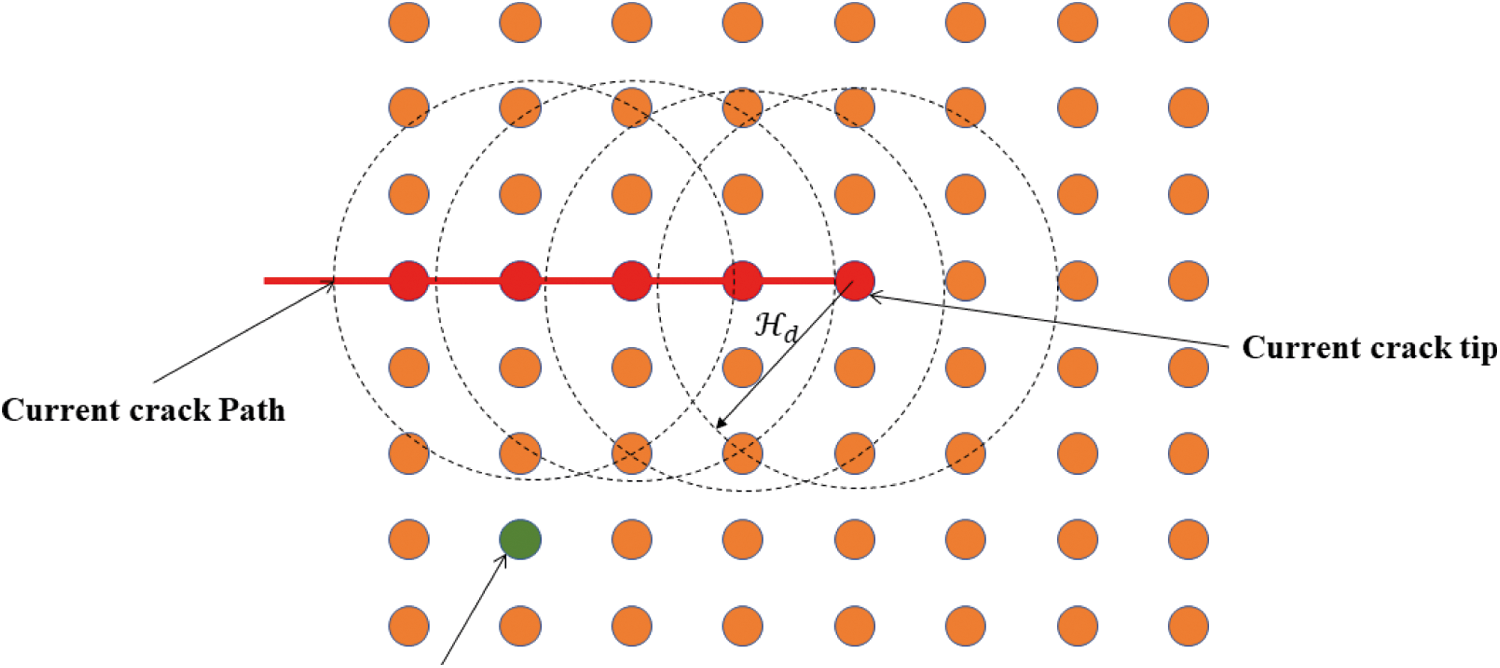
Figure 8: Crack initiation
The formation of new crack surfaces will affect the interaction between particles. This process is called bond breaking. Similarly, the corresponding relationship between the stress point and the particle will also be separated by the crack surface, too. It can be judged by the simplified visibility condition mentioned above. When the relationship between any points A and B is interrupted by the crack surface, the displacement state of one point will no longer affect the other point. The relative position between them remains unchanged at the moment the key is broken. Therefore, as the crack grows, the particles around the crack are affected by the crack, but the neighboring particles remain unchanged. When solving the shape matrix K, there is no need to update the neighbors. The pre-crack is set on the geometric model in the initial step of the calculation, and thereafter, it will always exist in the model as the current crack. The flow chart of the crack simulation algorithm is illustrated in Fig. 9.
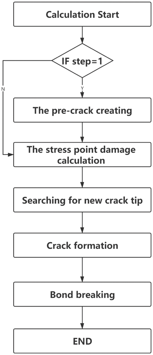
Figure 9: Flow chart of crack simulation algorithm
In this section, several numerical examples are used to validate and demonstrate the validity of our implementation and capability of the proposed approach. The first two numerical cases are aimed to verify the validity and the accuracy of our implementation of the Peridynamic shell. The latter two cases are carried out to explore the capability of our model on representing the dynamic fracture of the shell.
3.1 Elastic Case 1: Clamped Plate Under Uniform Pressure
In this section, the square clamping plate with side length L = 0.5m and thickness h = 0.1m is numerically modelled before being subjected to a uniform pressure of P = 1MPa. The material of the plate is elastic, with mass density ρ = 7850kg/m3, elastic modulus E = 2.1×10¹¹Pa, and Possion’s ratio ν = 0.3. The pressure is applied at the beginning of the simulation and maintain its value throughout the computation process. The schematic diagram and the geometric information of the plate are illustrated in Fig. 10, as well as the material parameters. The dynamic response of the plate is analyzed to verify the convergence and accuracy of the present method in dynamic simulation.
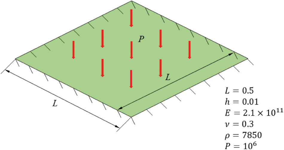
Figure 10: Schematic illustration of the geometry and setup for clamped plate
Three different numerical discretizations are used to obtain the dynamic responses of the plate, which are 6 × 6, 11 × 11, and 21 × 21, respectively. The horizon δ is chosen to be the same with the particle spacing Δ x. After numerical simulations, the results are compared to those obtained by commerce FEM software package ABAQUS with a model consisting of 64 × 64 elements to validate current Peridynamic implementation. The vertical displacements of the central point of the shell from both Peridynamic and FEM results are given in Fig. 11. One can find that the numerical solution by the current Peridynamic model converges to FEM solution quickly as the discretization increases. The time sequence of the deflection of the plate is illustrated in Fig. 12, in which the deflection has been vertically amplified 10 times to show the deformation, and the material points are colored by the vertical displacement. We can find that the material points are smoothly distributed with no instability, which indicates that the rank deficiency is eliminated effectively with the stress point technic.
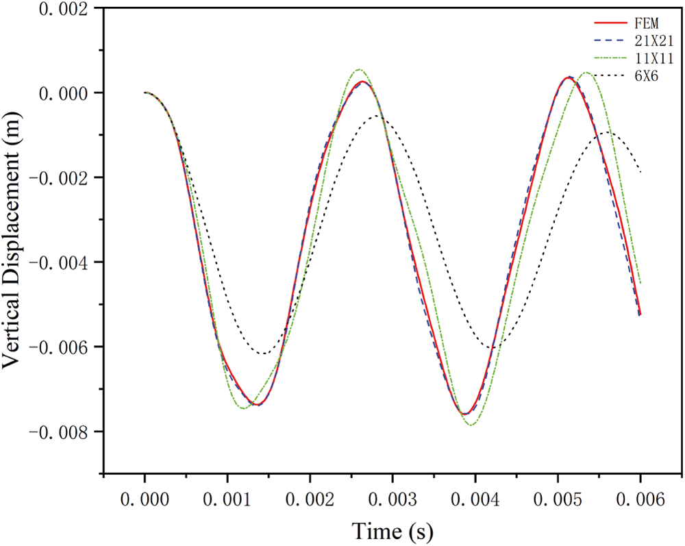
Figure 11: Evolution of the vertical displacement compared with results obtained from ABAQUS

Figure 12: Time sequence of the deflection of the clamped plate(× 10)
3.2 Elastic Case 2: Scordelis-Lo Roof
In this section, we present a numerical example of the scordelis-Lo roof, a cylindrical segment under gravity, as shown in Fig. 13. The curved edges are simply supported, and there are no constrains on the other two edges. Four different numerical discretizations are considered to investigate the δ convergence of the numerical example. The free edge of each quarter of the shell are consisted by 5, 10, 12, and 17 material points, respectively. The vertical displacement of the midpoint of the side edge is measured as the vertical deflection of the shell to evaluate the accuracy and convergence of the system. It is first normalized by the reference value 0.3024m suggested by Scordelis et al. [40] before plotted in Fig. 14. From the comparison with results from Belytschko’s [41] and Simo et al. [42], we can find good agreement in aspect of the deflection, with reasonable spatial convergence rate as we refine the discretization of the system. We also compare the distribution of the vertical displacement of the roof with the results obtained by FEM. Reasonable agreement could be found, as illustrated in Fig. 15, in which there are 17 material points of each side for the Peridynamic model and 34 elements for the FEM model.
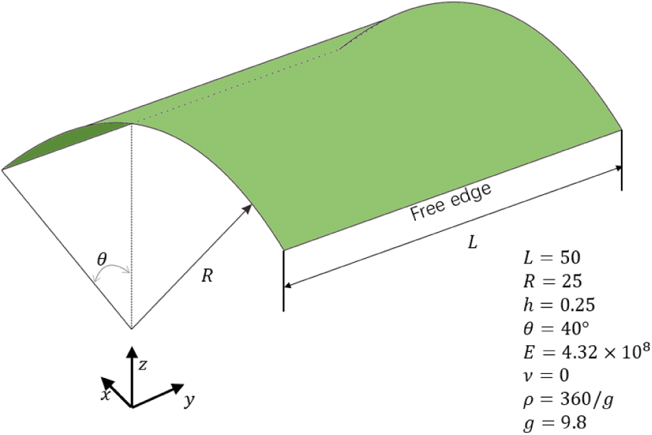
Figure 13: Schematic illustration of the geometry and setup for Scordelis-Lo roof
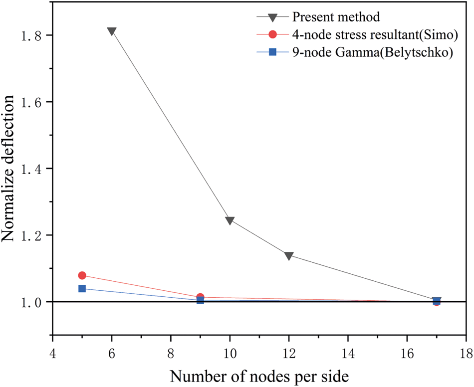
Figure 14: Convergence of the normalized deflection
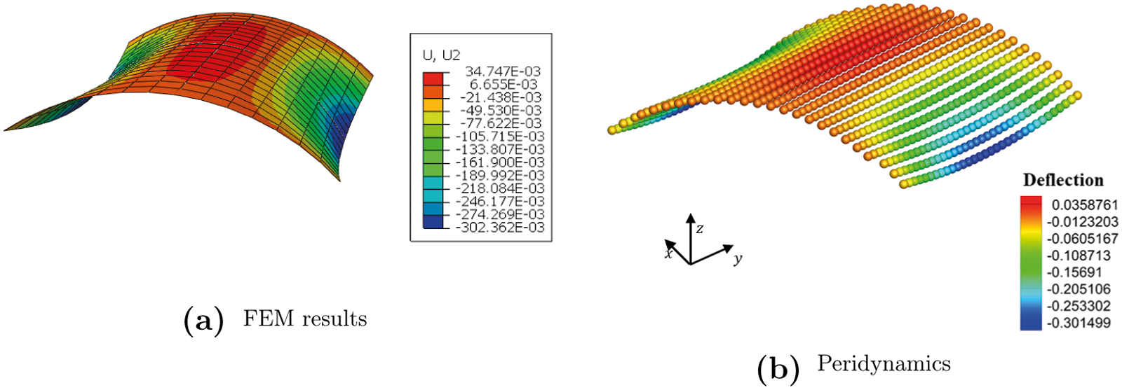
Figure 15: Deflection of the Scordeli-Lo roof under gravity(×10)
3.3 Fracture Case 1: Crack Predicting and Crack Branching in Brittle Material
In this section, a dynamic fracture of the brittle plate is numerically modeled and simulated. A rectangular plate with a pre-notch under symmetric tensile loading is considered, as shown in Fig. 16. A sample with dimensions 10 cm by 4 cm, is used to investigate the effects of loading conditions. The external loads are suddenly applied and maintained constant afterward. The mechanical properties of the material are chosen with elastic modulus E = 32GPa, mass density ρ = 2450kg/m3, and Poisson’s ratio μ = 0.22 [43]. In this work, the Mohr-Coulomb failure criterion is considered. And the compressive strength and tensile strength are σc = 32Mpa and σt = 2.07Mpa, respectively. The maximum principal stress failure criterion is adopted as the cracking criteria in this case. A step loading σ = 1.0MPa is symmetrically applied on the upper and lower boundaries of the plate at the beginning. A dynamic explicit time integration scheme is adopted, and the crack propagation process is visualized and plotted in Fig. 19. It is then compared with experimental data, illustrated in Fig. 17 [44], and the XFEM result by song et al. [43]. It can be observed that the crack propagates initially along the centerline, and eventually branches towards the edge of the plate. By the comparing our results with experimental and numerical references, reasonable agreement could be established between the predicted crack growth path and the experimental observation, which demonstrates the capability of predicting the dynamic brittle fracture of shell structures. We need to emphasis that although we are using the same geometry and loading condition with other numerical investigators [43 , 45, 46], the cracking in our study is predicted in a 3D thin shell, which have non-negligible difference with other numerical studies that use 2D model. Nevertheless, the criteria for the crack propagation is distinctive from the standard peridynamic theory to match up the stress point method, which is believed to be the reason for the trivial diversity between our crack paths with the references.
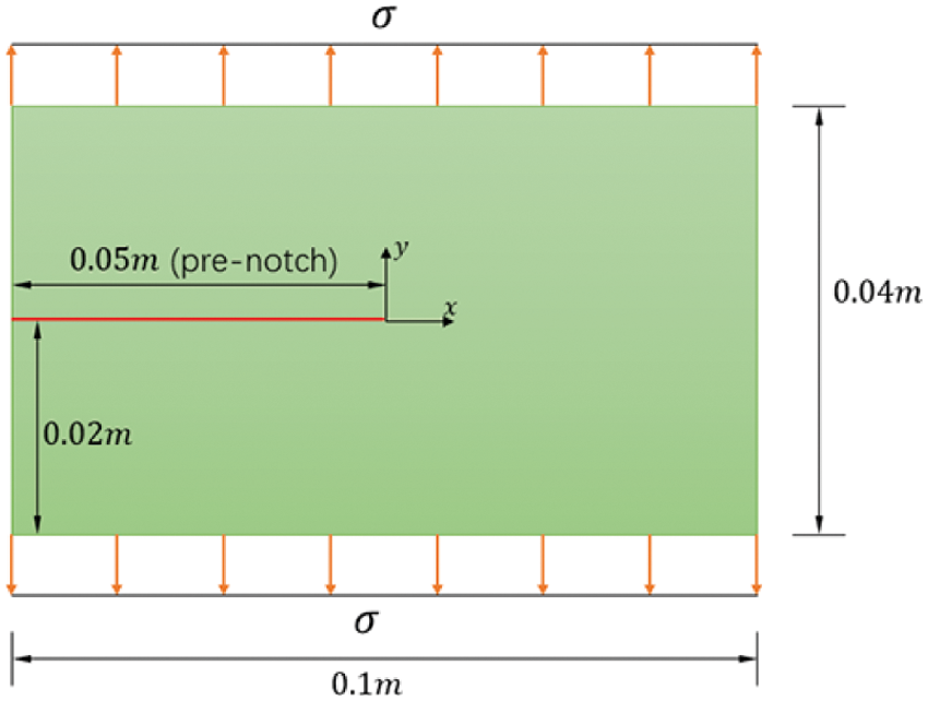
Figure 16: Initial model of thin plate with pre-notch
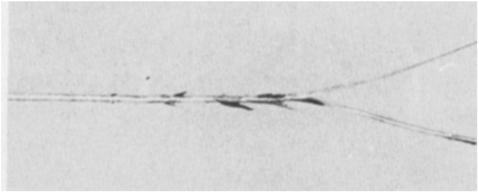
Figure 17: Crack branching in single edge notch specimen reported in experiments [44]
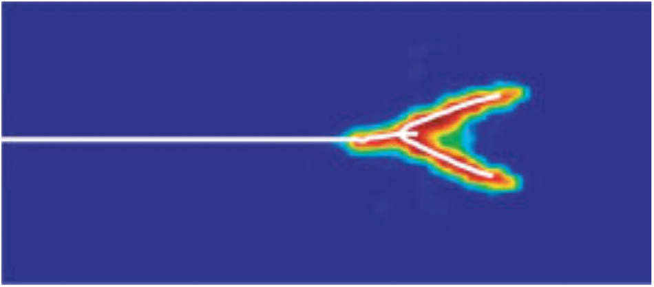
Figure 18: Crack branching in single edge notch specimen reported in experiments [43]
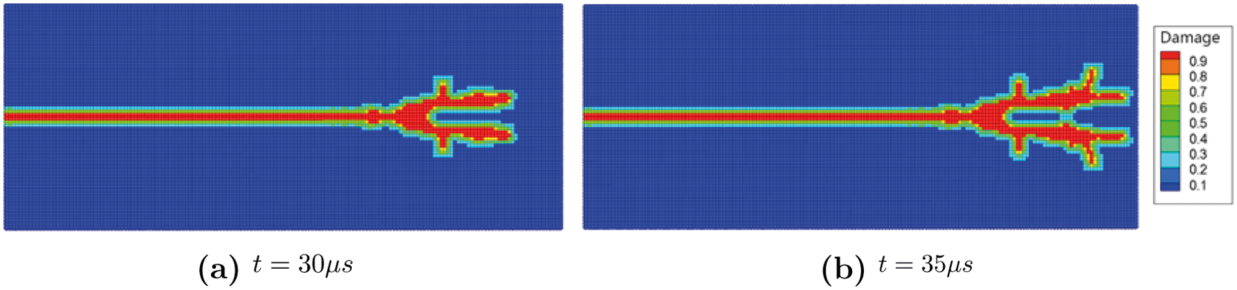
Figure 19: Crack propagation and damage distribution
3.4 Fracture Case 2: Crack Predicting and Crack Branching in Soda-Lime Glass
In this section, we use the same geometric and discretization model as in Section 3, and study the dynamic crack branching affected by the external loading with three different amplitudes. Here we use the material parameters of soda-lime glass, such that the Young’s modulus is E = 72GPa, density ρ = 2440kg/m3, and the Poisson ratio ν = 0.22. In this work, the Mohr-Coulomb failure criterion is considered. And the compressive strength and tensile strength are σc = 300Mpa and σt = 41Mpa, respectively. Step tensile loading is applied on the upper and lower boundaries of the specimen. After numerical simulation, the cracking path and the damage distribution are visualized and illustrated in Fig. 21, in which a1–c1 shows the failure state of the stress point of the plate that those failed ones are colored in red. Fig. 21 a2–c2 shows the damage contour of the material points, with the damage index ranging 0 to 1. Good consistency could be found in two representing methods in terms of the crack path and topology. One can tell that when the magnitude of loading is σ = 0.2MPa, a straight crack path is obtained, as shown in Fig. 21a, that no crack branching is observed. When the loading magnitude increases to σ = 2.0MPa, crack branching and sub-cracks are consequently generated as shown in Fig. 21b. There are several tiny crack branching that occurs before the big one, which propagates first along 45∘ and soon turns to the original cracking orientation. For larger loading magnitude σ = 4.0MPa, branching distribution has slightly changed, the big branches observed in previous loading magnitude now remain their cracking orientation after branching. Nevertheless, all the sub-cracks show high symmetry in terms of the crack propagation against the main crack. Also, the crack branching happens more intensely. Multiple branching events develop under the stress of 4.0MPa magnitude applied suddenly on the top and bottom boundaries, less branching happened later. Continued or cascading branching is the cause of fragmentation. If the energy dissipated by the formation of the first branching is overcome by the energy stored in the material, the branching process repeats, eventually leading to fragmentation.
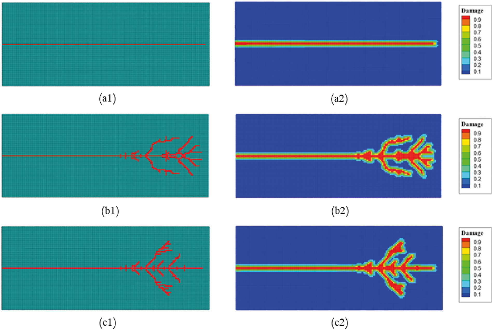
Figure 21: Damage maps in glass under suddenly applied tensile stress on boundaries with different amplitudes.a σ = 0.2MPa. b σ = 2.0MPa. c σ = 4.0MPa
The crack velocity is calculated by tracing the crack tip which is located by searching the most advanced with damage index higher than a given threshold (for current work, we choose 0.75).
We normalize velocities by the Rayleigh wave speed CVR of the material. For soda-lime glass, cVR≈3102m/s as given by [47]. Fig. 20 shows the crack propagation speeds profiles of glass under the loading amplitude σ = 2.0MPa. A vertical dash line depicts the time when the first crack branch was initialized. The crack propagation speed for the branch initiation is 0.5 times of Rayleigh wave velocity, after branching, the velocity of the cracking keeps fluctuates between 0.38 and 0.66 times of Rayleigh wave velocity. That conforms to the limiting crack speed in glass reported in experiments, which is depending on the loading conditions, and is lower than 0.66CVR [48].
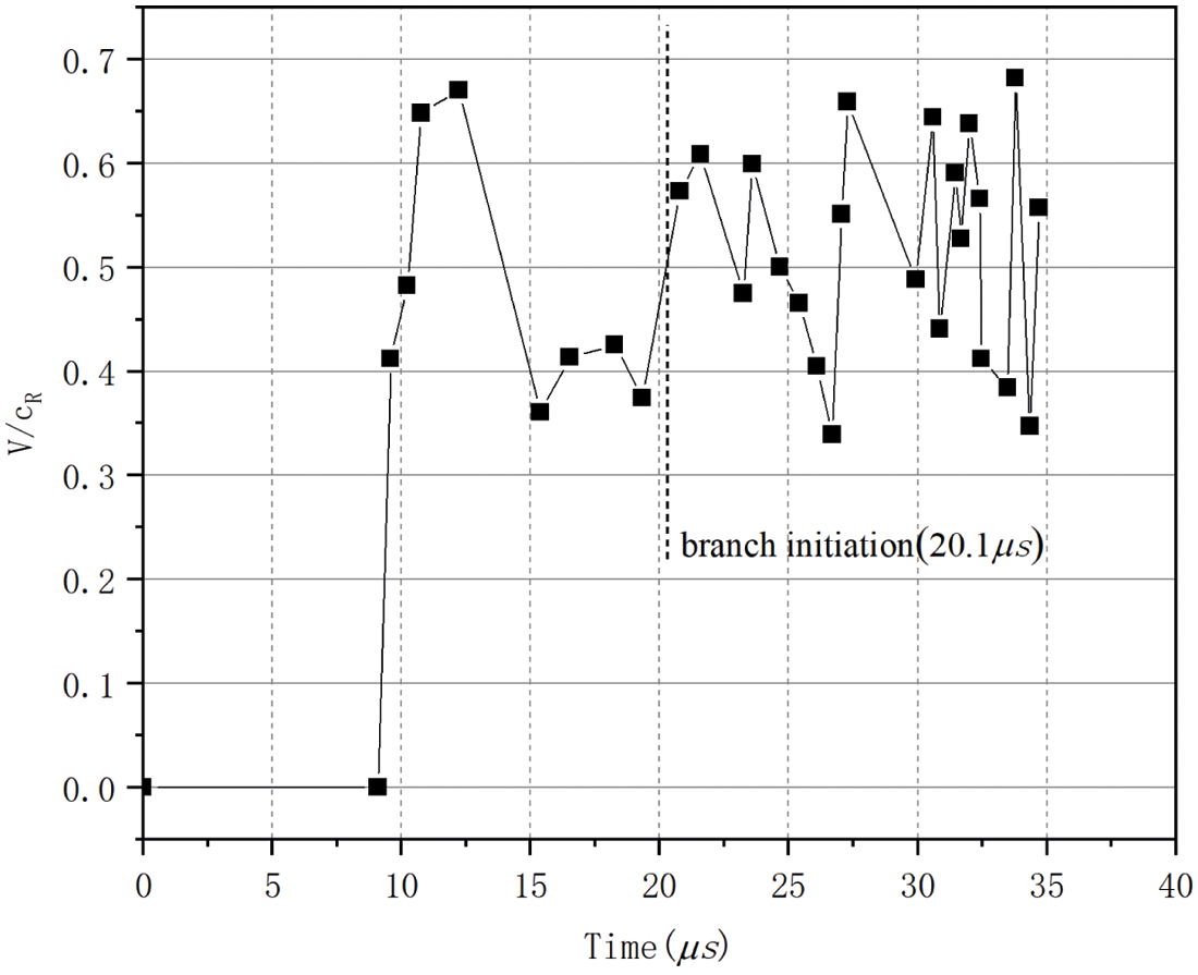
Figure 20: Crack propagation speed profiles for glass under stress boundary conditions applied on the boundaries
3.5 Fracture Case 3: A Flat Shell with a Pre-Existing Crack
A flat shell with dimensions L = 1.0 m and W = 1.0 m, and thickness h = 0.05m is investigated as shown in Fig. 22. The flat shell has a pre-existing crack at the middle with the crack length of a = 0.25m. The orientation of the initial crack is defined by angle θ as shown in Fig. 22. We investigate three cases with different initial crack orientations, which are θ = 0∘, 45∘, 90∘, respectively. The material of the flat shell has Young’s modulus of E = 32.27GPa and Poisson’s ratio ν = 0.33. The Mohr-coulomb failure criterion is used in the current work. The compressive strength and tensile strength are σc = 36MPa and σt = 2.7MPa, respectively. The left edge of the flat shell is fixed, and a linear incremental load is applied on the right edge, which is increased by Δ P = 10N/m every time step. Three fictitious layers of material points are added on the left and all degrees of freedom of these fictitious points are fixed to zero.
Fig. 23 shows the damage evolution process of the flat shell with initial crack orientation θ = 0∘. As the deflection increases, the crack propagates continuously and maintains the initial orientation until it runs through the whole shell, as shown in Fig. 23. At the beginning, the crack is placed in the center of the shell with deflection w = 0, as illustrated in Fig. 23a. As the external loading increases, the deflection becomes larger correspondingly, which initiates the cracking from both ends of the initial crack. It can be observed from the figure that, the crack propagates symmetrically in both orientations, and eventually reaches the edges of the shell, leading to the fracture of the specimen, as shown in Fig. 23d. Compare with the XFEM numerical simulation result in Fig. 24, the PD-based crack path can be better verified and in the simulation results of the two methods, when the crack penetrates, the maximum displacement of the free edge of the shell is in good agreement.
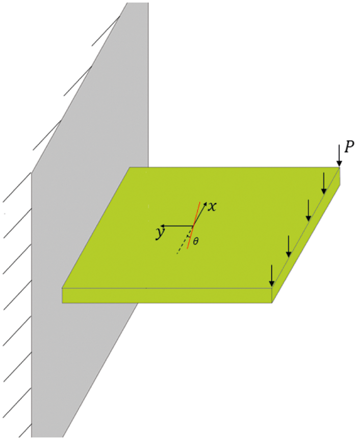
Figure 22: A flat shell with a pre-existing crack model
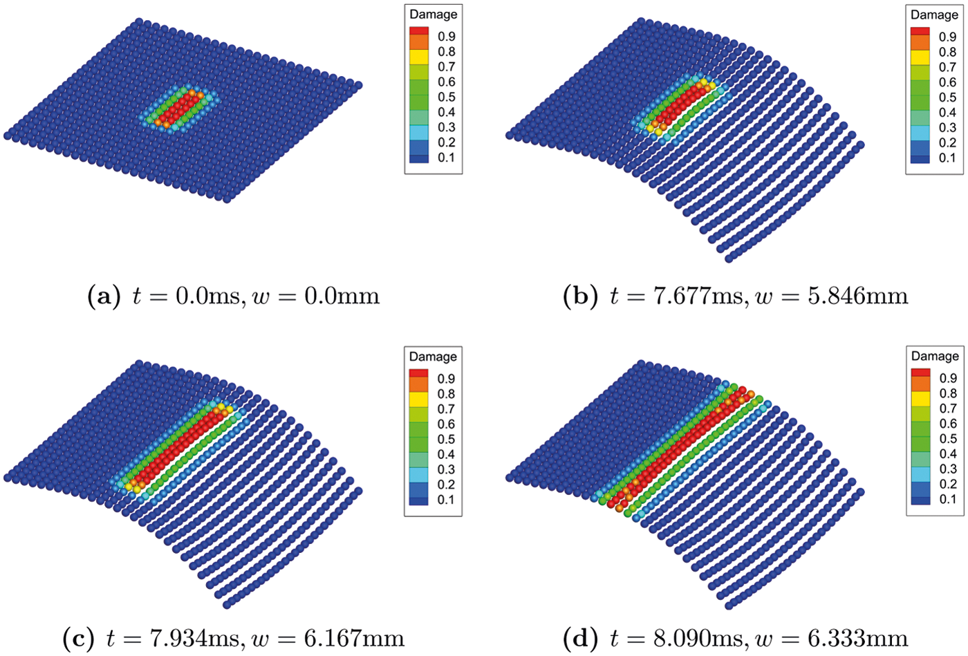
Figure 23: Contours of deflection(× 50)
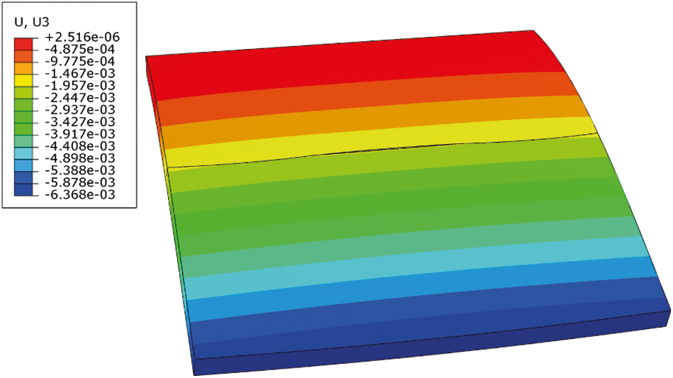
Figure 24: XFEM numerical simulation result θ = 0∘
Fig. 25 shows the damage evolution process of the flat shell with initial crack orientation θ = 45∘. The initial crack is illustrated in Fig. 25a. Figs. 25b–25d give the damage evolution process as the external loading applied increases. As the figures show, the crack starts to propagate from the very edge near the free edge of the shell where external loading is applied at time t≈30ms. As the deflection increases, the propagation goes fast from the initialization point to the one edge of the shell in a short period time, from t = 30.391ms to t = 30.512ms. It is notable that although the initial orientation of the crack is θ = 45∘, the newly propagated crack path is almost parallel to the free edge on which the external load is applied. Compare with the XFEM numerical simulation result in Fig. 26, the PD-based crack path can be better verified and in the simulation results of the two methods, when the crack penetrates, the maximum displacement of the free edge of the shell is in good agreement.
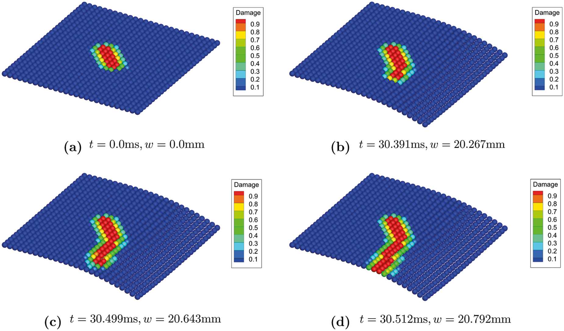
Figure 25: Contours of deflection(× 20)
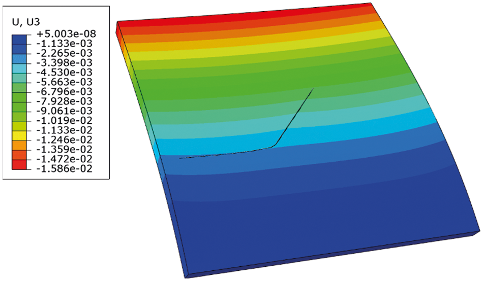
Figure 26: XFEM numerical simulation result θ = 45∘
Fig. 27 shows the damage evolution on the flat shell with initial crack orientation θ = 90∘. As the deflection increase, the crack extends towards the loading edge first as illustrated in Fig. 27b, then crack branches to two sub-cracks that are parallel to the free edge where the external load is applied. At time t = 23.986ms when the deflection w = 16.39mm, the sub-cracks runs through the shell to the both two edges, leading to the fracture, as depicted in Fig. 27d. One can also observe crack branch initiation from the very end that is near the fixed side of the shell. Compare with the XFEM numerical simulation result in Fig. 28, the PD-based crack path can be better verified.
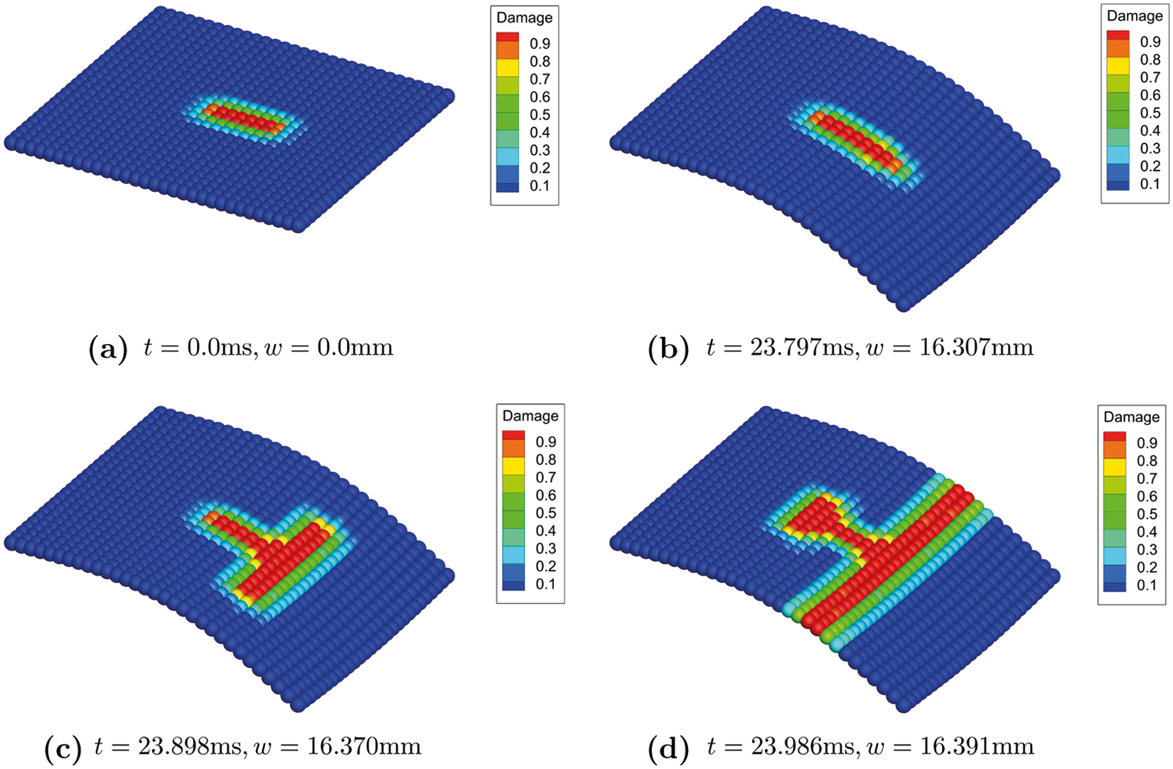
Figure 27: Contours of deflection(× 20)
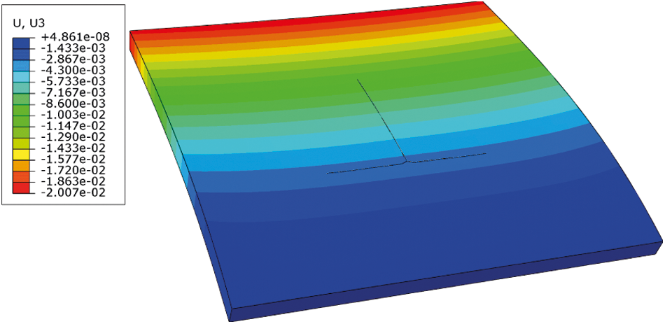
Figure 28: XFEM numerical simulation result θ = 90∘
We also analyze the damage evolution process of the flat shell with the initial crack notch at the free edge where the external loading is applied. As shown in Fig. 29, crack branching generated two sub-cracks that are perpendicular to the original crack, after which they propagate along with the orientation parallel to the loading edge of the shell. We can see in Fig. 29d, the crack propagates symmetrically in both positive and negative directions, eventually leading to the fracture of the shell as the deflection reaches w = 5.618mm. Compare with the XFEM numerical simulation result in Fig. 30, the PD-based crack path can be better verified.
Figure 29: Contours of deflection(× 20)
Figure 30: XFEM numerical simulation result
In the current work, we present a brittle fracture model of the Reissener-Mindlin shell based on the non-ordinary state-based Peridynamic shell theory. This model could be used in predicting the crack initialization and propagation. The validity of the model is validated through both quasi-static and dynamic analysis, and the accuracy and convergence of the shell model are also investigated through two numerical examples. Then, we demonstrate the capability of this model in simulating the crack growth by several numerical examples with preset crack. Comparing the simulation of current work and the experiment result and the numerical simulation result of XFEM, our model is convincing in predicting the crack path of brittle material thin shell. We believe our work provides a practical and reliable approach for thin shell brittle fracture in engineering computations. This fracture model shows the capability of the brittle fracture in terms of crack nucleation and branching for both in-plane and out-plane loads. The initiation and propagation of cracks are formed and developed naturally and spontaneously.
Acknowledgement: The authors wish to express their appreciation to the reviewers for their helpful suggestions which greatly improved the presentation of this paper.
Funding Statement: The authors would like to express grateful acknowledgement to the support from National Natural Science Foundation of China (Nos. 11802214 and 11972267) and the Fundamental Research Funds for the Central Universities (WUT: 2018IB006 and WUT: 2019IVB042).
Conflicts of Interest: The authors declare that they have no conflicts of interest to report regarding the present study.
1. Atluri, S. N., Zhu, T. (1998). A new meshless local petrov-galerkin (MLPG) approach in computational mechanics. Computational Mechanics, 22(2), 117–127. DOI 10.1007/s004660050346. [Google Scholar] [CrossRef]
2. Silling, S. (2000). Reformulation of elasticity theory for discontinuities and long-range forces. Journal of the Mechanics and Physics of Solids, 48(1), 175–209. DOI 10.1016/S0022-5096(99)00029-0. [Google Scholar] [CrossRef]
3. Foster, J. T., Silling, S. A., Chen, W. W. (2010). Viscoplasticity using peridynamics. International Journal for Numerical Methods in Engineering, 81(10), 1242–1258. DOI 10.1002/nme.2725. [Google Scholar] [CrossRef]
4. Seleson, P. (2014). Improved one-point quadrature algorithms for two-dimensional peridynamic models based on analytical calculations. Computer Methods in Applied Mechanics and Engineering, 282, 184–217. DOI 10.1016/j.cma.2014.06.016. [Google Scholar] [CrossRef]
5. Fan, H., Bergel, G. L., Li, S. (2016). A hybrid peridynamics-SPH simulation of soil fragmentation by blast loads of buried explosive. International Journal of Impact Engineering, 87, 14–27. DOI 10.1016/j.ijimpeng.2015.08.006. [Google Scholar] [CrossRef]
6. Chu, B., Liu, Q., Liu, L., Lai, X., Mei, H. (2020). A rate-dependent peridynamic model for the dynamic behavior of ceramic materials. Computer Modeling in Engineering & Sciences, 124(1), 151–178. DOI 10.32604/cmes.2020.010115. [Google Scholar] [CrossRef]
7. Chen, Z., Chu, X. (2021). Peridynamic modeling and simulation of fracture process in fiber-reinforced concrete. Computer Modeling in Engineering & Sciences, 127(1), 241–272. DOI 10.32604/cmes.2021.015120. [Google Scholar] [CrossRef]
8. Bazazzadeh, S., Zaccariotto, M., Galvanetto, U. (2019). Fatigue degradation strategies to simulate crack propagation using peridynamic based computational methods. Latin American Journal of Solids and Structures, 16(2), e163. DOI 10.1590/1679-78255022. [Google Scholar] [CrossRef]
9. Bazazzadeh, S., Morandini, M., Zaccariotto, M., Galvanetto, U. (2021). Simulation of chemo-thermo-mechanical problems in cement-based materials with peridynamics. Meccanica, 56, 2357–2379. DOI 10.1007/s11012-021-01375-7. [Google Scholar] [CrossRef]
10. Zhao, J., Lu, G., Zhang, Q., Du, W. (2021). Modelling of contact damage in brittle materials based on peridynamics. Computer Modeling in Engineering & Sciences, 129(2), 519–539. DOI 10.32604/cmes.2021.017268. [Google Scholar] [CrossRef]
11. Silling, S., Bobaru, F. (2005). Peridynamic modeling of membranes and fibers. International Journal of Non-Linear Mechanics, 40(2–3), 395–409. DOI 10.1016/j.ijnonlinmec.2004.08.004. [Google Scholar] [CrossRef]
12. O’Grady, J., Foster, J. (2014). Peridynamic plates and flat shells: A non-ordinary, state-based model. International Journal of Solids and Structures, 51(25–26), 4572–4579. DOI 10.1016/j.ijsolstr.2014.09.003. [Google Scholar] [CrossRef]
13. Diyaroglu, C., Oterkus, E., Oterkus, S., Madenci, E. (2015). Peridynamics for bending of beams and plates with transverse shear deformation. International Journal of Solids and Structures, 69–70, 152–168. DOI 10.1016/j.ijsolstr.2015.04.040. [Google Scholar] [CrossRef]
14. Chowdhury, S. R., Roy, P., Roy, D., Reddy, J. N. (2016). A peridynamic theory for linear elastic shells. International Journal of Solids and Structures, 84, 110–132. DOI 10.1016/j.ijsolstr.2016.01.019. [Google Scholar] [CrossRef]
15. Nguyen, C. T., Oterkus, S. (2019). Peridynamics for the thermomechanical behavior of shell structures. Engineering Fracture Mechanics, 219, 106623. DOI 10.1016/j.engfracmech.2019.106623. [Google Scholar] [CrossRef]
16. Hu, Y., Feng, G., Li, S., Sheng, W., Zhang, C. (2020). Numerical modelling of ductile fracture in steel plates with non-ordinary state-based peridynamics. Engineering Fracture Mechanics, 225, 106446. DOI 10.1016/j.engfracmech.2019.04.020. [Google Scholar] [CrossRef]
17. Yolum, U., Güler, M. (2020). On the peridynamic formulation for an orthotropic mindlin plate under bending. Mathematics and Mechanics of Solids, 25(2), 263–287. DOI 10.1177/1081286519873694. [Google Scholar] [CrossRef]
18. Li, S., Hao, W., Liu, W. K. (2000). Numerical simulations of large deformation of thin shell structures using meshfree methods. Computational Mechanics, 25(2–3), 102–116. DOI 10.1007/s004660050463. [Google Scholar] [CrossRef]
19. Maurel, B., Combescure, A. (2008). An SPH shell formulation for plasticity and fracture analysis in explicit dynamics. International Journal for Numerical Methods in Engineering, 76(7), 949–971. DOI 10.1002/nme.2316. [Google Scholar] [CrossRef]
20. Lin, J., Naceur, H., Coutellier, D., Laksimi, A. (2014). Geometrically nonlinear analysis of thin-walled structures using efficient shell-based SPH method. Computational Materials Science, 85, 127–133. DOI 10.1016/j.commatsci.2013.12.010. [Google Scholar] [CrossRef]
21. Peng, Y. X., Zhang, A. M., Ming, F. R. (2018). A thick shell model based on reproducing kernel particle method and its application in geometrically nonlinear analysis. Computational Mechanics, 62(3), 309–321. DOI 10.1007/s00466-017-1498-9. [Google Scholar] [CrossRef]
22. Peng, Y. X., Zhang, A. M., Ming, F. R., Wang, S. P. (2019). A meshfree framework for the numerical simulation of elasto-plasticity deformation of ship structure. Ocean Engineering, 192, 106507. DOI 10.1016/j.oceaneng.2019.106507. [Google Scholar] [CrossRef]
23. Zhang, Q., Li, S., Zhang, A. M., Peng, Y. (2021). On nonlocal geometrically exact shell theory and modeling fracture in shell structures. Computer Methods in Applied Mechanics and Engineering, 386, 114074. DOI 10.1016/j.cma.2021.114074. [Google Scholar] [CrossRef]
24. Yang, Z., Oterkus, E., Oterkus, S. (2020). A state-based peridynamic formulation for functionally graded euler-Bernoulli beams. Computer Modeling in Engineering & Sciences, 124(2), 527–544. DOI 10.32604/cmes.2020.010804. [Google Scholar] [CrossRef]
25. Shen, G., Xia, Y., Li, W., Zheng, G., Hu, P. (2021). Modeling of peridynamic beams and shells with transverse shear effect via interpolation method. Computer Methods in Applied Mechanics and Engineering, 378, 113716. DOI 10.1016/j.cma.2021.113716. [Google Scholar] [CrossRef]
26. Shen, G., Xia, Y., Hu, P., Zheng, G. (2021). Construction of peridynamic beam and shell models on the basis of the micro-beam bond obtained via interpolation method. European Journal of Mechanics-A/Solids, 86, 104174. DOI 10.1016/j.euromechsol.2020.104174. [Google Scholar] [CrossRef]
27. Silling, S. A., Epton, M., Weckner, O., Xu, J., Askari, E. (2007). Peridynamic States and Constitutive Modeling. Journal of Elasticity, 88, 151–184. DOI 10.1007/s10659-007-9125-1. [Google Scholar] [CrossRef]
28. Hughes, T. J., Liu, W. K. (1981). Nonlinear finite element analysis of shells: Part I. Three-dimensional shells. Computer Methods in Applied Mechanics and Engineering, 26(3), 331–362. DOI 10.1016/0045-7825(81)90121-3. [Google Scholar] [CrossRef]
29. Hughes, T. J., Winget, J. (1980). Finite rotation effects in numerical integration of rate constitutive equations arising in large-deformation analysis. International Journal for Numerical Methods in Engineering, 15(12), 1862–1867. DOI 10.1002/(ISSN)1097-0207. [Google Scholar] [CrossRef]
30. Zhang, Q., Li, S., Zhang, A. M., Peng, Y., Yan, J. (2020). A peridynamic Reissner-Mindlin shell theory. International Journal for Numerical Methods in Engineering, 122, 1–26. DOI 10.1002/nme.6527. [Google Scholar] [CrossRef]
31. Littlewood, D. J. (2011). A nonlocal approach to modeling crack nucleation in AA 7075-T651. in: Mechanics of solids, structures and fluids; vibration, acoustics and wave propagation, vol. 8. Denver, Colorado, USA: ASME. [Google Scholar]
32. Breitenfeld, M. S., Geubelle, P. H., Weckner, O., Silling, S. A. (2014). Non-ordinary state-based peridynamic analysis of stationary crack problems. Computer Methods in Applied Mechanics and Engineering, 272, 233–250. DOI 10.1016/j.cma.2014.01.002. [Google Scholar] [CrossRef]
33. Silling, S. A. (2016). Stability of peridynamic correspondence material models and their particle discretizations. Technical Report SAND2016–6710. [Google Scholar]
34. Li, P., Hao, Z. M., Zhen, W. Q. (2018). A stabilized non-ordinary state-based peridynamic model. Computer Methods in Applied Mechanics and Engineering, 339, 262–280. DOI 10.1016/j.cma.2018.05.002. [Google Scholar] [CrossRef]
35. Li, P., Hao, Z., Yu, S., Zhen, W. (2019). Implicit implementation of the stabilized non-ordinary state-based peridynamic model. International Journal for Numerical Methods in Engineering, 121(4), 571–587. DOI 10.1002/nme.6234. [Google Scholar] [CrossRef]
36. Chen, H. (2018). Bond-associated deformation gradients for peridynamic correspondence model. Mechanics Research Communications, 90, 34–41. DOI 10.1016/j.mechrescom.2018.04.004. [Google Scholar] [CrossRef]
37. Chen, H., Spencer, B. W. (2019). Peridynamic bond-associated correspondence model: Stability and convergence properties. International Journal for Numerical Methods in Engineering, 117(6), 713–727. DOI 10.1002/nme.5973. [Google Scholar] [CrossRef]
38. Luo, J., Sundararaghavan, V. (2018). Stress-point method for stabilizing zero-energy modes in non-ordinary state-based peridynamics. International Journal of Solids and Structures, 150, 197–207. DOI 10.1016/j.ijsolstr.2018.06.015. [Google Scholar] [CrossRef]
39. Cui, H., Li, C., Zheng, H. (2020). A higher-order stress point method for non-ordinary state-based peridynamics. Engineering Analysis with Boundary Elements, 117, 104–118. DOI 10.1016/j.enganabound.2020.03.016. [Google Scholar] [CrossRef]
40. Scordelis, A., Lo, K. (1964). Computer analysis of cylindrical shells. Journal Proceedings, 61, 539–562. DOI 10.14359/7796. [Google Scholar] [CrossRef]
41. Belytschko, T., Stolarski, H., Liu, W. K., Carpenter, N., Ong, J. S. (1985). Stress projection for membrane and shear locking in shell finite elements. Computer Methods in Applied Mechanics and Engineering, 51(1–3), 221–258. DOI 10.1016/0045-7825(85)90035-0. [Google Scholar] [CrossRef]
42. Simo, J., Fox, D., Rifai, M. (1989). On a stress resultant geometrically exact shell model. Part II: The linear theory; computational aspects. Computer Methods in Applied Mechanics and Engineering, 73(1), 53–92. DOI 10.1016/0045-7825(89)90098-4. [Google Scholar] [CrossRef]
43. Song, J. H., Areias, P. M., Belytschko, T. (2006). A method for dynamic crack and shear band propagation with phantom nodes. International Journal for Numerical Methods in Engineering, 67(6), 868–893. DOI 10.1002/(ISSN)1097-0207. [Google Scholar] [CrossRef]
44. Ramulu, M., Kobayashi, A. (1985). Mechanics of crack curving and branching-a dynamic fracture analysis. In: Williams, M. L., Knauss, W. G. (edsDynamic fracture, pp. 61–75. Dordrecht: Springer. DOI 10.1007/978-94-009-5123-5. [Google Scholar] [CrossRef]
45. Song, J. H., Wang, H., Belytschko, T. (2008). A comparative study on finite element methods for dynamic fracture. Computational Mechanics, 42(2), 239–250. DOI 10.1007/s00466-007-0210-x. [Google Scholar] [CrossRef]
46. Agwai, A., Guven, I., Madenci, E. (2011). Predicting crack propagation with peridynamics: A comparative study. International Journal of Fracture, 171(1), 65–78. DOI 10.1007/s10704-011-9628-4. [Google Scholar] [CrossRef]
47. Rahman, M., Michelitsch, T. (2006). A note on the formula for the Rayleigh wave speed. Wave Motion, 3(43), 272–276. DOI 10.1016/j.wavemoti.2005.10.002. [Google Scholar] [CrossRef]
48. Ravi-Chandar, K. (2004). Dynamic fracture. Oxford: Elsevier. [Google Scholar]
 | This work is licensed under a Creative Commons Attribution 4.0 International License, which permits unrestricted use, distribution, and reproduction in any medium, provided the original work is properly cited. |