| Computer Modeling in Engineering & Sciences |
DOI: 10.32604/cmes.2022.019097
ARTICLE
Prediction of Intrinsically Disordered Proteins Based on Deep Neural Network-ResNet18
School of Electronic Information and Optical Engineering, Nankai University, Tianjin Key Laboratory of Optoelectronic Sensor and Sensing Network Technology, Tianjin, 300350, China
*Corresponding Author: Jiaxiang Zhao. Email: zhaojx@nankai.edu.cn
Received: 02 September 2021; Accepted: 01 November 2021
Abstract: Accurately, reliably and rapidly identifying intrinsically disordered (IDPs) proteins is essential as they often play important roles in various human diseases; moreover, they are related to numerous important biological activities. However, current computational methods have yet to develop a network that is sufficiently deep to make predictions about IDPs and demonstrate an improvement in performance. During this study, we constructed a deep neural network that consisted of five identical variant models, ResNet18, combined with an MLP network, for classification. Resnet18 was applied for the first time as a deep model for predicting IDPs, which allowed the extraction of information from IDP residues in greater detail and depth, and this information was then passed through the MLP network for the final identification process. Two well-known datasets, MXD494 and R80, were used as the blind independent datasets to compare their performance with that of our method. The simulation results showed that Matthew’s correlation coefficient obtained using our deep network model was 0.517 on the blind R80 dataset and 0.450 on the MXD494 dataset; thus, our method outperformed existing methods.
Keywords: ResNet18; MLP; intrinsically disordered protein
Intrinsically disordered proteins (IDPs) (i.e., proteins that contain disordered regions [1,2]) have been confirmed to be related to many important biological activities and involved in several important cell functions, such as nucleic acid folding [3] and cell signaling and regulation [4,5]. Moreover, various human diseases, such as certain types of cancers [6], genetic diseases, and Alzheimer’s disease [7,8] are associated with IDPs. Furthermore, IDPs are more easily blocked by small molecules, and are therefore potential targets for drug design, providing a good basis for drug treatment [9,10]. However, accurately, reliably, and rapidly identifying IDPs remains a challenging problem.
Numerous schemes for detecting IDPs have been proffered over the past several decades and can be categorized into two types: those based on physical and chemical properties of amino acids and those based on computational methods. (i) examples based on physicochemical properties include FoldIndex [11], GlobPlot [12], FoldUnfold [13], and IsUnstruct [14]. FoldIndex [11] predicts disordered proteins by calculating the ratio of the average hydrophobicity to the average net charge of the residues. GlobPlot [12] predicts the disordered region by analyzing the tendency of all amino acids in the protein sequence to disordered residues and ordered residues. FoldUnfold [13] treats areas with a weaker density as unnecessary areas by predicting the average packing density of residues. IsUnstruct [14] is a prediction method based on statistical physics and uses the Ising model for disorder-order transformations in protein sequences and replaces the interactions of adjacent terms with penalties for changes between boundary energy states. These methods promote the field of IDPs, yet ignore the overall structure of the protein, which leads to inaccurate prediction results. (ii) More recently, the use of machine learning has increased in the field of bioinformatics, especially to solve problems that are closely related to human life and health [15,16]. Methods to identify IDPs through machine learning, especially deep learning techniques, such as PONDR [17], DISOPRED2 [18], RONN [19], DISKNN [20], IDP-Seq2Seq [21], NetSurfP-2.0 [22], SPOT-Disorder2 [23], and RFPR-IDP [24], have also been developed. The PONDR [17] series is the first publicly available and established method for predicting IDPs internationally, which distinguishes disordered proteins from ordered proteins based primarily on differences in their amino acid composition. DISOPRED2 [18] is a dynamic prediction method for disordered proteins, and the output of the support vector machine is used as the prediction results. RONN [19] is a function-based array and neural network prediction algorithm. Its main idea is that if two proteins have similar biological functions and similar tendencies toward being disordered or ordered, then their sequences are also similar. DISKNN [20] applies KNN with several protein features to predict the disordered regions of proteins. However, the performance comparison in this article was unconvincing because it was only regarding one protein. IDP-Seq2Seq [21] draws on sequence-to-sequence learning in natural language processing to map protein sequences and use associations between residues as features for prediction. NetSurfP-2.0 [22] applies convergence strategies with the convolutional neural network (CNN) and long and short-term memory networks (LSTM) based on protein structural features. SPOT-Disorder2 [23] is an improvement of the SPOT-Disorder by Hanson et al. [25] (a profile-based method), which mainly uses the LSTM model to predict intrinsically disordered proteins. RFPR-IDP [24] is based on a combination of the CNN and the bidirectional LSTM. In addition, there are also various meta-methods to predict IDPs, such as IDP-FSP [26], MFDp [27], Spark-IDPP [28], and Meta-Disorder [29], which run multiple independent prediction schemes and merge their results to obtain final prediction results. Mishra et al. used a deep learning-integrated method combining 9890 features for protein function prediction; the large number of features used was novel [30]. These schemes based on computational methods do not sufficiently capture details between protein residues and only capture those at the sequence level, which leads to inaccurate predictions.
Thus, in the field of predicting IDPs, several problems remain: (i) Predictions using physical and chemical methods is not only a complex and time-consuming process but also have poor prediction performance; (ii) Previous studies based on computational methods did not employ a sufficiently deep network to capture more accurate characteristics among residues, and consequently, did not demonstrate a significant improvement in performance; (iii) Although some previous methods have advantages in predicting IDPs, Matthew's correlation coefficient (MCC) [31], which directly indicates the quality of the prediction result, remain relatively low on blind independent test datasets.
Motivation: Because IDPs are essential given their important roles in various human diseases and their association with many important biological activities, addressing the above three problems in an accurate, reliable, and rapid manner is of great significance and research value. Therefore, using simple computational methods, rather than complex physicochemical methods, is crucial, and constructing a neural network with deep layers for predicting IDPs and demonstrating an improvement in prediction performance is essential. ResNet18 [32] has sufficiently deep layers and has been used in myriad domains owing to its excellent performance; however, it is the first application of ResNet18 for predicting IDPs. It would be constructive to apply the ResNet18 deep neural network and achieve good results, with a high as possible MCC value, for predicting IDPs.
Contribution: During this study, we proposed a novel method for predicting IDPs using deep neural networks, which outperformed existing methods. The innovative value of our contributions are as follows:
• We constructed a sufficiently deep structure, which consisted of five identical ResNet18 networks, and combined it with a constructed multilayer perceptron (MLP) network. This constructure differed from all previous methods and was a completely new architecture. Fig. 1 depicts the paradigm of our deep neural structure.
• Resnet18 was applied for the first time as a deep network model for predicting IDPs. The study did not simply use the ResNet18 network directly but replaced the output layer with a dense layer, and the output was then input into the MLP network.
• The simulation results showed that the MCC value obtained using our deep network model was a significant improvement on other existing methods, which has important implications for more precise investigations of IDPs.
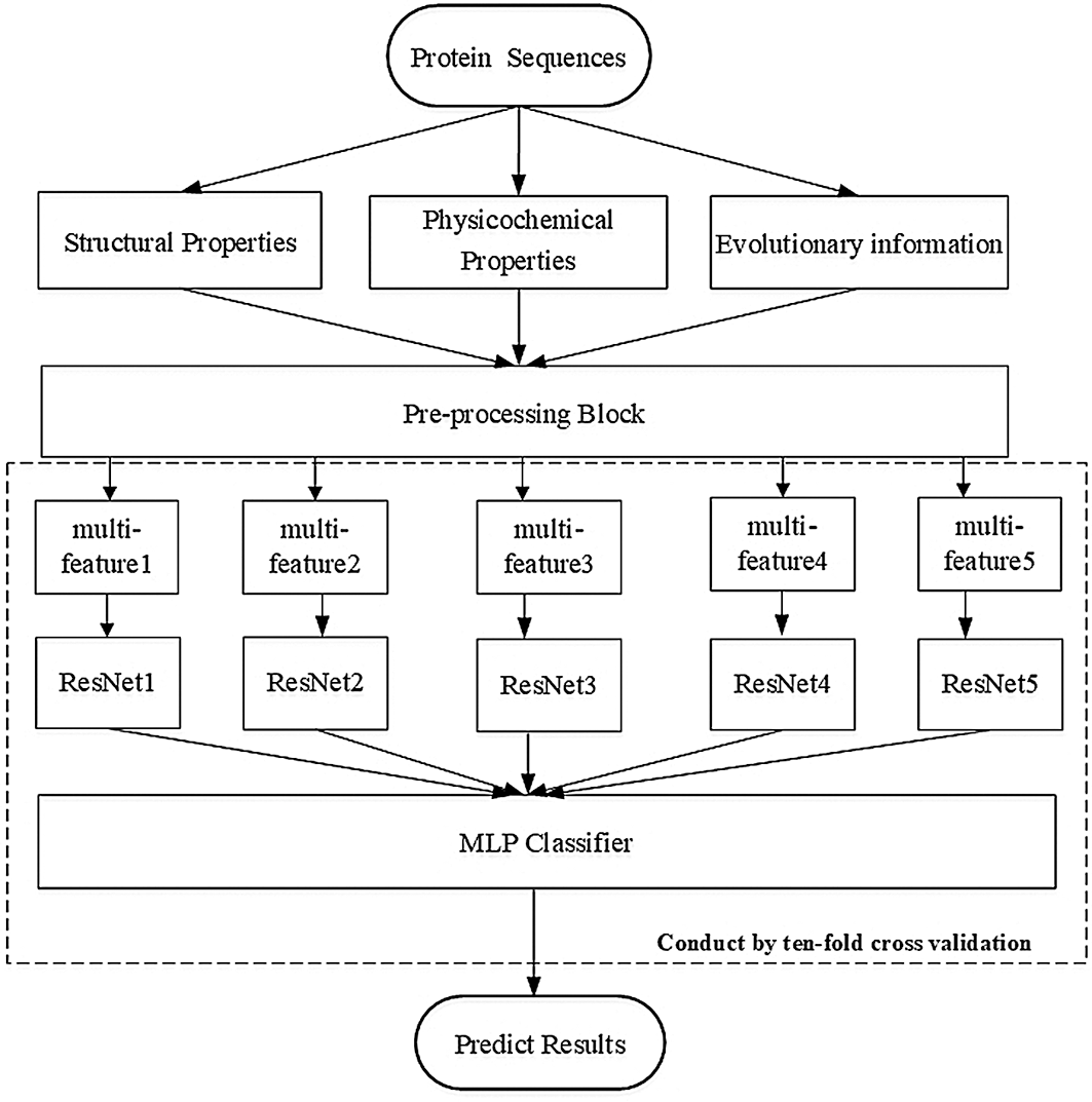
Figure 1: Paradigm of our deep neural structure
The following steps illustrate the specific performing process of our proposed method in detail:
Step 1. Data preparation: A total of 1616 pieces of the latest protein sequences were downloaded from the DisProt database as a training dataset for our deep network model.
Step 2. Feature selection: For the features of each amino acid of the IDP sequence, we calculated five structural properties, seven physicochemical properties, and 20 protein evolution information of the sequence with a total of 32 features; the five structural properties included Shannon entropy [33], topological entropy [33,34], and three amino-acid propensity scales; the seven physicochemical properties were obtained from Meiler et al. [35], and the position-specific scoring matrices (PSSMs) were generated from the PSI-BLAST software using the latest NCBI non-redundant database [36] (updated in June 2020).
Step 3. Feature pre-processing: An important step after selecting features is preprocessing features using the sliding window approach. With the sliding calculation of the window over each protein sequence, we obtained the feature matrix
Step 4. Model processing: We constructed a sufficiently deep structure, which consisted of five identical ResNet18 networks, and combined it with a constructed MLP network. For the original ResNet18 model, we replaced the fully connected (FC) layer with a dense layer, and the output was then input into the MLP network for the final identification process.
Step 5. Analyze the blind dataset performance: In contrast to other well-known methods, the R80 and MXD494 datasets were used as our blind datasets to analyze the performance of our deep network model.
The different sections of this article describe the contents of the proposed method in a step-by-step manner and are organized according to the above steps as follows: Section 2 describes above Steps 1 to 4 and the materials and methods proposed in this article, which include the preparation of our method, the architecture of the network, and how the method works. Section 3 compares other well-known methods that predict IDPs using five recognized performance measures. Section 4 provides our conclusions and the future scope of our research.
We have listed all datasets used for training and blind testing, and we introduce the architecture of our deep network model depicted in Fig. 1. The model is comprised of a pre-processing block, five copies of the ResNet18, and a self-constructed MLP network.
We employed DIS1616 from the latest version of the DisProt database as our training dataset. The DIS1616 dataset consists of 1616 protein sequences, which comprise 888678 residues. Of these 888678 residues, 182316 are disordered residues and 706362 are ordered residues. Here, we randomly shuffled and divided the dataset into 10 separate subsets, with the test dataset containing 166 sequences. Then, 10-fold cross-validation was performed. To analyze the performance of our deep network, the R80 [19] and MXD494 datasets [21,37] were used as our blind datasets. The R80 dataset consisted of 80 protein sequences with 3566 disordered residues and 29243 ordered residues. The MXD494 dataset contained 494 protein sequences with 44087 disordered residues and 152474 ordered residues. Fig. 2 illustrates two completely ordered proteins (2FG1 and 3BBB) with stable three-dimensional structures from the MXD494 dataset.
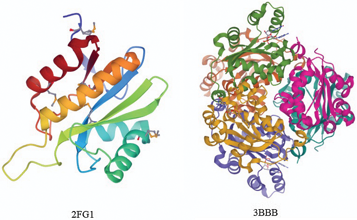
Figure 2: Two protein pictures from the MXD494 dataset
2.2 Protein Feature Selection and Pre-Processing Procedure
Three types of features were selected: five features associated with the structural properties, seven features corresponding to the physicochemical properties, and the remaining features related to the evolutionary information. Structural features were Shannon entropy [33], topological entropy [33,34], and three amino acid propensity scales provided in the GlobPlot NAR paper [12]. The physicochemical features were obtained from Meiler et al. [35]. The PSSMs were used to describe the protein evolution information generated from the PSI-BLAST software using the latest NCBI non-redundant database [36] (updated in June 2020).
As shown in Fig. 1, our deep neural network contained a pre-processing block that computed the input feature matrix
1) For each residue in a given protein sequence of length L, a window of size M centered around this residue was chosen. We added
where
where
2) For the i-th residue (
where
Fig. 1 shows that the output of the pre-processing block yielded the feature matrix in Eq. (3) of the i-th (
2.3 Designing and Training the ResNet18 and MLP Models
We constructed a sufficiently deep structure, which consisted of five variant ResNet18 networks, and combined it with a constructed MLP network. Fig. 3 shows each of the five identical variant deep neural structures that replaced the FC layer with a dense layer containing 16 perceptrons. The outputs of the five variant networks were then concatenated and input into the MLP network that we constructed for the prediction.
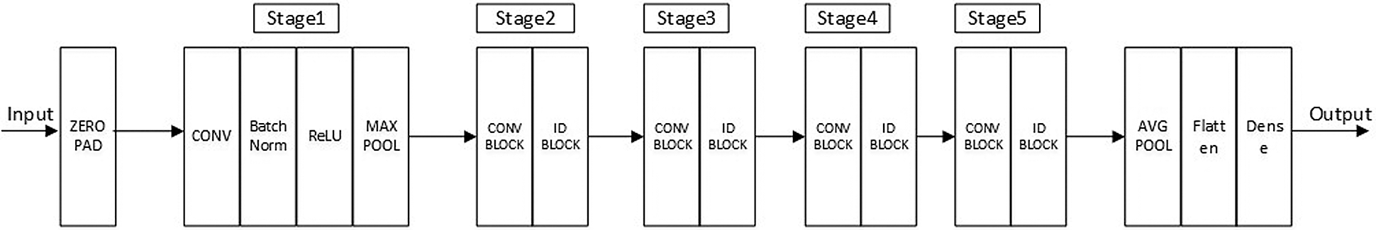
Figure 3: Frame diagram of the variant ResNet18 model
The MLP network we constructed had two hidden layers, where the binary cross-entropy cost function was employed:
In Eq. (4),
The output of each of our variant ResNet18 models in Fig. 1 was a
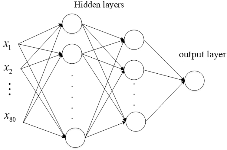
Figure 4: Structure of the MLP network
We randomly initialized the parameters of the MLP model and employed an stochastic gradient descent (SGD) optimizer to perform back-propagation to update the parameters during the training process. The output of the sigmoid function was thus used as the predicted probability
where
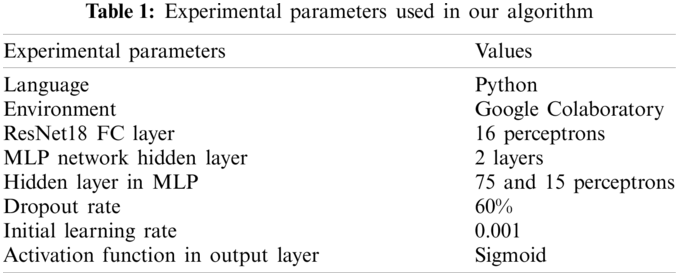
The training process with our constructed model was as follows: first, we randomly shuffled and split the training dataset into multiple batches and calculated the probabilities of all residues in each batch through the constructed network using Eq. (5). Subsequently, the binary cross-entropy loss function was employed to compute the loss of the given batch, to optimize the network parameters through the SGD optimization mechanism for the back-propagation process, where the learning rate was set to 0.001. The above procedure was repeated for every batch of residues until one epoch was completed (i.e., all residues were trained by the network, and probabilities were calculated). After one epoch was completed, we then randomly shuffled and split the training dataset into multiple batches again and repeated the whole procedure until the loss stopped converging or the training epoch reached the setting number. The main parameters of our algorithm are summarized in Table 1.
After the training process was complete and our network parameters were determined, we used the test dataset to test our network. The predicted probabilities obtained using Eq. (5) were used to determine whether the residue was disordered or ordered. Finally, we conducted the performance evaluation.
To evaluate the accuracy of our model for predicting IDPs, we mainly used five authoritative and universal evaluation criteria in the IDP prediction field: sensitivity (Sen), specificity (Spe), binary accuracy (BAcc), weight score (Sw), and MCC. TP, FP, TN, and FN were also used to respectively denote the numbers of true disordered, false disordered, true ordered, and false ordered samples. The following formulae were used to calculate these five evaluation criteria:
Among these, the MCC value was the most important and effective criterion to measure the performance of the prediction of IDPs, which varies from −1 to 1. A high MCC value indicates outstanding classification performance.
3.1 Comparison of Performance with Other Well-known Methods
For ease of description, DISRES was employed as the acronym of our deep network model. To analyze the performance of our deep network model and highlight the advantages of our method, DISRES was compared with seven other state-of-the-art methods used for predicting IDPs, using the five performance measures described above using two blind datasets: MXD494 and R80. The MCC value obtained by our trained model was 0.450 for the blind MXD494 dataset and 0.517 for the R80 dataset. Therefore, the MCC values obtained using our network model showed that our model outperformed the existing methods of DISpre, SPOT-Disorder2, RFPR-IDP, DISOPRED2, DISpro, RONN, PONDR, and FoldIndex. All relevant evaluation criteria for comparing the performance of the models using the two blind datasets, MXD494 and R80, are shown in Tables 2 and 3. To visualize the comparison results, Figs. 5 and 6 show the comparisons of performance between different methods using the two blind datasets, respectively, where the red line represents MCC, the most important evaluation criteria, for prediction performance.
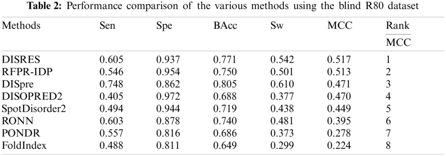
As shown in Table 2, for the blind R80 test dataset, DISRES showed superiority over the other seven well-known methods for predicting IDPs, with an MCC value of 0.517, and ranking first among all methods. DISpre is a method we developed previously in relation to MCC using the MLP network alone. Fig. 5 shows that DISpre achieved the highest sensitivity value but obtained lower specificity and MCC value, which resulted in poor predictive performance. The MCC value significantly improved with the addition of the ResNet18 deep neural network, and the value obtained by DISRES was on the highest point of the red line, which demonstrated that our method yielded the best performance in predicting IDPs.
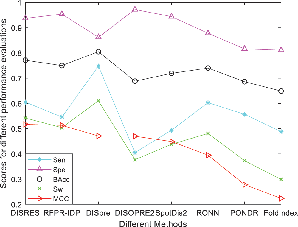
Figure 5: Comparisons of the different methods using the blind R80 dataset
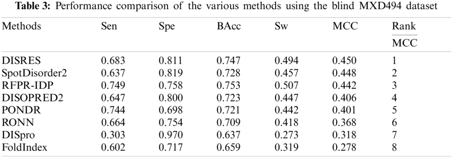
To make the results more convincing, we used another widely used blind test dataset, the MXD494, which contains more data than R80. As shown in Table 3, DISRES achieved an MCC of 0.450, which was higher than that of several other prediction methods; moreover, it still ranked first among all methods, which can largely be attributed to the deep neural network ResNet18 applied in DISRES. Although the PONDR obtained the best specificity, as shown in Fig. 6, its sensitivity and MCC value were low, which indicated that the PONDR did not perform well in predicting IDPs. DISRES still achieved the highest point on the red line of MCC, which showed that it outperformed the other methods.
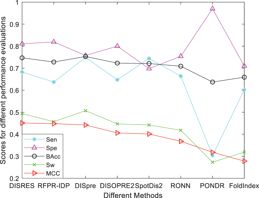
Figure 6: Comparisons of the different methods using the blind MXD494 dataset
3.2 Limitations of the Current Study
For the first time, we used the deep neural network model, ResNet18, and combined it with an MLP network to predict disordered regions of IDPs with good performance. However, it is well known that the size of the training dataset in a neural network affects the final prediction results. Although the dataset we obtained from the authoritative DisProt database is the most recent data available, there were still only 1616 protein sequences, which limits the potential of improving the performance of our model.
IDPs are of great importance as they play essential roles in numerous human diseases, such as certain types of cancers, genetic diseases, and Alzheimer’s disease; moreover, they are related to many important biological activities, such as nucleic acid folding and cell signaling and regulation. Thus, developing a method that can accurately, reliably, and rapidly identify IDPs is important to understand the mechanisms underlying biological activities and study the role of IDPs in major diseases. Therefore, our proposed method for efficiently detecting IDPs has important practical implications for research on biological activities.
In contrast to other previously proposed methods, our model has the following advantages: (i) fewer features were selected to achieve better results than other methods; (ii) a sufficiently deep neural network, ResNet18, was introduced for the prediction and achieved the most accurate predictions; (iii) most convincingly, the MCC values obtained using our method were the highest.
The outperforming of our constructed model over other methods was mainly attributed to the following points: (i) the construction of a sufficiently deep structure, which consisted of five identical ResNet18 networks, and its combination with a constructed MLP network. This constructure differed from all previous methods and was a completely new architecture; (ii) Resnet18 was applied for the first time as a deep network model for predicting IDPs, which enabled the extraction of information from IDP residues in greater detail and depth than those of other methods; (iii) using two well-known datasets, MXD494 and R80, as blind test datasets, simulation results showed that the MCC values obtained using our method were 0.517 for the blind R80 dataset and 0.450 from the MXD494 dataset, which demonstrated that our method outperformed existing methods.
In the future, we will approach subsequent research from two perspectives: (i) the extraction of protein features; exploring additional properties of amino acids may improve prediction performance; (ii) models developed based on other deep learning methods to further improve prediction performance.
Funding Statement: The authors received no specific funding for this study.
Conflicts of Interest: The authors declare that they have no conflicts of interest to report regarding the present study.
1. Deng, X., Eickholt, J., Cheng, J. (2011). A comprehensive overview of computational protein disorder prediction methods. Molecular Biosystems, 8(1), 114–121. DOI 10.1039/C1MB05207A. [Google Scholar] [CrossRef]
2. Liu, Y., Wang, X., Liu, B. (2017). A comprehensive review and comparison of existing computational methods for intrinsically disordered protein and region prediction. Briefings in Bioinformatics, (1), 330–346. DOI 10.1093/bib/bbx126. [Google Scholar] [CrossRef]
3. Holmstrom, E. D., Liu, Z., Nettels, D., Best, R. B., Schule, B. (2019). Disordered RNA chaperones can enhance nucleic acid folding via local charge screening. Nature Communications, 10(1), 2453. DOI 10.1038/s41467-019-10356-0. [Google Scholar] [CrossRef]
4. Wright, P. E., Dyson, H. J. (2015). Intrinsically disordered proteins in cellular signaling and regulation. Nature Reviews Molecular Cell Biology, 16(1), 18–29. DOI 10.1038/nrm3920. [Google Scholar] [CrossRef]
5. Iakoucheva, L. M., Brown, C. J., Lawson, J. D., Obradovi, Z., Dunker, A. K. (2002). Intrinsic disorder in cell-signaling and cancer-associated proteins. Journal of Molecular Biology, 323(3), 573–584. DOI 10.1016/S0022-2836(02)00969-5. [Google Scholar] [CrossRef]
6. Kulkarni, V., Kulkarni, P. (2019). Intrinsically disordered proteins and phenotypic switching: Implications in cancer. Progress in Molecular Biology and Translational Science, 166(1), 63–84. DOI 10.1016/bs.pmbts.2019.03.013. [Google Scholar] [CrossRef]
7. Pankratz, N., Nichols, W. C., Elsaesser, V. E., Pauciulo, M. W., Foroud, T. (2010). Alpha-synuclein and familial Parkinson’s disease. Movement Disorders, 24(8), 1125–1131. DOI 10.1002/mds.22524. [Google Scholar] [CrossRef]
8. Uversky, V. N., Oldfield, C. J., Midic, U., Xie, H., Xue, B. et al. (2009). Unfoldomics of human diseases: Linking protein intrinsic disorder with diseases. BMC Genomics, 10(1), 1–17. DOI 10.1186/1471-2164-10-S1-S7. [Google Scholar] [CrossRef]
9. Uversky, V. N. (2014). Introduction to intrinsically disordered proteins (IDPS). Chemical Reviews, 114(13), 6557–6560. DOI 10.1021/cr500288y. [Google Scholar] [CrossRef]
10. He, H., Zhao, J., Sun, G. (2019). The prediction of intrinsically disordered proteins based on feature selection. Algorithms, 12(2), 46. DOI 10.3390/a12020046. [Google Scholar] [CrossRef]
11. Prilusky, J., Felder, C. E., Zeev-Ben-Mordehai, T., Rydberg, E. H., Sussman, J. L. (2005). FoldIndex: A simple tool to predict whether a given protein sequence is intrinsically unfolded. Bioinformatics, 21(16), 3435–3438. DOI 10.1093/bioinformatics/bti537. [Google Scholar] [CrossRef]
12. Rune, L., Russell, R. B., Victor, N., Gibson, T. J. (2003). Globplot: Exploring protein sequences for globularity and disorder. Nucleic Acids Research, 31(13), 3701–3708. DOI 10.1093/nar/gkg519. [Google Scholar] [CrossRef]
13. Galzitskaya, O. V., Lobanov, G. M. Y. (2006). Foldunfold: Web server for the prediction of disordered regions in protein chain. Bioinformatics, 22(23), 2948–2949. DOI 10.1093/bioinformatics/btl504. [Google Scholar] [CrossRef]
14. Lobanov, M. Y., Galzitskaya, O. V. (2011). The Ising model for prediction of disordered residues from protein sequence alone. Physical Biology, 8(3), 035004. DOI 10.1088/1478-3975/8/3/035004. [Google Scholar] [CrossRef]
15. Alyasseri, Z. A., Al-Betar, M. A., Doush, I. A., Awadallah, M. A., Abasi, A. K. et al. (2021). Review on COVID-19 diagnosis models based on machine learning and deep learning approaches. Expert Systems, 80(1), 1. DOI 10.1111/exsy.12759. [Google Scholar] [CrossRef]
16. Lakhan, A., Mohammed, M. A., Kozlov, S., Rodrigues, J. J. P. C. (2021). Mobile-fog-cloud assisted deep reinforcement learning and blockchain-enable IoMT system for healthcare workflows. Transactions on Emerging Telecommunications Technologies, 19(2), 1. DOI 10.1002/ett.4363. [Google Scholar] [CrossRef]
17. Peng, K., Vucetic, S., Radivojac, P., Brown, C. J., Dunker, A. K. et al. (2011). Optimizing long intrinsic disorder predictors with protein evolutionary information. Journal of Bioinformatics and Computational Biology, 3(1), 35–60. DOI 10.1142/S0219720005000886. [Google Scholar] [CrossRef]
18. Ward, J. J., Sodhi, J. S., McGuffin, L. J., Buxton, B. F., Jones, D. T. (2004). Prediction and functional analysis of native disorder in proteins from the three kingdoms of life. Journal of Molecular Biology, 337(3), 635–645. DOI 10.1016/j.jmb.2004.02.002. [Google Scholar] [CrossRef]
19. Yang, Z. R., Thomson, R., McNeil, P., Esnouf, R. M. (2005). RONN: The bio-basis function neural network technique applied to the detection of natively disordered regions in proteins. Bioinformatics, 21(16), 3369–3376. DOI 10.1093/bioinformatics/bti534. [Google Scholar] [CrossRef]
20. Yang, J., Liu, H., He, H. (2020). Prediction of intrinsically disordered proteins with a low computational complexity method. Computer Modeling in Engineering & Sciences, 125(1), 111–123. DOI 10.32604/cmes.2020.010347. [Google Scholar] [CrossRef]
21. Tang, Y. J., Pang, Y. H., Liu, B. (2020). Idp-seq2seq: Identification of intrinsically disordered regions based on sequence-to-sequence learning. Bioinformatics, 17(21), 396–404. DOI 10.1093/bioinformatics/btaa667. [Google Scholar] [CrossRef]
22. Klausen, M. S., Jespersen, M. C., Nielsen, H. (2019). NetSurfP-2.0: Improved prediction of protein structural features by integrated deep learning. Proteins: Structure, Function, and Bioinformatics, 87(6), 520–527. DOI 10.1002/prot.25674. [Google Scholar] [CrossRef]
23. Hanson, J., Paliwal, K. K., Litfin, T., Zhou, Y. (2019). Spot-disorder2: Improved protein intrinsic disorder prediction by ensembled deep learning. Genomics, Proteomics and Bioinformatics, 17(6), 645–656. DOI 10.1016/j.gpb.2019.01.004. [Google Scholar] [CrossRef]
24. Liu, Y., Wang, X., Liu, B. (2020). RFPR-IDP: Reduce the false positive rates for intrinsically disordered protein and region prediction by incorporating both fully ordered proteins and disordered proteins. Briefings in Bioinformatics, 22(2), 2000–2011. DOI 10.1093/bib/bbaa018. [Google Scholar] [CrossRef]
25. Hanson, J., Yang, Y., Paliwal, K., Zhou, Y. (2017). Improving protein disorder prediction by deep bidirectional long short-term memory recurrent neural networks. Bioinformatics, 33(5), 685–692. DOI 10.1093/bioinformatics/btw678. [Google Scholar] [CrossRef]
26. Liu, Y., Chen, S., Wang, X., Liu, B. (2019). IDP-FSP: Identification of intrinsically disordered proteins/regions by length-dependent predictors based on conditional random fields. Molecular Therapy-Nucleic Acids, 17(D1), 396–404. DOI 10.1016/j.omtn.2019.06.004. [Google Scholar] [CrossRef]
27. Mizianty, M. J., Stach, W., Chen, K., Kedarisetti, K. D., Disfani, F. M. et al. (2010). Improved sequence-based prediction of disordered regions with multilayer fusion of multiple information sources. Bioinformatics, 26(18), i489–i496. DOI 10.1093/bioinformatics/btq373. [Google Scholar] [CrossRef]
28. Maysiak-Mrozek, B., Baron, T., Mrozek, D. (2019). Spark-IDPP: High-throughput and scalable prediction of intrinsically disordered protein regions with spark clusters on the cloud. Cluster Computing, 22(17), 487–508. DOI 10.1007/s10586-018-2857-9. [Google Scholar] [CrossRef]
29. Kozlowski, L. P., Bujnicki, J. M. (2012). Meta-disorder: A meta-server for the prediction of intrinsic disorder in proteins. BMC Bioinformatics, 13(1), 111. DOI 10.1186/1471-2105-13-111. [Google Scholar] [CrossRef]
30. Mishra, S., Rastogi, Y. P., Jabin, S. (2019). A deep learning ensemble for function prediction of hypothetical proteins from pathogenic bacterial species. Computational Biology and Chemistry, 83(3), 107–147. DOI 10.1016/j.compbiolchem.2019.107147. [Google Scholar] [CrossRef]
31. Liu, B., Xu, J., Fan, S., Xu, R., Zhou, J. et al. (2015). PSEDNA-PRO: DNA-binding protein identification by combining Chou’s PseAAC and physicochemical distance transformation. Molecular Informatics, 34(1), 8–17. DOI 10.1002/minf.201400025. [Google Scholar] [CrossRef]
32. He, K., Zhang, X., Ren, S., Sun, J. (2016). Deep residual learning for image recognition. IEEE Conference on Computer Vision and Pattern Recognition, pp. 770–778. Las Vegas, USA. [Google Scholar]
33. He, H., Zhao, J. (2018). A low computational complexity scheme for the prediction of intrinsically disordered protein regions. Mathematical Problems in Engineering, 2018, 1–7. DOI 10.1155/2018/8087391. [Google Scholar] [CrossRef]
34. Jin, S., Tan, R., Jiang, Q., Li, X., Peng, J. et al. (2014). A generalized topological entropy for analyzing the complexity of DNA sequences. PLoS One, 9(2), e88519. DOI 10.1371/journal.pone.0088519. [Google Scholar] [CrossRef]
35. Meiler, J., Müller, M., Zeidler, A., Schmäschke, F. (2001). Generation and evaluation of dimension-reduced amino acid parameter representations by artificial neural networks. Journal of Molecular Modeling, 7(9), 360–369. DOI 10.1007/s008940100038. [Google Scholar] [CrossRef]
36. Pruitt, K. D., Tatiana, T., William, K., Maglott, D. R. (2009). NCBI reference sequences: Current status, policy and new initiatives. Nucleic Acids Research, 37, D32–36. DOI 10.1093/nar/gkn721. [Google Scholar] [CrossRef]
37. Peng, Z. L., Kurgan, L. (2012). Comprehensive comparative assessment of in-silico predictors of disordered regions. Current Protein & Peptide Science, 13(1), 6–18. DOI 10.2174/138920312799277938. [Google Scholar] [CrossRef]
 | This work is licensed under a Creative Commons Attribution 4.0 International License, which permits unrestricted use, distribution, and reproduction in any medium, provided the original work is properly cited. |