| Computer Modeling in Engineering & Sciences |
DOI: 10.32604/cmes.2022.019221
ARTICLE
Modeling the Spread of Tuberculosis with Piecewise Differential Operators
1Institute for Groundwater Studies, Faculty of Natural and Agricultural Sciences, University of the Free State, Bloemfontein, 9301, South Africa
2Department of Medical Research, China Medical University Hospital, China Medical University, Taichung, 008864, Taiwan
3Department of Accounting and Financial Management, Seydikemer High School of Applied Sciences, Mugla Sitki Kocman University, Mugla, 48300, Turkey
*Corresponding Author: Ilknur Koca. Email: ilknurkoca@mu.edu.tr
Received: 09 September 2021; Accepted: 09 November 2021
Abstract: Very recently, a new concept was introduced to capture crossover behaviors that exhibit changes in patterns. The aim was to model real-world problems exhibiting crossover from one process to another, for example, randomness to a power law. The concept was called piecewise calculus, as differential and integral operators are defined piece wisely. These behaviors have been observed in the spread of several infectious diseases, for example, tuberculosis. Therefore, in this paper, we aim at modeling the spread of tuberculosis using the concept of piecewise modeling. Several cases are considered, conditions under which the unique system solution is obtained are presented in detail. Numerical simulations are performed with different values of fractional orders and density of randomness.
Keywords: Spread of tuberculosis; piecewise differentiation; numerical simulation
Although several studies have been done on behaviors of the tuberculosis virus, its spread, and its effect on the human’s body until today, this virus persists and kills humans around the world each year. It is even believed that the tuberculosis virus has affected about 25 percent of the world population since about one percent of the world population is infected each year according to what is reported in the literatures [1–4]. Tuberculosis is a seasonal transmissible disease, as the peaks are reached every spring and summer. However, there is no apparent scientific reason recorded that can explain this variation. Nevertheless, it is recorded that the virus spreads more during weather conditions like low temperature, humidity, and low rainfall. Thus tuberculosis incidence rates could be linked to change in the climate. Having peaks that occurred during some period of the year show that the spread had many waves since antiquity. Indeed, each wave has a specific pattern different from others or similar in some cases. It can be concluded that the virus spread follows piecewise patterns. Mathematicians have tried to provide mathematical models to depict the spread behaviors as a function of time. Several studies have been performed in the decades. The reproductive number of this virus has been calculated in many studies. New and modified models have been provided and studied in detail. Several differential and integral operators have been used, for example, fractional differential operators to replicate spread behaviors. Fractional derivative based on power law was introduced to replicate behaviors resembling the power law [5–11]. Different techniques have been employed, for example, the stochastic process to capture random behaviors. Nevertheless, the problem of different was not really addressed. The concept of piecewise differential and integral operators was recently suggested and employed to model some complex real-world problems, such as chaos and other epidemiological problems [12]. The concept seems to be efficient when modeling problems with crossover behaviors. In this paper, we aim to modify an existing tuberculosis model with the concept of piecewise differentiation.
1.1 Important Definitions of Fractional Modelling
Definition 1: Let α > 0 of a function
Definition 2: Let h : H1(a, b), b > a, 0 < α < 1 then, the Caputo-Fabrizio derivative of fractional derivative is presented as
Definition 3: Let h : H1(a, b), b > a, α ∈ (0, 1) then, the definition of the new fractional derivative (Atangana-Baleanu derivative in Caputo sense) is presented as
where
is a normalization function.
Definition 4: Let h be continuous not necessary differentiable in [t1, T]. Thus, the piecewise Riemann-Liouville derivative is presented as
where
Definition 5: The piecewise derivative with classical and exponential decay kernel is defined as
and
where
Definition 6: The piecewise derivative with classical and Mittag-Leffler kernel is given as
where
Definition 7: Let h be continuous and α > 0 then a piecewise integral of h is given as
where
Definition 8: Let h be continuous and α > 0 then a piecewise integral of h is given as
where
In this section, we take into account the following piecewise model of tuberculosis:
The initial conditions are taken as follows:
But we noted that the model was considered with its classical version in paper [13] before. Now, we give the meanings of the parameters of model considered in this paper given by Table 1 below:
2.1 Second Derivative of Lyapunov Function and Strength Number
Lyapunov function formulation has been used in different analyses in different fields in the last past year. In epidemiology, this function has been used to determine the stability analysis of an epidemiological model. It has been reported that the Lyaponuv can be viewed as energy; therefore, a sign of the first derivative of the function can be useful for the determination of stability. Nevertheless, the sign of the first derivative of a function may not be enough to define whether we have a local maximum or local minimum. On this note, it was suggested that the sign of the second derivative should also be studied. In this section, we shall proceed with such analysis to determine the sign of our model’s second derivative of the associate Lyaponuv function.
In this section, we present the second derivative of Lyapunov function for the model [2–14].
Now we find second derivative of Lyapunov function for model with following equality:
Here second derivatives of classes are given as below:
Then we have
Now replacing
where
Now we can easly put following results for obtained results above:
Then
So, the interpretation associated the sign of second order.
Without a doubt, the reproductive number has been utilized as a powerful mathematical tool to the stability of a mathematical model for a given infectious disease. While it has been used with some success, it has also been criticized as an insufficient tool to predict the behavior of the spread. For example, it was pointed out that there are several ways to obtain this value on the other hand. However, it was also argued that this value could not help humans t determine whether the model will determine waves. The concept of strength number has been suggested to further the analysis and will be used in this section.
The component FA is obtained with deriving the nonlinear part of the infected classes. In our model there are two infected classes named by I1 and I2. These infected classes given by
But we only use nonlinear part of infected classes. So we use
In this case, we can have the following:
Then
leads to
A0 means there is no strength. Also there are more conlusion when strengh is zero
1) The disease will spread with a constant speed.
2) The disease will not renewal process therefore no new wave will be expected.
3) The magnitude of the spread will be the same at all time until extinction.
3 Applications of Piecewise Derivative
3.1 A Mathematical Model of Tuberculosis Epidemic Model with Piecewise Modeling
In this section, we present some applications of piecewise derivative for tuberculosis epidemic model such as
Let us give necessary conditions for the existence and uniqueness, we must prove that ∀ [0, W1] and [W1, W2] fi(S, E, I1, I2) for i = 1, 2, 3, 4 satisfy
1) Linear growth condition
and
2) The Lipschitz condition
Now we define the norm
Let us write system as below:
For proof, we consider the function
under the condition that
then we have
Using same routine
under the condition
For the function
under the condition
Finally for the function
under the condition
Therefore the condition of linear growth is verified if
Now we have to verify Lipschitz condition for equations.
For the function
For the function
For the function
Finally for the function
We verified the Lipschitz condition which completes the proof.
Let us do proof for last part of piecewise equation. Here we consider for ∀ t ∈[ W2, W]. In the model we take for S(t), E(t), I1(t)
Now we consider l0∈ R+ is a positive constant such that S(W2), E(W2), I1(W2) I2(W2) lies within
for each l≥ l0. While as
If we have contradictory for the conclusion, then there exists 0 < W and ɛ ∈ (0, 1) such that
Now we define a function
where
For our model
and
By taking integration from 0 to τl∧ W, we have
Setting
Notting that for ∀Ω ∈Πl, there must exist at least one
From above, we can write
Here 1Πl is the indicator function of Π. Thus
It is a contradiction. So under the conditions gived earlier τ∞ = ∞ which completes the proof.
4 Numerical Schemes for Model with Four Waves Patterns
In this section, we generate a numerical schemes for spread of infectious (specially for pandemic) disease with four patterns. These schemes will consist of three derivatives with randomness [1, 12].
4.1 Case 1: Classical-Power Law-Exponential Decay Law-Randomness
In this case, we consider a version with four waves which have classical derivative starts from 0 to W1, the power law derivative start from W1 to W2, the exponential decay law derivative start from W2 to W3, and the last from W3 to W. So a piecewise mathematical system that is defined as subsection can be given as
where σi are densities of randomness and Bi are the functions of noise.
4.2 Case 2: Classical-Power Law-Mittag-Leffler Law-Randomness
In this case, we consider a version with four waves which have classical derivative starts from 0 to W1, the power law derivative start from W1 to W2, the Mittag-Leffler law derivative start from W2 to W3, and the last from W3 to W. So a piecewise mathematical system that is defined as subsection can be given as
where σi are densities of randomness and Bi are the functions of noise.
4.3 Case 3: Classical-Power Law-Fractal-Fractional Power Law Derivative-Randomness
In this case, we consider a version with four waves which have classical derivative starts from 0 to W1, the power law derivative start from W1 to W2, fractal-fractional power law derivative start from W2 to W3, and the last from W3 to W. So a piecewise mathematical system that is defined as subsection can be given as
where σi are densities of randomness and Bi are the functions of noise.
4.4 Case 4: Classical-Exponential Decay Law-Fractal-Fractional Exponential Decay Law Derivative-Randomness
In this case, we consider a version with four waves which have classical derivative starts from 0 to W1, the exponential decay law derivative start from W1 to W2, fractal-fractional exponential decay law derivative start from W2 to W3, and the last from W3 to W. So a piecewise mathematical system that is defined as subsection can be given as
where σi are densities of randomness and Bi are the functions of noise.
4.5 Case 5: Classical-Mittag-Leffler Law-Fractal-Fractional Mittag-Leffler Law Derivative-Randomness
In this case, we consider a version with four waves which have classical derivative starts from 0 to W1, the Mittag Leffler law derivative start from W1 to W2, fractal-fractional Mittag-Leffler law derivative start from W2 to W3, and the last from W3 to W. So a piecewise mathematical system that is defined as subsection can be given as
where σi are densities of randomness and Bi are the functions of noise.
5 Numerical Schemes of Piecewise Epidemic Disease Models with Four Waves Patterns
In this section we assumed that those kind of epidemic models satisfy existence and uniqueness. So we can put numerical solutions for them. While putting solution results we use in all cases on the Lagrange polynomial interpolation. First we divide [0, W] in four
5.1 Numerical Method for Case 1:
Let us consider the first case
The numerical solution can then be provided as
5.2 Numerical Method for Case 2:
We deal with the following problem with second case
The numerical solution for such problem is given by
5.3 Numerical Method for Case 3:
Now we deal with the following problem with third case
The numerical solution for such problem is given by
5.4 Numerical Method for Case 4:
Here, we deal with the following problem with fourth case
The numerical solution for such problem is given by
6 Numerical Method for Case 5:
Finally, we give numerical method with the following problem with fifth case:
The numerical solution for such problem is given by
6.1 Numerical Simulation for Stochastic-Deterministic Model of Tuberculosis
In this section, we give numerical simulation of the Tuberculosis epidemic system of fractional stochastic differential equations. We have made use of the model with the piecewise differential operators and the numerical scheme where the Lagrange polynomial interpolation is used. While modelling with piecewise idea, the first part is classical, the second part is fractional and last part is stochastic. The numerical simulation is performed for different values of fractional orders. So the stochastic-deterministic piecewise tuberculosis model is given as
For simplicity we consider right side of system as
Using the numerical scheme presented in this paper with piecewise derivative, the numerical solution of the stochastic-deterministic tuberculosis model is given as follows:
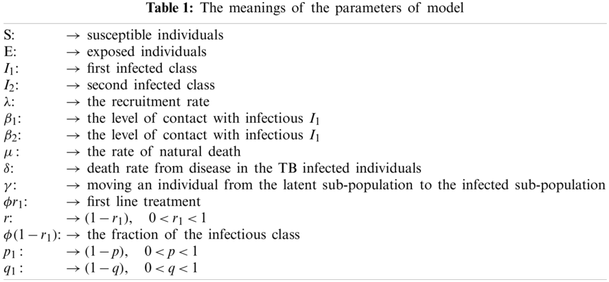
In this section, we will deal with numerical simulation of the Tuberculosis epidemic system of fractional stochastic differential equations. in order to demonstrate that the proposed method is effective and accurate. We have made use of the model with the piecewise differential operators and the numerical scheme where the Lagrange polynomial interpolation is used. In the numerical scheme, the first part is classical, the second part is fractional and last part is stochastic. We also present the results obtained from the fractional stochastic model, the numerical simulations are shown in Fig. 1 for alpha=1, Fig. 2 for alpha=0.5, Fig. 3 for alpha=0.6 and finally Fig. 4 for alpha=0.9 with density of randomness given by sigma1=0.01, sigma2=0.015, sigma3=0.012, sigma4=0.010. And with same alpha values but different density of randomness given by sigma1=0.1, sigma2=0.2, sigma3=0.3, sigma4=0.4 we put Figs. 5–8. Also figures including the initial conditions as
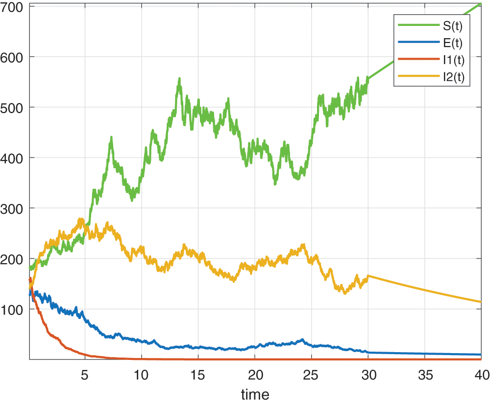
Figure 1: Numerical simulation for alpha=1
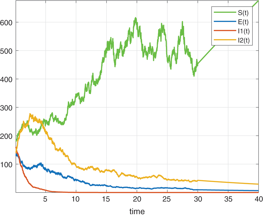
Figure 2: Numerical simulation for alpha=0.5
Figure 3: Numerical simulation for alpha=0.6

Figure 4: Numerical simulation for alpha=0.9
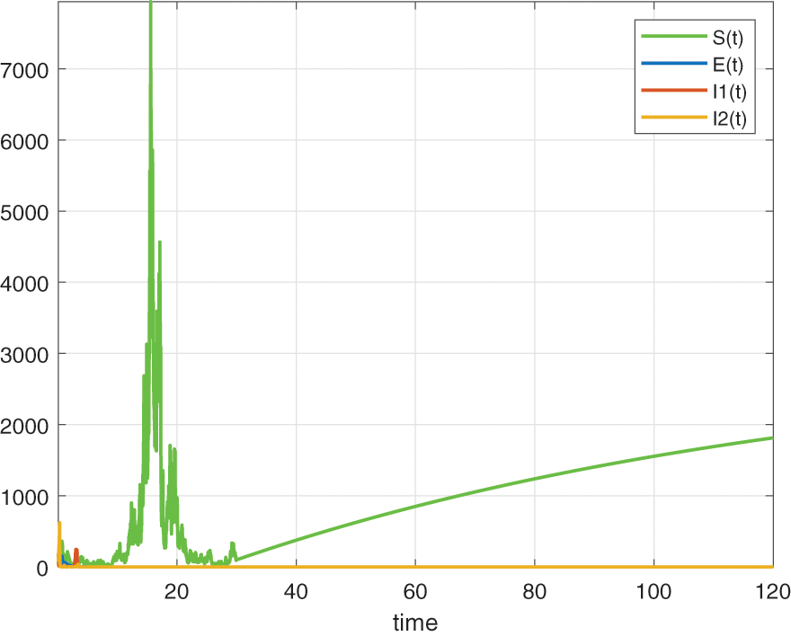
Figure 5: Numerical simulation for alpha=1
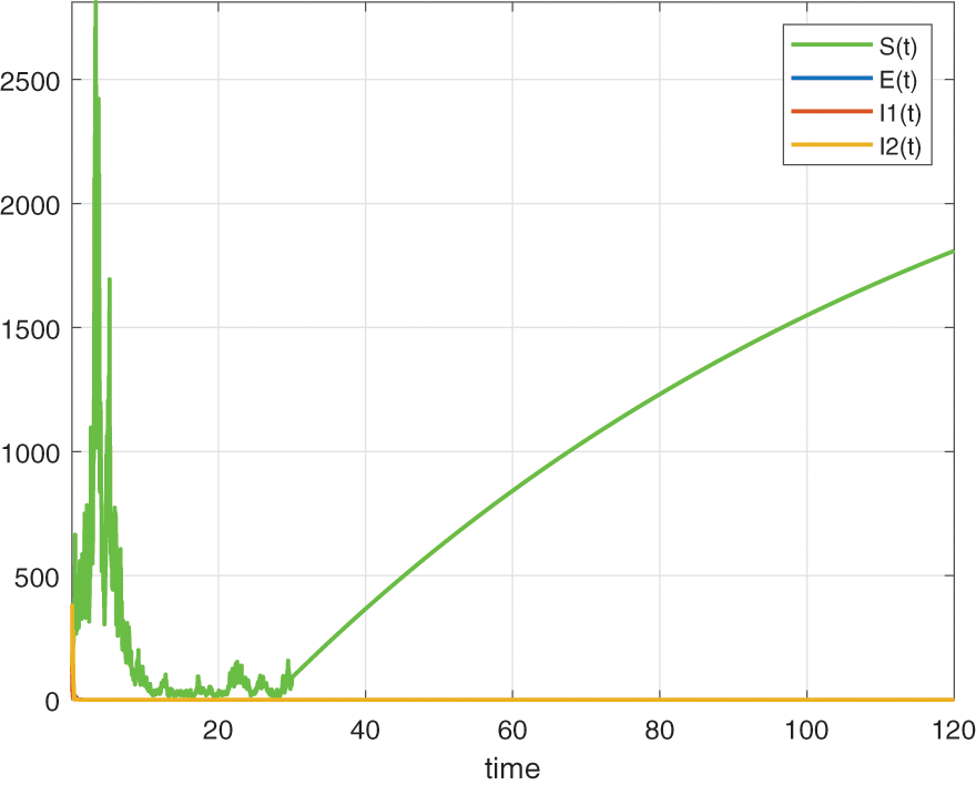
Figure 6: Numerical simulation for alpha=0.5
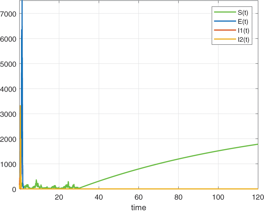
Figure 7: Numerical simulation for alpha=0.6
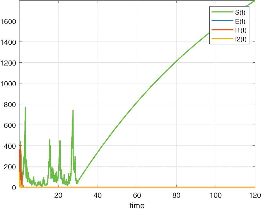
Figure 8: Numerical simulation for alpha=0.9
The spread of tuberculosis within human settlements and has infected and killed millions of humans in the last 200 years. While researchers from all backgrounds have put their efforts together to combat this virus and try to stop its spread, several studies have been performed; however, the virus is still spreading so far. Mathematical models are used to predict the future development of a given real-world problem. While several techniques and models have been proposed, they have not predicted piecewise behaviors of the spread. In this work, we attempted to present a model with piecewise patterns.
Funding Statement: The authors received no specific funding for this study.
Conflicts of Interest: The authors declare that they have no conflicts of interest to report regarding the present study.
1. Atangana, A., Araz, S. S. (2021). Modeling and forecasting the spread of COVID-19 with stochastic and deterministic approaches: Africa and Europe. Advances in Difference Equations, 2021(1), 1–107. DOI 10.1186/s13662-021-03213-2. [Google Scholar] [CrossRef]
2. Atangana, A. (2021). Mathematical model of survival of fractional calculus, critics and their impact: How singular is our world? https://hal.archives-ouvertes.fr/hal-03182789/document. [Google Scholar]
3. Nematollahi, M. H., Vatankhah, R., Sharifi, M. (2020). Nonlinear adaptive control of tuberculosis with consideration of the risk of endogenous reactivation and exogenous reinfection. Journal of Theoretical Biology, 486, 110081. DOI 10.1016/j.jtbi.2019.110081. [Google Scholar] [CrossRef]
4. Ogundile, O., Edeki, S., Adewale, S. (2018). A modelling technique for controlling the spread of tuberculosis. International Journal of Biology and Biomedical Engineering, 12, 131–136. [Google Scholar]
5. Atangana, A., Baleanu, D. (2016). New fractional derivatives with nonlocal and non-singular kernel: Theory and application to heat transfer model. Thermal Science, 20(2), 763. DOI 10.2298/TSCI160111018A. [Google Scholar] [CrossRef]
6. Caputo, M., Fabrizio, M. (2017). On the notion of fractional derivative and applications to the hysteresis phenomena. Meccanica, 52(13), 3043–3052. DOI 10.1007/s11012-017-0652-y. [Google Scholar] [CrossRef]
7. Caputo, M. (1967). Linear models of dissipation whose Q is almost frequency independent–II. Geophysical Journal International, 13(5), 529–539. DOI 10.1111/j.1365-246X.1967.tb02303.x. [Google Scholar] [CrossRef]
8. Dokuyucu, M. A. (2020). Caputo and atangana-baleanu-caputo fractional derivative applied to garden equation. Turkish Journal of Science, 5(1), 1–7. [Google Scholar]
9. Dokuyucu, M. A., Celik, E. (2021). Analyzing a novel coronavirus model (COVID-19) in the sense of caputo-fabrizio fractional operator. Applied and Computational Mathematics, 20(1), 49–69. [Google Scholar]
10. Ilknur, K., AKçetin, E., Yaprakdal, P. (2020). Numerical approximation for the spread of siqr model with caputo fractional order derivative. Turkish Journal of Science, 5(2), 124–139. [Google Scholar]
11. Dokuyucu, M. A. (2020). Analysis of a fractional plant-nectar-pollinator model with the exponential kernel. Eastern Anatolian Journal of Science, 6(1), 11–20. [Google Scholar]
12. Atangana, A., Araz, S. S. (2021). New concept in calculus: Piecewise differential and integral operators. Chaos, Solitons & Fractals, 145, 110638. DOI 10.1016/j.chaos.2020.110638. [Google Scholar] [CrossRef]
13. Qomariyah, N., Herdiana, R., Utomo, R., Permatasari, A. (2021). Stability analysis of a tuberculosis epidemic model with nonlinear incidence rate and treatment effects. Journal of Physics: Conference Series. 1943(1). 012118. [Google Scholar]
14. https://en.wikipedia.org/wiki/second_derivative. [Google Scholar]
 | This work is licensed under a Creative Commons Attribution 4.0 International License, which permits unrestricted use, distribution, and reproduction in any medium, provided the original work is properly cited. |