Computer Modeling in Engineering & Sciences

DOI: 10.32604/cmes.2022.019612

ARTICLE

Prototypical Network Based on Manhattan Distance

Zengchen Yu1, Ke Wang2,*, Shuxuan Xie1, Yuanfeng Zhong1 and Zhihan Lv3

1College of Computer Science and Technology, Qingdao University, Qingdao, China
2Psychiatric Department, Qingdao Municipal Hospital, Qingdao, China
3Qingdao Institute of Bioenergy and Bioprocess Technology, Chinese Academy of Sciences, Qingdao, China
*Corresponding Author: Ke Wang. Email: kw123456202111@163.com
Received: 01 October 2021; Accepted: 09 November 2021

1  Introduction

Deep Learning, or Deep Neural Network, is an important branch of artificial intelligence. It comes from the neuron computing model MP proposed by McCulloch et al. [1] in 1943. In 1958, Rosenblatt proposed the concept of a perception and proposed an algorithm close to human brain learning. This is the prototype of neural networks. In 1985, Geoffrey Hinton, the “originator of Deep Learning”, proposed a multilayer perception and improved the Back Propagation algorithm of neural networks [2]. Lecun et al. [3] adopted Convolutional Neural Network (CNN) to identify handwritten characters of postcodes in letters, achieving high accuracy. However, this algorithm was trained on the training set for 3 days, because the computer was not strong enough to effectively support neural network calculation at this time, so the Deep Neural Network fell silent for a time. In 2006, with the development of large-scale parallel computing and GPU, neural networks ushered in the third climax, and Deep Learning has become a hot spot in Artificial Intelligence. It is widely used in various fields, including face recognition, autonomous driving, search engines, health care, social network analysis, audio and voice processing, etc. Alzubaidi et al. [4] have greatly promoted the development of Artificial Intelligence.

However, Deep Learning also has some shortcomings. It is suitable for large-scale data and requires a large amount of data training model [5] in order to make full use of the advantages of parallel computing and GPU. However, for medical images, terrorist monitoring and other fields, it is impossible to obtain a large amount of data, or to obtain a large amount of data requires huge labor and cost [6], which is almost impossible [7]. Small-scale training data is prone to severe over-fitting.

Solving this problem can be inspired by the human learning process [8]. Humans can quickly learn from a small amount of data. For example, a five or six-year-old child has not seen a rhino, but after giving him a photo of a rhino, he can recognize it in many animal pictures. This is Few-shot Learning (FSL). In recent years, many scholars have been studying Few-shot Learning. Wang et al. [9] defined Few-shot Learning: Few-shot Learning is a machine learning problem (consisting of E(experience), T(task), and P(performance measurement) designation), where E contains only a limited number of examples of supervision information with target T. Or it can be said that the purpose of Few-shot Learning is to minimize the generalization error in the task distribution with few training examples [10]. The classification problem in Few-shot Learning usually uses the N way K shot method to divide the data: that is, metadata is divided into tasks instead of samples, and each task is internally divided into training set and test set, which are called support set and query set respectively. For each task, N classes (way) are randomly selected from the metadata set, and K (Shot) + 1 or K + M samples are randomly selected from each class. N*K samples are given to the support set for training, and the remaining N*1 or N*M samples are given to the query set for verification testing [11].

There are many ways to solve Few-shot Learning (here we mainly research the image field): (1) Model fine-tuning, training the model on a source dataset containing a large number of samples, and then fine-tuning the target dataset containing a small number of samples. If the source dataset and the target dataset are similar, this method can be used. But in actual scenarios, the two datasets are usually not similar, which often leads to over-fitting. (2) Data Augmentation, it refers to the use of some additional datasets or information to expand the target and the features of the dataset or augmentation of the samples in the target dataset. In the early time, it was achieved through spatial transformation, that is, the image was rotated, translated, cropped, and zoomed to expand the dataset, but this did not expand the types of samples. Later, people gradually began to use algorithms such as Generative Adversarial Network (GAN) for Data Augmentation. (3) Meta Learning, or, learning to learn, refers to letting the model have a certain learning ability, learn meta-knowledge from a large number of tasks, and use the meta-knowledge to quickly adapt to different new tasks. Meta Learning has algorithms such as Memory Neural Network, Meta Network, and MAML. (4) Metric Learning, also called similarity learning, calculates the distance between two samples through a distance function, measures the similarity between them, and determines whether they belong to the same category. The Metric Learning algorithm is composed of an embedding module and a metric module. The embedding module converts the sample into a vector in the vector space. The metric module gives the similarity between the samples. Metric Learning is divided into Metric Learning based on fixed distance and Metric Learning based on learnable metrics. We willalso introduce the specific development history of the above methods in Section 2. Our research can be applied in medicine, Synthetic Aperture Radar (SAR) image recognition and other fields, so we will also list some research on SAR image recognition, especially in Few-shot Learning.

Although Metric Learning based on learnable metrics is the mainstream, there are still merits to the exploration of Metric Learning algorithms based on fixed distances. What this paper is going to research is the Prototypical Network in Metric Learning based on a fixed distance. The Prototypical Network maps the sample data in each category to a space, and calculates their mean value as the prototype of the category. Using Euclidean distance as the measurement function, through training, the distance between the sample data and the prototype of its type is the shortest, and the distance to the prototype of other types is farther. During the test, the distance between the test data and the prototype of each category is processed by softmax function, and the category label of the test data is judged by the output probability value. The rapid convergence of the Prototypical Network is one of the reasons why the Prototypical Network is selected in this paper. Compared with other models, it can converge after only more than 10,000 episodes. This paper will use different measurement functions to improve Prototypical Network and expect better performance, especially Manhattan distance instead of Euclidean distance, the Manhattan Prototypical Network is proposed, and the average pooling layer and Dropout are respectively introduced into the embedded module. The accuracy and cross entropy loss of the improved model were compared with MAML, Matching Network, Relation Network and Meta-SGD on miniImageNet datasets. The data type of miniImagenet dataset is shown in Fig. 1. It can be seen that this dataset is very complex and difficult to identify.

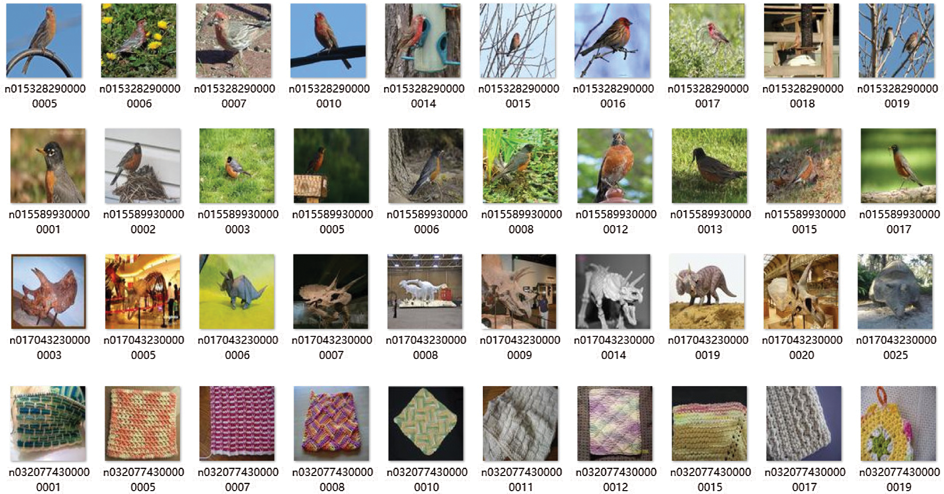
Figure 1: Screenshot of some categories of miniImageNet dataset (one category per line)

Section 2 of this paper will introduce in detail the historical development, advantages and disadvantages of model fine-tuning, Data Augmentation, Meta Learning, and Metric Learning. This section will list SAR related studies, too. Section 3 introduces and explains the principle and formula of the Prototypical Network, as well as our improvement on the core measure function and embedded module of the Prototypical Network. Section 4 explains the dataset, evaluation metrics, experimental procedures and experimental results. Section 5 summarizes the full text and puts forward prospects.

2  Related Work

2.1 Model Fine-Tuning

Model fine-tuning usually refers to training on a large-scale source dataset, and fine-tuning the parameters of the fully connected layer or top layers of the model on a small-scale target dataset. However, the source dataset and the target dataset need to be similar, otherwise the model cannot be used for fine-tuning. Because model fine-tuning is difficult to achieve cross-domain learning and easy to cause over-fitting, there is less research. Gidaris et al. [12] first trained a feature extractor with a large training set (the category in it is called the basic category). For the new few sample data, the attention mechanism is used to select the basic category weights for training. Nakamura et al. [13] pointed out that: 1) Using a low learning rate can stabilize the retraining process. 2) The use of an adaptive gradient optimizer during fine-tuning can improve the test accuracy. 3) When there is a large domain offset between the basic class and the new class, the test accuracy can be improved by updating the entire network. These methods achieve much higher accuracy than before on the miniImageNet dataset.

2.2 Data Augmentation

As mentioned in the introduction, the Data Augmentation method has been transformed from the early space transformation to the use of generative adversarial networks for data synthesis or feature augmentation.

The first is the data synthesis method. Mehrotra et al. [14] proposed the Generative Adversarial Residual Pairwise Networks, using Residual Neural Network to output the sample similarity of the support set and query set data. The loss of the GAN’s generator and discriminator is used to provide a strong regularized representation for the invisible data distribution to enhance similarity matching. Schwartz et al. [15] proposed Δ -encoder, which uses the Auto Encoder (AE) to find the deformation between different samples of the same category so that it can be applied to other categories to generate new samples. However, the feature augmentation of this method is too simple to effectively improve the classification boundary. There is also a combination of GAN and AE. Xian et al. [16] proposed the f-VAEGAN-D2 model, which combines the advantages of Variational Auto Encoder (VAE) and GAN.

Then introduce the feature augmentation methods. Dixit et al. [17] proposed Attribute Guided Augmentation (AGA), which learns synthetic features through the expected value of a set of object attributes (such as depth or pose). AGA can improve the recognition performance of a single object on a new class. Shen et al. [18] focused on adversarial features (features that cause the classifier to predict uncertainly), by adding an adversarial mask, forcing theclassifier to leave its comfort zone and focus on other areas for in-depth exploration, then use the overall feature map to learn more information.

However, augmentation is usually customized for each dataset and not easily transferable to other datasets, which is the problem to be solved in this direction.

2.3 Meta Learning

Meta Learning is to let the model learn, and let the model learn initially through a large number of tasks. When facing a new task, the model can complete the prediction task only by training a few times.

Santoro et al. [19, 20] used the Neural Turing Machine (NTM) as the basic model and proposed a memory augmentation network for One-shot Learning. NTM can either update the weights through a slow gradient descent to achieve the purpose of long-term memory, or through external storage. The module quickly binds information that has never been seen before to achieve short-term memory. In 2017, Munkhdalai et al. [21] proposed Meta Network, which divided the entire model into meta learner and base learner, and also included an external memory module to help fast learning. The base learner learns a specific task, and the meta-information loss gradient is given to the meta learner. Then the meta learner quickly learns and generalizes the new task.

The above methods are suitable for One-shot Learning. For Few-shot Learning, Finn et al. [22] proposed the MAML algorithm, which is independent of the model and is suitable for various learning tasks. Through a large number of task training, the model finds the best point. When facing a new task, it finds the optimal solution after a few steps of gradient descent update at this optimal point. MAML has been recognized by many scholars, and some scholars apply it to video scene anomaly detection, satellite data prediction, etc. [23, 24]. MAML requires second-order derivative calculations. In order to do only first-order operations, Nichol et al. [25] proposed Reptile, which uses the difference between the previous parameters and the parameters after K training to update. Reptile simplifies the calculation steps compared to MAML. But the performance is slightly degraded. MAML is very sensitive to the neural network architecture, it often leads to instability during training. It requires time-consuming and laborious hyper-parameter search to stabilize training and achieve high generalization, and the amount of calculation in training and inference time is very large, Antoniou et al. [26] proposed MAML++, which reduces the sensitivity of inner loop hyper-parameters, improves generalization errors, stabilizes and accelerates the MAML process. In addition to MAML, Li et al. [27] proposed Meta-SGD, which uses learning rate as an optimized parameter to perform gradient descent update, learn initialization parameters, update direction and learning rate. Or by combining Meta Learning with Transfer Learning, Jang et al. [28] proposed an effective training scheme for learning Meta Networks, which determines which layers between the source network and the target network should be matched for knowledge transfer and the amount of knowledge transfer in each feature.

Some build models through learning and optimization processes. Andrychowicz et al. [29] used LSTM to learn the parameter update process, dividing the parameters into different equal parts, each LSTM shared parameters, but did not share the hidden state; Ravi et al. [30] proposed a meta-learner model based on LSTM to learn an accurate optimization algorithm, which is used to learn another neural network classifier. The learning rate corresponds to the input gate in LSTM, the initialization parameter corresponds to the initializationvalue of the memory unit, an additional forget gate to supplement the coefficient of the last parameter in the gradient descent, and the use of parameter sharing to avoid parameter explosion.

Meta Learning algorithms need a lot of training tasks to acquire meta-knowledge, which is difficult to converge in a short time, so it is time-consuming.

2.4 Metric Learning

Metric Learning requires a similarity measurement function D(), similar samples get higher scores, and dissimilar samples get lower scores. This similarity measurement function can be a fixed distance or a learning network. The fixed distance metric is relatively simple, but limited by the situation, it is not easy to transfer to a new dataset. The learnable network metric can be applied to the new situation, but it is time-consuming to train. Metric Learning usually includes an embedding module and a metric module. The embedding module embeds the samples into the vector space. f() and g() respectively represent the embedding model that maps the support set and query set samples to the vector space, and its parameters are represented by θf and θg, respectively.

Koch et al. [31] proposed Siamese Neural Network, inputting pairs of samples (the same class of samples are labeled 1, and different classes are 0), and the same CNN is used to extract feature vectors for these pairs of samples, and then the distance measurement function is used to measure the distance between these pairs of feature vectors and input them into the sigmoid function to obtain the corresponding probability or similarity. In 2016, Vinyals et al. [32] proposed Matching Network. This network maps a small labeled support set and an unlabeled sample to the corresponding label, and uses LSTM to map the sample pair to a low-dimensional vector. Then use the kernel density estimation function to predict the unlabeled samples. As the size of the support set increases, each gradient update of the Matching Network becomes more expensive. When the label distribution has a significant deviation, the model will be affected. The above is mainly aimed at the single-sample problem. In order to better solve the Few-shot problem, Snell et al. [33] proposed Prototypical Network. Gao et al. [34] combined the attention mechanism and proposed Hybrid Attention Mechanism Network based on the Prototypical Network. The model has sample-level and feature-level attention mechanisms, respectively highlighting key sample instances and key features in the model. There is also a combination of Prototypical Network and Meta Learning. Wu et al. [35] proposed Meta-RCNN. First, a class prototype is constructed for each annotated object category in the support set, and the class-specific feature map of the entire image is constructed. The Region-Proposal Network (RPN), Few-shot Learning classifier and bounding box regressor are jointly trained in the Meta Learning framework. Das et al. [36] used Mahalanobis distance to propose a two-stage Few-shot Learning framework for image recognition.

In 2018, Sung et al. [37] proposed Relation Network and began to use learnable networks to replace fixed-distance modules. First construct an embedding unit to extract the feature information of each picture, connect the picture features to be tested and the picture features of the training samples and input them into the relation unit for comparison, then determine which category the test picture belongs to according to the comparison results. The Relation Network works well. Xiao et al. [38] used the Relation Network to segment and classify the Few-shot skin disease image. Zhang et al. [39] proposed a Deep Comparison Network (DCN) basedon a Relation Network. The network is composed of embedding and relation modules, which can simultaneously learn multiple nonlinear distance metrics based on features of different levels.

2.5 SAR

Wang et al. [40] proposed a new Few-shot Learning framework called Hybrid Inference Network (HIN) to solve the SAR target recognition problem with only a small number of training samples. The HIN identication process consists of two main stages. In the first stage, the embedding network is used to map the SAR image to the embedding space. In the second stage, a hybrid reasoning strategy combining inductive reasoning and transductive reasoning is used to classify the samples in the embedded space. In the inductive reasoning part, each sample is independently identified according to the metric based on Euclidean distance. Xue et al. [41] proposed a sequential SAR target classification method based on Spatial-Temporal Ensemble Convolutional Network (STEC-Net). In STEC-Net, the expanded 3D convolution is first applied to extract spatio-temporal features. Then, the features are gradually integrated hierarchically from local to global, and expressed as a joint tensor. Finally, a compact connection is applied to obtain a lightweight classification network. Wang et al. [42] proposed a new Few-shot Learning SAR ATR framework called Conv-BiLSTM Prototype Network (CBLPN) based on the embedded network.

3  Model Introduction

First, we present a representation of the dataset for a better description below. The N way K shot method is used to divide the data. The support set in a task includes N*K samples. If we use M instead of N*K, the support set can be expressed as follows: S = {(x1, y1), (x2, y2),… , (xM, yM)}, where xi is the D-dimensional feature vector, yi∈ {1, 2,… , N} means corresponding category, here we use Sk to represent the support subset of category k. The corresponding query set is represented by Q.

Next, we will separately introduce the embedded module and the measurement module of the improved Prototypical Network.

Firstly, the embedding module of the Prototypical Network converts all D-dimensional feature vectors in each support subset into Z-dimensional feature vectors in the new vector space through the embedding model f():

f:RD→RZ(1)

Here, a four-layer CNN is used as the embedding model f(), and Flatten layer is adopted for straightening. Its structure is shown in Fig. 2:

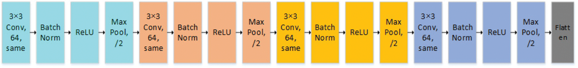
Figure 2: Embedded model CNN structure diagram

CNN are particularly suitable for extracting image features. Before CNN, Fully Connected Networks are generally used to extract image features. This causes the neural network to have a large number of connections and explode parameters, making it difficult to train. In fact, it is not necessary for each neuron to perceive the entire image. Image has a strong 2D local structure: spatially adjacent variables (or pixels) are highly correlated, so people put forward the concept of CNN, which combines three architectural ideas: local receptive fields, shared weights, and down sampling. The size of the convolution kernel is called the receptive field. The convolution kernel slides on the image to extract the features of its coverage area to achieve the purpose of forcibly extracting local features. At the same time, it can extract visual features such as edges and corners [43]. Since each area of the image is scanned by a convolution kernel with the same weight, weight sharing is realized and the number of parameters is saved. The convolutional layer of the CNN extracts local features well and avoids parameter explosion.

CNN also includes Batch Normalization layer, activation layer, and pooling layer. The Batch Normalization layer standardizes every batch of data to make it conform to the standard normal distribution, and performs scaling and offset, which effectively avoids the disappearance of the gradient, and can accelerate the speed of the gradient descent and accelerate the convergence. The activation layer performs nonlinear processing on the input through the activation function. It can be said that the activation function is one of the cores of the neural network, which can make the whole network fit any function. It can be said that the activation function is one of the cores of the neural network, it can make the entire network fit any function, the formula is as follows:

y=a(wx+b),(2)

where a() is the activation function, x is the input, and w and b are learnable weight parameters.

For hidden layers, ReLU activation function is generally used, because it has the advantages of avoiding gradient disappearance (in positive interval), fast calculation speed and fast convergence speed. The formula is as follows:

f(x)={0, if x≤0x, if x > 0(3)

The pooling layer [44] is a down-sampling layer that can extract invariant features, that is, features that remain unchanged under operations such as translation, rotation, and scaling. While preserving important features, it can reduce the number of data and parameters, avoid over-fitting, and improve the generalization performance of the model. Using the maximum pool layer, that is, taking the maximum value of the coverage area, can the extracted image texture and retain important details.

Then there is the measurement module. First, find the mean value of the Z-dimensional feature vector of each class in the new feature space, and get the prototype of each class. The formula is as follows:

Ck = 1|Sk|∑(xi,yi)∈Skf(xi)(4)

Here —Sk— represents the number of samples in Sk.

After finding the prototype, give the distance function D:RZ× RZ→ [0,+∞), and find the distance from the sample of the support set to each prototype. We will compare the effects of different distance functions in the experimental part. Here, we will list the distance functions to be compared. In the distance formula, —— represents the absolute value. Euclidean distance,

D(X,Y)=∑i=1n(xi−yi)2(5)

Here X = (x1, x2,… , xn) Y = (y1, y2,… , yn)

Manhattan distance, also known as city block distance, is the distance function that the model in this paper will ultimately adopt.

D(X,Y)=∑i=1n|xi−yi|(6)

Fig. 3 shows the graphical representation of Manhattan distance and Euclidean distance:

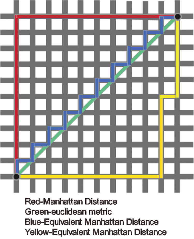
Figure 3: Manhattan distance, Euclidean distance diagram

In addition, Chebyshev distance,

D(X,Y)=maxi⁡|xi−yi|(7)

Cosine distance,

D(X,Y)=∑i=1n(xi×yi)∑i=1n(xi)2∑i=1n(yi)2(8)

After calculating the distance between sample x of query set Q and each prototype by distance function, the probability distribution is calculated by softmax function, which indicates the probability that x belongs to a prototype.

Pφ(y=k|x)=exp(−D(f(x),Ck))∑i=1nexp(−D(f(x),\; Ci))(9)

Here exp() represents an exponential function, and other parameters have been explained above. The category with the highest probability is output as the category to which the test data belongs.

Fig. 4 is a schematic diagram of the Prototypical Network under Few-shot Learning:

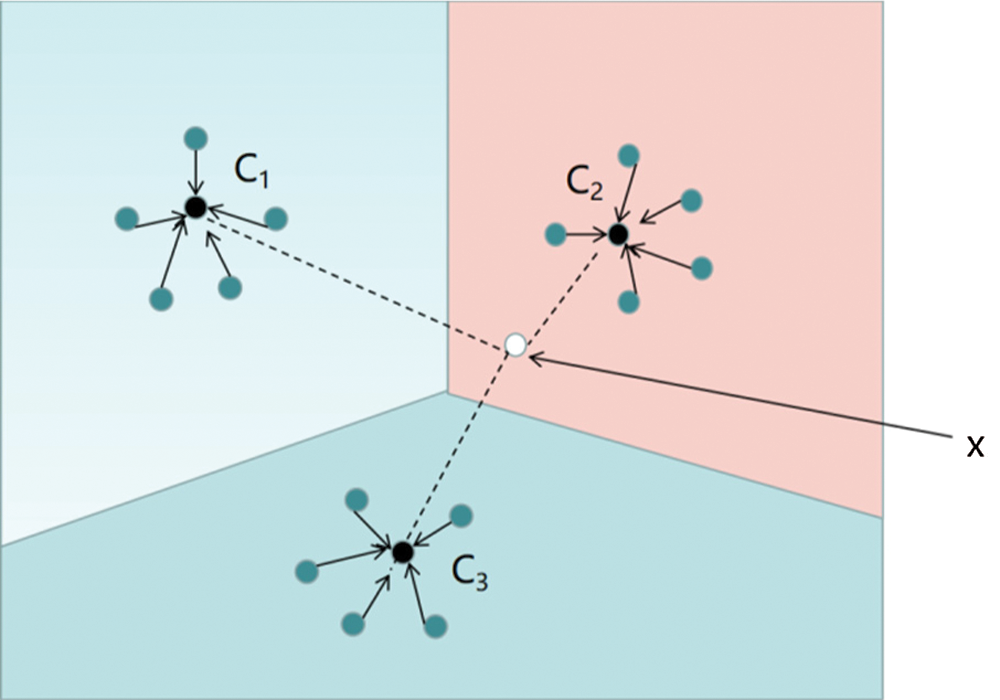
Figure 4: Schematic diagram of Prototypical Network under Few-shot Learning. The black circle (C1, C2, C3) represents the prototype of each class, and the white circle (x) represents the sample to be classified

The negative log probability of the true category k′ corresponding to the minimized sample is used for learning. The formula for this negative log probability is as follows:

J(φ)=−log⁡Pφ(y=|x)=D(f(x),Ck)+log⁡∑i=1nexp(−D(f(x),  Ci))(10)

This operation is equivalent to maximizing the probability distribution of the true category k′ corresponding to the sample.

The entire flow chart of the Manhattan Prototypical Network is given below in Fig. 5:

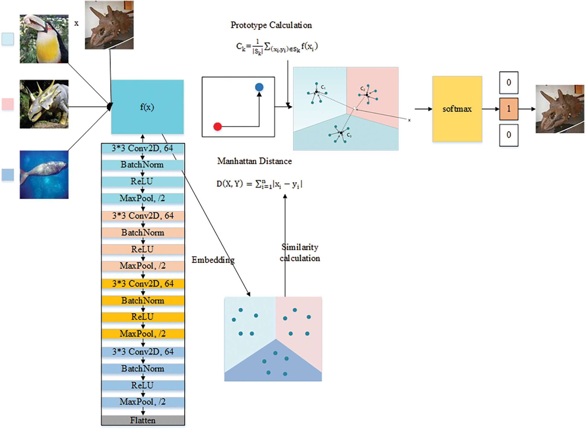
Figure 5: Overall flow chart of Manhattan Prototypical Network 1 (this picture explains the above process)

Or as shown in Fig. 6:

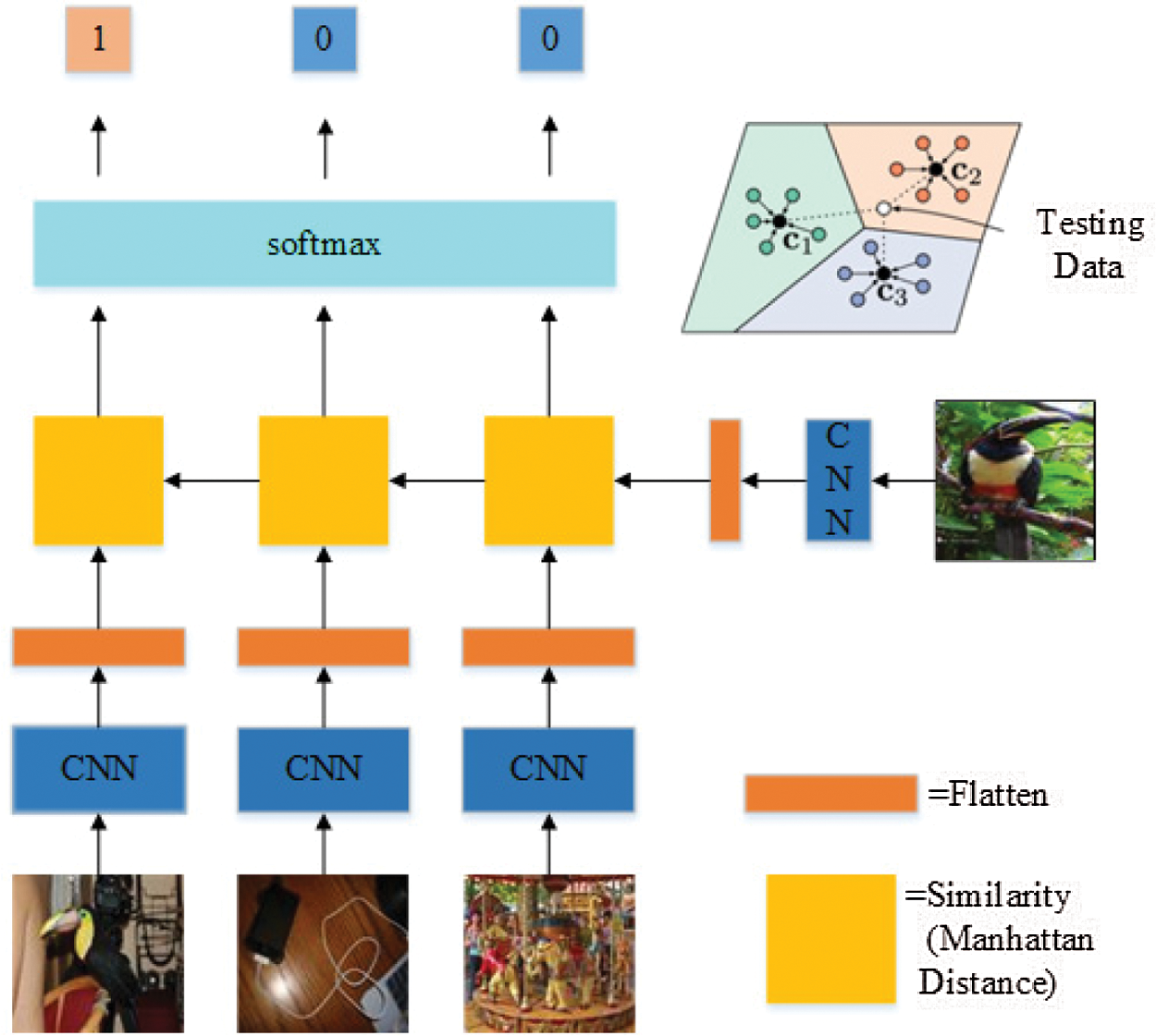
Figure 6: Overall flow chart of Manhattan Prototypical Network 2 (this picture explains the above process)

The Manhattan Prototypical Network is improved from the Prototypical Network, which also belongs to regular Bregman Divergences, which uses exponential family functions for density estimation.

The distance measurement part of Manhattan distance can be used to do the same derivation as the original text. The absolute value sign of the Manhattan distance can be cancelled by square.

d(f(x),  Ck)=|f(x)−Ck|(11)

|f(x)−Ck|2=f(x)−Ck=wkTf(x)−bk,wherewk=I,bk=Ck(12)

where wk and bk are weighted parameters, and I is the identity matrix.

This shows that the distance measurement part of the Manhattan Prototypical Network belongs to the linear model, and all the required nonlinearities are learned in the embedding function. This is the method currently used in modern neural network classification systems.

4  Experiments and Result

4.1 Dataset

The dataset used in this study is miniImageNet proposed by Vinyals et al. [32], which is the subset of the famous ILSVRC (ImageNet Large Scale Visual Recognition Challenge)-12 (ImageNet2012 dataset) [45]. ILSVRC-12 includes 1000 classes. There are more than 1000 samples in each category, which is very large. MiniImageNet selected 100 categories [46], including birds, animals, people, daily necessities, etc. Each category includes 600 84 * 84 RGB color pictures [47]. miniImageNet training is difficult, for Few-shot Learning, it still has very large development space. In this study, the dataset is simplified, and each class includes 350 samples. Among these 100 classes, we will randomly select 64 classes of data as the training set, 16 classes as the validation set, and the remaining 20 classes as the test set. We will mainly use the data division method of 5 way 5 shot and 5 way 1 shot for experiments.

4.2 Evaluation Metrics

Here we use the accuracy rate as the main evaluation metric, and the cross entropy loss as the auxiliary evaluation metric. We will apply evaluation metrics to the query set in the test set.

The concept of accuracy is relatively simple, that is, the ratio of the number of correctly classified samples m to the total number of samples n. The formula is as follows:

acc=mn(13)

The formula of cross entropy loss function is as follows:

L=1n∑i=1nLi=−1n∑i=1n∑j=1myijlog⁡pij(14)

Here, n represents the number of samples, m is the number of categories. yij represents 1 when the i-th sample belongs to category j, otherwise it is 0. pij represents the probability that the i-th sample is classified as category j [48], where pij is Eq. (10). Li represents the loss of the i-th sample. Eq. (14) is a convex function, and the global minimum can be obtained when deriving, and it is suitable as the loss function of the model.

4.3 Experimental Results

In this part, we will compare and tune models on the miniImageNet dataset. For the Prototypical Network and the improved Prototypical Network model used in this paper, namely Manhattan Prototypical Network, the same encoder–4-layer CNN is used to embed support and query points in the embedded part, and the initial learning rate is 0.001. The learning rate of episodes was halved per 2000, and Adam was used as the optimizer [49]. In order to show the rapid convergence of the model, 15,000 episodes (Each episode randomly selects samples to construct different support sets and query sets.) are basically used for iterative training for all experiments, and the accuracy and cross entropy loss are calculated by means of multiple test averages to reduce errors.

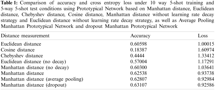
First, we use 10 way 5 shot for training and 5 way 5 shot for testing. Compare the accuracy and cross entropy loss of the Prototypical Network using Manhattan distance, Euclidean distance, Chebyshev Distance, Cosine Distance, Manhattan distance and Euclidean distance without learning rate decay strategy. During the experiment, we found that for changing the structure of the embedded module neural network-changing the maximum pooling layer to the average pooling layer or adding Dropout (This paper only adds the average pooling layer and Dropout layer to the first layer of the embedded module to avoid the degradation of model performance) will have good results. Add them to the Manhattan Prototypical Network for comparison (here in after referred to as the Average Pooling Manhattan Prototypical Network, the Dropout Manhattan Prototypical Network, or our model (Average Pooling), our model (Dropout)). This comparison is to obtain the optimal distance function and the improvement effect of the corresponding embedded module, test whether the improvement is effective, and verify the effect of the learning rate decay strategy. The results are shown in Table 1. The Manhattan distance and Euclidean distance have the best effect, and the accuracy can reach above 0.6. Manhattan distance has the highest accuracy rate, which is 0.0194 higher than Euclidean distance, and is close to 2%. Its cross entropy loss is the only one that is smaller than 1. It can prove that Manhattan distance is better than Euclidean distance, cosine distance, Chebyshev distance, and can exert greater performance. It can be found from the table that the accuracy of using the learning rate decay strategy is 0.02–0.03 higher than that of not using this strategy. The principle of learning rate decay strategy is that, in the early stage of learning, a larger pace is adopted to accelerate convergence, which requires a larger learning rate. In the later stage, the model begins to converge, which requires a smaller pace to avoid oscillation at the minimum value, and finally achieves convergence. Moreover, the accuracy of Average Pooling Manhattan Prototypical Network and Dropout Manhattan Prototypical Network is often higher.

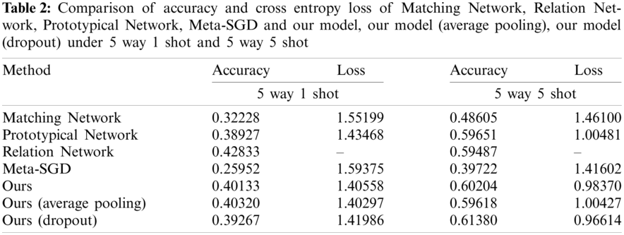
Then we compare the accuracy and cross entropy loss of the Matching Network, the Relation Network, the original Prototypical Network, the Meta-SGD model with our model (Manhattan Prototypical Network), our model (Average Pooling), our model (Dropout) with 5 way 5 shot and 5 way 1 shot, respectively. These models have been introduced in the Section 2. As shown in Table 2, under the condition of 5 ways 5 shot, it is found that the accuracy of Prototypical Network, Relation Network and our model under various improvements is over 0.59, and the accuracy of our models are over 0.6. Dropout improves the accuracy of Manhattan Prototypical Network by 1%, and the loss function is almost reduced below 1 except for the improvement of average pooling layer. Under the condition of 5 ways 1 shot, the performance of this model is second only to the Relation Network.

Under the setting of 15,000 episodes in this experiment, through training MAML and comparing with its original papers, it is found that it is far from reaching the convergence level, while Prototypical Network and improved Prototypical Network model can indeed guarantee convergence within 15,000 episodes, which is faster than other models. Here, under the training condition of 10 way 5 shot, the accuracy and cross entropy loss of MAML, Prototypical Network, Manhattan Prototypical Network, Average Pooling Manhattan Prototypical Network and Dropout Manhattan Prototypical Network are compared. We can see that the performance of these five is almost gradually improving, and the best one is Dropout Manhattan Prototypical Network.

It can be seen from Fig. 7 that the accuracy of Manhattan Prototypical Network and its improvement exceeds that of the original Prototypical Network and other models. Average Pooling Manhattan Prototypical Network and Dropout Manhattan Prototypical Network can play better classification effects than Manhattan Prototypical Network, especially Dropout Manhattan Prototypical Network can improve the accuracy by about 1%.

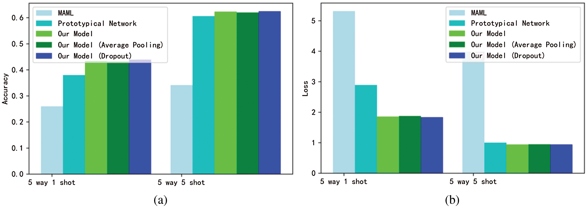
Figure 7: Performance comparison of MAML, Prototypical Network, Manhattan Prototypical Network, Average Pooling Manhattan Prototypical Network and dropout Manhattan Prototypical Network. (a) Accuracy; (b) Cross entropy loss

Adjust parameters and compare them by learning curves below:

Initial learning rate:

Generally, for Few-shot Learning algorithms, the initial learning rate is set to 0.001, but if it is set to other values, the effect will be reduced. For the initial learning rate, the Prototypical Network, our model, our model (Average Pooling) and our model (Dropout) are tested with the interval of 0.0001–0.011. As shown Fig. 8, it is found that when the initial learning rate is set to 0.001, the effect is the best. Too small and too large a learning rate will lead to poor model effect, especially when it is too large, sometimes the accuracy of Manhattan Prototypical Network and Prototypical Network model will fall below 0.2. However, the accuracy of Average Pooling Manhattan Prototypical Network and Dropout Manhattan Prototypical Network can be kept above 0.54.

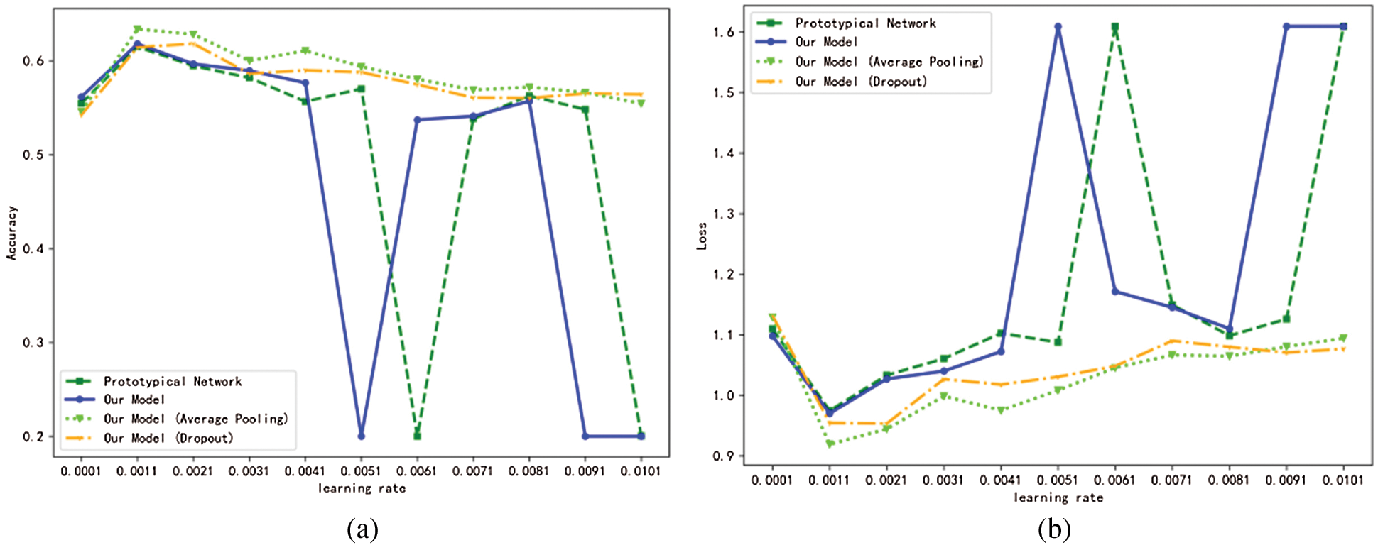
Figure 8: Use the 0.0001–0.011 interval for the learning rate (0.001 is the step size) to test the Prototypical Network and our model, our model (Average Pooling) and our model (Dropout). (a) Accuracy; (b) Cross entropy loss

Number of neural network layers:

The CNN of the Prototypical Network and our model are both set to 4, but if the number of layers is simply deepened or reduced, the performance of the model will be degraded, resulting in some degree of over-fitting and under-fitting. We set the CNN to 3, 4 and 5 layers respectively for testing. The result is shown in Fig. 9. When the number of layers of CNN is less than 4 and higher than 4, the network performance will be degraded, especially when the number of layers is higher than 5, the network performance will be degraded rapidly. This shows that only changing the number of layers will not improve the performance of the models.

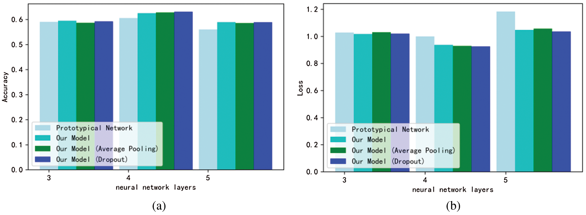
Figure 9: Comparison of the effects between Prototypical Network and our model, our model (Average Pooling) and our model (Dropout) when the number of neural networks is set to 3, 4 and 5. (a) Accuracy; (b) Cross entropy loss

Number of training categories:

According to the previous data, it can be found that the accuracy of the Prototypical Network with 10 training categories and Manhattan Prototypical Network is 0.01–0.02 higher than that of the Prototypical Network with 5 training categories. Is it possible to draw a conclusion that within a certain range, the more categories during training, the higher the model performance? It can be seen from Fig. 10 that it is not that the more training categories, the higher the model performance. For these two types of networks, when the number of training classes is 10 (for Euclidean distance) or 20 (for Manhattan distance), the model has the best accuracy and cross entropy loss. When the value is 20, the Manhattan distance Prototypical Network can even reach 0.63700, and the Average Pooling Manhattan Prototypical Network can reach more than 0.639, which is close to 0.64. When the number of training categories is higher than 20, the accuracy will decrease and the loss of cross entropy will increase.

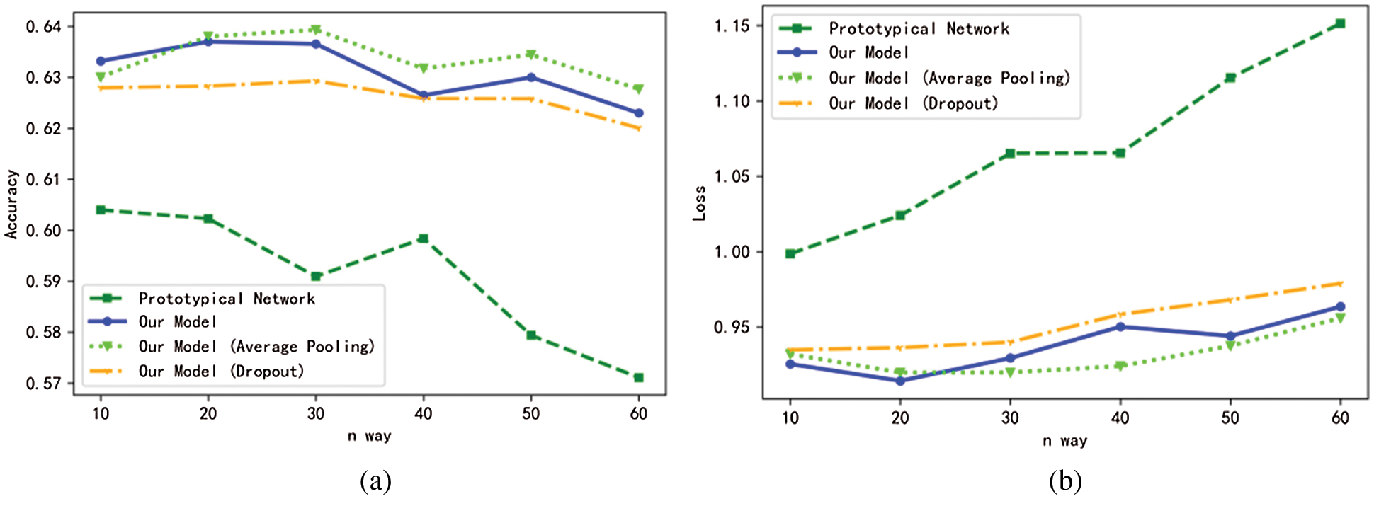
Figure 10: Accuracy and cross entropy loss curves of Prototypical Network and Manhattan Prototypical Network, Average Pooling Manhattan Prototypical Network and dropout Manhattan Prototypical Network when the number of training categories is 10–60 (step size is 10). (a) Accuracy curve; (b) Cross entropy loss graph

Number of convolution kernels in each layer of Neural Network:

By adjusting the number of convolution kernels in each layer of CNN, it is found that the number of convolution kernels is almost positively correlated with the performance of Prototypical Network and Manhattan Prototypical Network and their improvements. When the number of convolution kernels reaches 80, the accuracy of Manhattan Prototypical Network reaches 0.64733. When the number of convolution kernels is 128, the accuracy of Manhattan Prototypical Network remains above 0.642, and the accuracy of Prototypical Network is close to 0.62. It can be seen from Fig. 11 that Average Pooling Manhattan Prototypical Network, Dropout Manhattan Prototypical Network and Manhattan Prototypical Network have similar performance.

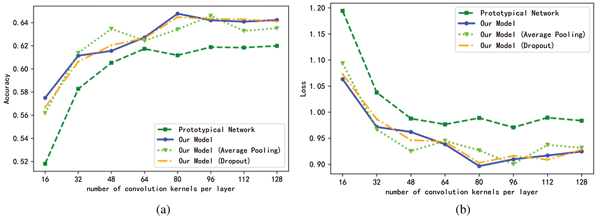
Figure 11: Accuracy and cross entropy loss curves of Prototypical Network, Manhattan Prototypical Network, Average Pooling Manhattan Prototypical Network and dropout Manhattan Prototypical Network when the number of convolution cores in each layer of neural network is 16–128 (step size is 16). (a) Accuracy curve; (b) Cross entropy loss curve

5  Conclusion

In this paper, an improved Prototypical Network is proposed, in which the core distance measurement function of the original Prototypical Network is changed from Euclidean distance to Manhattan distance, and the average pooling layer and Dropout layer are added respectively. The improved Prototypical Network has higher performance and convergence, exceeding the original Prototypical Network, MAML, Matching Network, Relation Network, Meta-SGD and Prototypical Network improved based on other distances within 15,000 episodes. The Manhattan Prototypical Network with the average pooling layer and Dropout was better at times, especially with the addition of Dropout. After parameter adjustment, the performance of the model can reach 0.64733. This means that the Manhattan distance is more suitable for Prototypical Network, and exceeds the Euclidean distance and Cosine distance explored in the original paper and other metric measurements. It has higher stability than other measures in some cases. Combining the coding layer and classification layer of the model, the parameters are less and the training is more convenient. In specific experiments, the concept of “Prototype” is only used in the function part of calculating the loss of the model, while the backbone network of the model is not disturbed, which means that the portability and extensibility of the Prototypical Network are also excellent. This research determined the better metric function–Manhattan distance in the fixed distance metric in the Metric Learning of Few-shot Learning and adds the average pooling layer and Dropout layer to improve the performance. There are often fewer samples in the field of medicine and SAR. Applying our research to medicine and SAR can play a better effect than other models listed in this paper. In the future, we will try to apply other complex CNN to it, and we can also explore Metric Learning based on learnable metrics to improve the performance of Few-shot Learning algorithms.

Funding Statement: The authors received no specific funding for this study.

Conflicts of Interest: The authors declare that they have no conflicts of interest to report regarding the present study.

This work is licensed under a Creative Commons Attribution 4.0 International License, which permits unrestricted use, distribution, and reproduction in any medium, provided the original work is properly cited.