| Computer Modeling in Engineering & Sciences |
DOI: 10.32604/cmes.2022.019754
ARTICLE
Two-Machine Hybrid Flow-Shop Problems in Shared Manufacturing
Ningbo University of Finance & Economics, Ningbo, 315175, China
*Corresponding Author: Qi Wei. Email: weiqi@nbufe.edu.cn
Received: 13 October 2021; Accepted: 01 November 2021
Abstract: In the “shared manufacturing” environment, based on fairness, shared manufacturing platforms often require manufacturing service enterprises to arrange production according to the principle of “order first, finish first” which leads to a series of scheduling problems with fixed processing sequences. In this paper, two two-machine hybrid flow-shop problems with fixed processing sequences are studied. Each job has two tasks. The first task is flexible, which can be processed on either of the two machines, and the second task must be processed on the second machine after the first task is completed. We consider two objective functions: to minimize the makespan and to minimize the total weighted completion time. First, we show the problem for any one of the two objectives is ordinary NP-hard by polynomial-time Turing Reduction. Then, using the Continuous Processing Module (CPM), we design a dynamic programming algorithm for each case and calculate the time complexity of each algorithm. Finally, numerical experiments are used to analyze the effect of dynamic programming algorithms in practical operations. Comparative experiments show that these dynamic programming algorithms have comprehensive advantages over the branch and bound algorithm (a classical exact algorithm) and the discrete harmony search algorithm (a high-performance heuristic algorithm).
Keywords: Hybrid flow-shop; dynamic programming algorithm; computational complexity; numerical experiments; shared manufacturing
In this paper, we study two two-machine hybrid flow-shop scheduling problems with fixed processing sequences. In this problem, a set of n jobs
Hybrid flow-shop problems are widely used in the traditional manufacturing industry [1], computer graphics processing [2], medical operation scheduling [3], and other fields. For the research on the hybrid flow-shop problem, please refer to the latest review [4]. A typical application scenario of the two-stage hybrid flow-shop scheduling is as follows. In integrated circuit manufacturing or mechanical manufacturing, product processing usually includes two stages: preliminary processing and finishing processing. The factories are equipped with two sets of equipment, one set of low-precision equipment for preliminary processing and the other set of high-precision equipment for finishing processing. However, when necessary, the high-precision equipment can also be degraded for preliminary processing. Reasonably arrange the processing sequence and processing machines can make all products complete as soon as possible.
The scheduling problems with fixed processing sequences refer to the scheduling problem in which the processing order of the jobs is determined in advance. This kind of problem is originally mainly applied to the stock control systems [5]. In recent years, with the integration of the sharing economy into the traditional manufacturing industry, there has been a shared manufacturing mode that shares manufacturing resources and demands on the network platform and matches supply and demand through advanced algorithms [6]. “Alibaba Taobao Factory” and “Aerospace Cooperative Manufacturing Network” in China, “Wanju-gun Local Food Processing Center” in Korea, and many other share manufacturing practices have been vigorously developed. Based on fairness, shared manufacturing platforms often require manufacturing service enterprises to arrange production according to the principle of “order first, finish first” which forms a constraint of fixed processing sequences. Suppose the two-stage hybrid flow-shop scheduling problem with two machines described above is considered in the shared manufacturing environment. It is equivalent to adding the constraint of fixed processing sequences in the above typical application scenario. Obviously, the mathematical model of this problem is the scheduling model described in the first paragraph of this section.
1.2 Related Problems and Results
Wei et al. [2] first considered this two-stage hybrid flow-shop scheduling problem without fixed processing sequences constraint (denoted by SHFS) in 2005. They proved that this problem is ordinary NP-hard and presented an approximation algorithm with polynomial-time computational complexity whose worst-case ratio is 2. For the same problem, Jiang et al. [7] designed an improved approximation algorithm whose worst-case ratio is 1.5. Recently, for the case where every job has a deadline and must be processed in a given order, Wei et al. [8] proposed efficient algorithms.
The research results of other hybrid flow-shop scheduling problems with two stages close to the problems studied in this paper are as follows. A special hybrid flow-shop scheduling problem with two machines was considered by Vairaktarakis et al. [1]. In their problem, the two tasks of each job can be processed on any one of the two machines, i.e., there are four processing methods in total. An excellent approximate algorithm was presented whose worst-case ratio is only 1.618. Zhang et al. [9] studied another similar problem where the later task of each job can be jointly processed by multiple machines, but the former task cannot. An approximate algorithm was presented in their paper whose worst-case ratio is only
The earliest scheduling problem with fixed processing sequences was presented by Shafransky et al. [22]. They considered the model with fixed processing sequences in an open-shop problem, showed this problem is NP-hard in the strong sense, and proposed a very accurate polynomial-time approximate algorithm whose worst-case ratio is only 1.25. Lin et al. [5] studied a two-stage differentiation flow-shop to minimize the total completion time and proposed a dynamic programming algorithm. Hwang et al. [23,24] firstly studied the general two-machine flow-shop problem with a given sequence and presented an optimal algorithm for each of the two special cases. Then, they studied the general flow-shop scheduling with batching machines and proposed optimal algorithms for several models. With the gradual emergence of the application value of the scheduling problem with fixed processing sequences, the related research has increased a lot in recent years. Lin et al. [25] considered a relocation scheduling problem with fixed processing sequences corresponding to resource-constrained scheduling on two parallel dedicated machines. They proposed polynomial-time optimal algorithms or approximate algorithms for several models with different objective functions. Halman et al. [26] further gave a fully polynomial-time approximation scheme for the above problem. Cheref et al. [27] studied a scheduling problem considering production and delivery with a given sequence. They showed that this problem is NP-hard and proposed a dynamic programming algorithm with good effect. A server scheduling problem on parallel dedicated machines with fixed processing sequences was considered by Cheng et al. [28,29]. For the two-machine case, a polynomial-time approximation algorithm was presented; for the case where each loading time is unit, two heuristic algorithms were proposed; and for the general case, a pseudo-polynomial algorithm was presented. However, the two-stage hybrid flow-shop scheduling with fixed processing sequences and the goal of minimizing makespan or total weighted completion time has not been considered yet.
In the “shared manufacturing” environment, we introduce the constraint of fixed processing sequences into the two-machine two-stage hybrid flow-shop scheduling problem SHFS. We consider two objectives of this problem: to minimize the makespan and to minimize the total weighted completion time. For each problem, we analyze the computational complexity and present a dynamic programming algorithm. According to the three-field representation, these two problems can be expressed in the following form:
(1)
(2)
which are denoted by SHFSFC and SHFSFW.
Firstly, we give the structural characteristics of one optimal solution and prove that these two problems are both ordinary NP-hard. Then we propose the dynamic programming algorithms and calculate their time complexity. Finally, we show the advantages of these algorithms over the existing exact algorithms and heuristic algorithms in practical efficiency and effect by numerical experiments.
The rest of this paper is arranged as follows: In Section 2, we first give the basic symbolic assumptions and the characteristics of one optimal solution, then analyze the computational complexity of the problems; In Sections 3 and 4, the dynamic programming algorithms for SHFSFC and SHFSFW are proposed, respectively; In Section 5, we compare the dynamic programming algorithms presented in this paper with the existing algorithms through numerical experiments to obtain the actual efficiency and effect of these algorithms. Finally, we conclude the paper and give the future research ideas in Section 6.
2 Symbolic Assumptions, Structure of One Optimal Schedule, and Complexity of the Problems
The basic symbols to be used in the following are given, properties of one optimal schedule of SHFSFC (SHFSFW) are analyzed, and the computational complexity of each problem is proved in this section.
The symbols and their meanings to be used below are as follows:
•
•
•
•
•
•
2.2 Structure of Optimal Scheduling
The two problems studied in this paper do not consider the buffer capacity between the two stages. That is, the buffer capacity is deemed to be infinite. So the tasks processed on machine
From the above analysis, it is easy to find that the following proposition holds whether the objective is to minimize makespan or total weighted completion time.
Proposition 2.1 There exists one optimal schedule of SHFSFC (SHFSFW) that satisfies the following properties at the same time:
(1) Task
(2)
(3) There is no idle time on
(4) There is no idle time on
Proof:
(1) Suppose
(2) Suppose
(3) Suppose
(4) Suppose
To sum up, we can get Proposition 2.1 holds.
According to Proposition 2.1, it is easy to obtain there exists an optimal schedule of SHFSFC (or SHFSFW), which is shown in Fig. 1 below. That is, there exists an optimal schedule of SHFSFC (or SHFSFW) in which
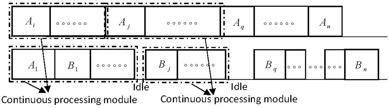
Figure 1: The structure of an optimal schedule
2.3 Computational Complexity of the Problems
Next, we prove that SHFSFC and SHFSFW are both NP-hard by Turing Reduction.
Theorem 2.2 Problem SHFSFC is NP-hard, even if the processing time of the second task of every job is 0, i.e.,
Proof: First, propose an Instance I of a well-known NP-hard problem Partition Problem: There is a set of n integers
Then, based on Instance I, we construct an Instance II of SHFSFC: There is a job set of
(1)
(2)
(3)
Is there a feasible schedule of Instance II that makes makespan
Now, let's prove that the solutions of Instances I and II can be derived from each other. Suppose
Suppose (
Next, we prove that
Considering that
It is known that Partition Problem is NP-hard, so it is easy to have that SHFSFC is also NP-hard.
Obviously, the above proof process still holds when
Theorem 2.3 SHFSFW is NP-hard.
Proof: Considering that the jobs are processed in subscript order, we have
3 A Dynamic Programming Algorithm of Problem SHFSFC
According to Proposition 2.1, there is an optimal schedule of Problem SHFSFC, which is composed of several continuous processing modules and the idle times between continuous processing modules. Therefore, the following dynamic programming algorithm includes two stages: Construct the optimal continuous processing modules and connect the optimal continuous processing modules through idle times to form an optimal schedule. Firstly, the strict definition of continuous processing module for SHFSFC is given:
Definition 3.1 A sub-schedule consisting of a job subset
(1) The first task of job
(2) No matter on
(3) The difference between the complete time of subset
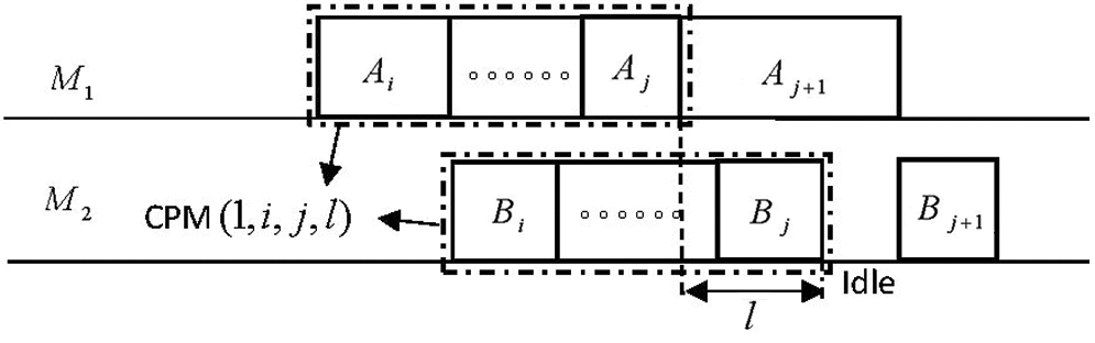
Figure 2: The continuous processing module(
It is easy to see that CPM
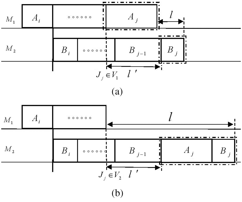
Figure 3: The two ways from CPM(
For the convenience of narration, a symbolic function is defined below:
Definition 3.2 Symbolic function
When
In the following discussion, we let
Obviously, in the sub-schedule composed of job subset
Dynamic Programming Algorithm CPM(C):
Initial Conditions:
Recurrence Relation:
The parameters
(1) When
(2) When
Recurrence Formula:
The initial conditions and recurrence formula in dynamic programming algorithm CPM(C) are clearly valid. So we mainly analyze the recurrence relation below. Given a set of required parameters
After the optimal continuous processing modules are constructed, the whole schedule can be constructed by recursively connecting these optimal continuous processing modules. It should be noted that every two continuous optimal continuous processing modules are separated by an idle time on
Dynamic Programming Algorithm DP(C):
Initial Conditions:
Recurrence Relation:
The parameters
Recurrence Formula:
Target Value:
The initial conditions, recurrence formula, and target value in dynamic programming algorithm DP(C) are clearly valid. So we also mainly analyze the recurrence relation below. When the optimal CPM
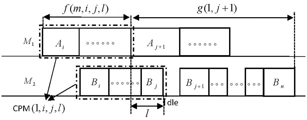
Figure 4: From CPM
Theorem 3.3 Dynamic programming algorithm DP(C) is a pseudo-polynomial time algorithm, and its time complexity is
Proof: Firstly, we consider the time complexity of solving the optimal continuous processing module. It takes
Since SHFSFC has a pseudo-polynomial time algorithm, SHFSFC is ordinary NP-hard. That is, the following theorem holds.
Theorem 3.4 Problem SHFSFC can be solved in
4 A Dynamic Programming Algorithm of Problem SHFSFW
This section will construct a dynamic programming algorithm for problem SHFSFW using a method similar to Section 3. First, we construct the optimal continuous processing modules and calculate the objective value of every optimal continuous processing module by a dynamic programming algorithm. Then, we use optimal continuous processing modules to construct an optimal partial schedule. Finally, the objective of the optimal schedule is calculated by backward recursion. However, the goal of SHFSFW is to minimize the total weighted completion time, which is different from makespan. It has no direct relationship with the load of the jobs on machine
Definition 4.1 A sub-schedule consisting of a job subset
(1) The first task of job
(2) No matter on
(3) The load generated by the subset
(4) The difference between the complete time of subset
It is easy to see that CPM
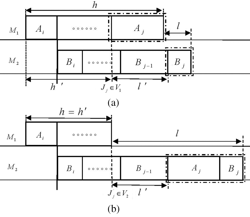
Figure 5: The two ways from CPM(
Dynamic Programming Algorithm CPM(WC):
Initial Conditions:
Recurrence Relation:
The parameters
(1) When
(2) When
Recurrence Formula:
Next, we define the Partial Schedule
Dynamic Programming Algorithm DP(WC):
Initial Conditions:
Recurrence Relation:
The parameters
Recurrence Formula:
Target Value:
The initial conditions, recurrence formula, and target value in dynamic programming algorithm DP(WC) are clearly valid. So we also mainly analyze the recurrence relation below. Once the optimal CPM
Through the analysis similar to Theorem 3.3 in Section 3, we can obtain the following theorem on the time complexity of dynamic programming algorithm DP(WC).
Theorem 4.2 Dynamic programming algorithm DP(WC) is a pseudo-polynomial time algorithm, and its time complexity is
Similar to Theorem 3.4, we can have the following theorem.
Theorem 4.3 Problem SHFSFC can be solved in
5 Analysis of Algorithm Effect Based on Numerical Experiments
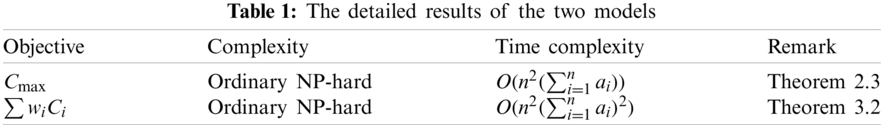
We analyze the computational complexity of two problems, design dynamic programming algorithms for them, and calculate the time complexity of the algorithms in Sections 2–4. These results are summarized in Table 1.
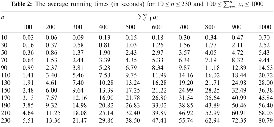
We took SHFSFC as an example to test the operation efficiency of the dynamic programming algorithms designed in this paper through numerical experiments. The numerical experiments were carried out in Matlab R2017 on a laptop with built-in an Intel Core i5 8250u CPU, 8 GB LPDDR3 RAM, and Windows 10. The processing time of each flexible task
It can be seen from Table 2 that even if n reaches 230 and the total processing time of all flexible tasks reaches 1000, the time used by algorithm DP(C) only needs less than 85 s. Therefore, we can conclude that the actual effect of the algorithm is entirely acceptable.
Using the data in Table 2, we can discuss the relationship between the running time of the algorithm and the total processing time of all flexible tasks when there are fewer jobs (
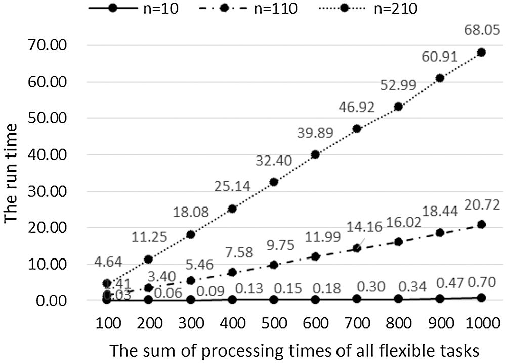
Figure 6: When
Similarly, the data in Table 2 is used to analyze the relationship between the running time of the algorithm and the number of jobs when the total processing time of all flexible tasks is small (
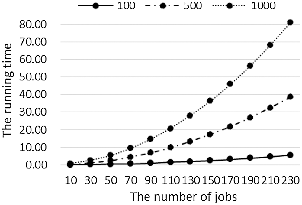
Figure 7: When
5.2 Comparison with Other Commonly Used Algorithms
Since there is no other algorithm for the two-stage hybrid flow-shop problem studied in this paper, we compare the high-quality algorithms for a similar problem with the dynamic programming algorithms given in this paper to analyze the effect of our algorithms.
We usually design polynomial-time optimal algorithms to solve P problems [30]. But there exist two kinds of algorithms for solving NP-hard problems. The first one is the exact algorithm, which gives the optimal solution, but the time complexity is exponential, including the enumeration algorithm, branch and bound algorithm [31]. The second one is the heuristic algorithm, which usually gives the approximate solution of the problem, but the time complexity is polynomial, including the genetic algorithm [20,32], (Iterated) green algorithm [33], fireworks algorithm [34], artistic neural network algorithm [35], (discrete) harmony search algorithm [36], etc. These algorithms are widely used in solving various scientific and engineering problems. From the analysis of the existing literature, it is found that the branch and bound algorithm is the most commonly used and relatively practical algorithm in the accurate solution of hybrid flow-shop problems [31,37]. Regarding the heuristic algorithm, the research in literature [36] shows that a discrete harmony search algorithm has advantages compared with a genetic algorithm, greedy algorithm, and harmony search algorithm, both in running time and the average relative percentage deviation, in solving hybrid flow-shop problems. The average Relative Percentage Deviation (denoted by RPD) is usually used to measure the approximation of heuristic algorithms [38], and its specific definition is as follows:
We still took problem SHFSFC as an example to compare dynamic programming algorithm DP(C) (the algorithm given by us), the branch and bound algorithm (given by Moursli et al. [31], denoted by B&B), and the discrete harmony search algorithm (given by Zini et al. [36], denoted by DHS) regarding the running time and the average relative percentage deviation.
The numerical experiments were carried out in the same software and hardware environment as in Section 5.1. The time complexity of B&B and DHS is independent of
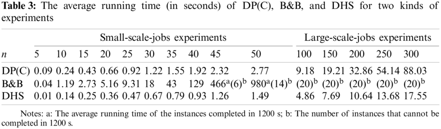
As shown in Table 3, DP(C) and DHS can complete the operation in 100 s in both two cases. In particular, DHS can be completed in 20 s, showing its advantage in time complexity. However, for B&B, when the number of jobs reaches 45, some instances cannot be completed in 1200 s; when the number of jobs reaches 50%, 70% of the instances cannot be completed in 1200 s; and all large-scale-jobs experiments cannot be completed in 1200 s.
The relationship between running time and n of each algorithm in the small-scale-jobs case is shown in Fig. 8. For this case, we can get that: (1) DHS has the most advantage in time complexity, followed by DP(C), while B&B has obvious disadvantages; (2) The running time of each algorithm increases with the increase of the number of jobs and one of B&B increases much faster than the other two algorithms.
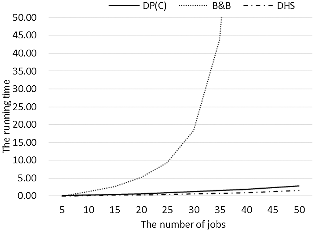
Figure 8: The average running time of DP(C), B&B, and DHS for small-scale-jobs experiments
Similarly, using the data in Table 3, the relationship between running time and n of each algorithm in the large-scale-jobs case is shown in Fig. 9. Since B&B cannot complete the operation within 1,200 s, only DHS and DP(C) are compared here. For this case, we can get that: (1) DHS has obvious advantages in time complexity, and the running time of each algorithm is within the acceptable range; (2) With the increase of n, the running time of each algorithm increases. The growth rate of the running time of DP(C) increases with the increase of n, while the growth rate of DHS is relatively flat.
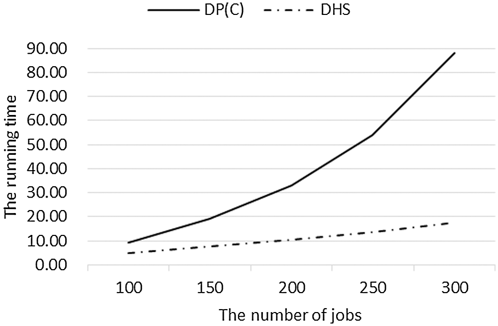
Figure 9: The average running time of DP(C) and DHS for large-scale-jobs experiments
Table 4 shows the results of the three algorithms on the relative percentage deviation under small-scale-jobs experiments and large-scale-jobs experiments.
Using the data in Table 4, we plot the relationship between the average RPD of algorithm DHS and the number of jobs in Fig. 10.
From Fig. 10, we can get that: (1) Since DP(C) and B&B are both exact algorithms, their average RPDs are 0. The average RPD of DHS is large in the small-scale-jobs case and decreases rapidly with the increase of the number of jobs, which means that the accuracy of DHS increases quickly with the rise of the number of jobs. However, in the small-scale-jobs case, the difference between the solution of DHS and the optimal solution is more than 25%, especially when the number of jobs is less than 15, the error is more than 50%; (2) In the large-scale-jobs case, with the increase of n, the reduction speed of the average RPD slows down. In all large-scale-jobs experiments, the average RPD is above 0.1. Even if n reaches 300, the gap between it and the optimal solution is still 12%.
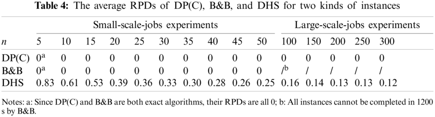
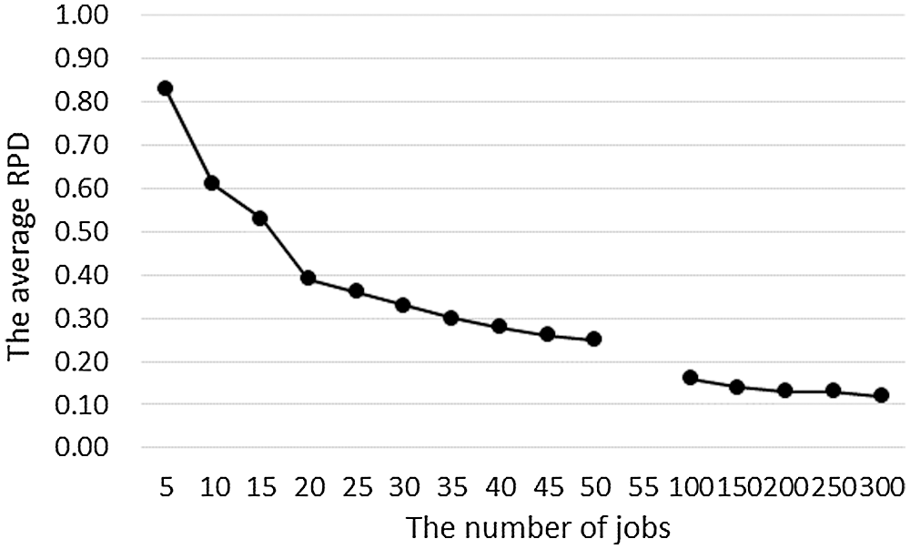
Figure 10: The average RPD of DHS changes with the number of jobs for two kinds of experiments
According to the comparative analysis of numerical experimental results in Sections 5.1 and 5.2, we can get the following results:
(1) From the perspective of algorithm time complexity, DHS has advantages, followed by DP(C). The gap between the two can be ignored in the small-scale-jobs case. Although there is a certain gap in the large-scale-jobs case, DP(C) is still within the acceptable range. B&B has significant disadvantages in running time, and when the number of jobs is greater than 45, its running time becomes unacceptable;
(2) From the perspective of algorithm accuracy, DP(C) and B&B are both exact algorithms so that they can give the optimal solution. But B&B cannot provide the optimal solution within the time limit when the number of jobs is immense. DHS is a heuristic algorithm. In the small-scale-jobs case, the accuracy is low, and the gap with the optimal solution is more than 25%. In the large-scale-jobs case, the accuracy is improved, but the gap with the optimal solution is still more than 12%;
(3) The running time of DP(C) is small, and the accuracy is better than DHS 50% in the small-scale-jobs case. Although there is a certain gap between DP(C) and DHS, the running time of DP(C) is still in the acceptable range. And the algorithm accuracy is better than DHS 12% in the large-scale-jobs case.
This paper studies two two-stage hybrid flow-shop problems with two machines and fixed processing sequences, widely used in shared manufacturing, stock control systems, and other manufacturing areas. Two objectives of minimizing makespan and total weighted completion time are considered. For these two models, we first show they are both ordinary NP-hard, present a dynamic programming algorithm for each model, and analyze the time complexity of each algorithm. Then, the relationship between the running time and the combination of the total processing time of the flexible tasks and the number of jobs is obtained by numerical experiments. Finally, the advantages and disadvantages of the dynamic programming algorithms presented in this paper are compared with the exact algorithm B&B and the heuristic algorithm DHS, which have advantages in solving hybrid flow-shop problems.
In future research, we will study the polynomial-time approximation algorithm with a smaller worst-case ratio for this problem and extend the dynamic programming algorithm's design method given in this paper to other scheduling problems with fixed processing sequences.
Acknowledgement: This work was partially supported by the Zhejiang Provincial Philosophy and Social Science Program of China (Grant No. 19NDJC093YB), the National Social Science Foundation of China (Grant No. 19BGL001), the Natural Science Foundation of Zhejiang Province of China (Grant No. LY19A010002) and the Natural Science Foundation of Ningbo of China (The design of algorithms and cost-sharing rules for scheduling problems in shared manufacturing, Acceptance No. 20211JCGY010241).
Funding Statement: This study was funded by the Zhejiang Provincial Philosophy and Social Science Program of China (Grant No. 19NDJC093YB), Recipient: Qi Wei. And the National Social Science Foundation of China (Grant No. 19BGL001), Recipient: Qi Wei. And the Natural Science Foundation of Ningbo of China (Acceptance No. 20211JCGY010241), Recipient: Qi Wei. And the Natural Science Foundation of Zhejiang Province of China (Grant No. LY19A010002), Recipient: Yong Wu.
Conflicts of Interest: The authors declare that they have no conflicts of interest to report regarding the present study.
1. Vairaktarakis, G., Lee, C. Y. (2004). Analysis of algorithms for two-stage flowshops with multi-processor task flexibility. Naval Research Logistics, 51, 44–59. DOI 10.1002/nav.10104. [Google Scholar] [CrossRef]
2. Wei, Q., He, Y. (2005). A two-stage semi-hybrid flowshop problem in graphics processing. Applied Mathematics: A Journal of Chinese Universities B, 20, 393–400. DOI 10.1007/s11766-005-0016-6. [Google Scholar] [CrossRef]
3. Zhong, W. Y., Shi, Y. (2018). Two-stage no-wait hybrid flowshop scheduling with inter-stage flexibility. Journal of Combinatorial Optimization, 35(1), 108–125. DOI 10.1007/s10878-017-0155-8. [Google Scholar] [CrossRef]
4. Li, Y., Li, X., Gao, L. (2020). Review on hybrid flow shop scheduling problems. China Mechanical Engineering, 31(23), 2798. DOI 10.3969/j.issn.1004-132X.2020.23.004. [Google Scholar] [CrossRef]
5. Lin, B. M. T., Hwang, F. J. (2011). Total completion time minimization in a 2-stage differentiation flowshop with fixed sequences per job type. Information Processing Letters, 2011, 111(5), 208–212. DOI 10.1016/j.ipl.2010.11.021. [Google Scholar] [CrossRef]
6. Yu, C., Xu, X., Yu, S., Sang, Z., Yang, C. et al. (2020). Shared manufacturing in the sharing economy: Concept, definition and service operations. Computers & Industrial Engineering, 146, 106602. DOI 10.1016/j.cie.2020.106602. [Google Scholar] [CrossRef]
7. Jiang, Y. W., Wei, Q. (2011). An improved algorithm for a hybrid flow-shop problem in graphics processing. Acta Automatica Sinica, 37(11), 1381–1386. DOI 10.3724/SP.J.1004.2011.01381. [Google Scholar] [CrossRef]
8. Wei, Q., Wu, Y. (2020). Dynamic programming algorithms for two-machine hybrid flow-shop scheduling with a given job sequence and deadline. IEEE Access, 8, 89964–89975. DOI 10.1109/ACCESS.2020.2993857. [Google Scholar] [CrossRef]
9. Zhang, M., Lan, Y., Han, X. (2020). Approximation algorithms for two-stage flexible flow shop scheduling. Journal of Combinatorial Optimization, 39(1), 1–14. DOI 10.1007/s10878-019-00449-3. [Google Scholar] [CrossRef]
10. Peng, A. Z., Liu, L. C., Lin, W. F. (2021). Improved approximation algorithms for two-stage flexible flow shop scheduling. Journal of Combinatorial Optimization, 41(1), 28–42. DOI 10.1007/s10878-020-00657-2. [Google Scholar] [CrossRef]
11. Wang, S., Kurz, M., Mason, S. J., Rashidi, E. (2019). Two-stage hybrid flow shop batching and lot streaming with variable sublots and sequence-dependent setups. International Journal of Production Research, 57(22), 6893–6907. DOI 10.1080/00207543.2019.1571251. [Google Scholar] [CrossRef]
12. Tan, Y., Monch, L., Fowler, J. W. (2017). A hybrid scheduling approach for a two-stage flexible flow shop with batch processing machines. Journal of Scheduling, 21(2), 209–226. DOI 10.1007/s10951-017-0530-4. [Google Scholar] [CrossRef]
13. Dong, J., Pan, H., Ye, C., Tong, W., Hu, J. (2020). No-wait two-stage flowshop problem with multi-task flexibility of the first machine. Information Sciences, 544, 25–38. DOI 10.1016/j.ins.2020.06.052. [Google Scholar] [CrossRef]
14. Wang, S., Wang, X., Yu, L. (2020). Two-stage no-wait hybrid flow-shop scheduling with sequence-dependent setup times. International Journal of Systems Science: Operations & Logistics, 7(3), 291–307. DOI 10.1080/23302674.2019.1575997. [Google Scholar] [CrossRef]
15. Shao, W., Shao, Z., Pi, D. (2021). Effective constructive heuristics for distributed no-wait flexible flow shop scheduling problem. Computers & Operations Research, 136, 105482. DOI 10.1016/j.cor.2021.105482. [Google Scholar] [CrossRef]
16. Feng, X., Zheng, F., Xu, Y. (2016). Robust scheduling of a two-stage hybrid flow shop with uncertain interval processing times. International Journal of Production Research, 54(12), 1–12. DOI 10.1080/00207543.2016.1162341. [Google Scholar] [CrossRef]
17. Ahonen, H., Alvarenga, A. G. (2017). Scheduling flexible flow shop with recirculation and machine sequence-dependent processing times: Formulation and solution procedures. The International Journal of Advanced Manufacturing Technology, 89(1–4), 765–777. DOI 10.1007/s00170-016-9093-3. [Google Scholar] [CrossRef]
18. Lei, D., Wang, T. (2020). Solving distributed two-stage hybrid flowshop scheduling using a shuffled frog-leaping algorithm with memeplex grouping. Engineering Optimization, 52(9), 1461–1474. DOI 10.1080/0305215X.2019.1674295. [Google Scholar] [CrossRef]
19. Cai, J., Zhou, R., Lei, D. (2020). Fuzzy distributed two-stage hybrid flow shop scheduling problem with setup time: Collaborative variable search. Journal of Intelligent & Fuzzy Systems, 38(3), 3189–3199. DOI 10.3233/JIFS-191175. [Google Scholar] [CrossRef]
20. Rolf, B., Reggelin, T., Nahhas, A., Müller, M., Lang, S. (2020). Scheduling jobs in a two-stage hybrid flow shop with a simulation-based genetic algorithm and standard dispatching rules. Winter Simulation Conference, pp. 1584–1595. Florida, USA. [Google Scholar]
21. Wang, S., Wang, X., Chu, F., Yu, J. B. (2020). An energy-efficient two-stage hybrid flow shop scheduling problem in a glass production. International Journal of Production Research, 58(8), 2283–2314. DOI 10.1080/00207543.2019.1624857. [Google Scholar] [CrossRef]
22. Shafransky, Y. M., Strusevich, V. A. (1998). The open shop scheduling problem with a given sequence of jobs on one machine. Naval Research Logistics, 45(7), 705–731. DOI 10.1002/(SICI)1520-6750(199810)45:73.0.CO;2-F. [Google Scholar] [CrossRef]
23. Hwang, F. J., Kovalyov, M. Y., Lin, B. M. T. (2012). Total completion time minimization in two-machine flow shop scheduling problems with a fixed job sequence. Discrete Optimization, 9(1), 29–39. DOI 10.1016/j.disopt.2011.11.001. [Google Scholar] [CrossRef]
24. Hwang, F. J., Kovalyov, M. Y., Lin, B. M. T. (2014). Scheduling for fabrication and assembly in a two-machine flowshop with a fixed job sequence. Annals of Operations Research, 217(1), 263–279. DOI 10.1007/s10479-014-1531-8. [Google Scholar] [CrossRef]
25. Lin, B. M. T., Hwang, F. J., Kononov, A. V. (2016). Relocation scheduling subject to fixed processing sequences. Journal of Scheduling, 19(2), 153–163. DOI 10.1007/s10951-015-0455-8. [Google Scholar] [CrossRef]
26. Halman, N., Vinetz, U. (2021). An FPTAS for two performance measures for the relocation scheduling problem subject to fixed processing sequences. Optimization Letters, 2021, 1–16. DOI 10.1007/s11590-021-01772-7. [Google Scholar] [CrossRef]
27. Cheref, A., Agnetis, A., Artigues, C., Billaut, J. C. (2017). Complexity results for an integrated single machine scheduling and outbound delivery problem with fixed sequence. Journal of Scheduling, 20(6), 681–693. DOI 10.1007/s10951-017-0540-2. [Google Scholar] [CrossRef]
28. Cheng, T. C. E., Kravchenko, S. A., Lin, B. M. T. (2019). Server scheduling on parallel dedicated machines with fixed job sequences. Naval Research Logistics, 66(4), 321–332. DOI 10.1002/nav.21846. [Google Scholar] [CrossRef]
29. Cheng, T. C. E., Kravchenko, S. A., Lin, B. M. T. (2020). Complexity of server scheduling on parallel dedicated machines subject to fixed job sequences. Journal of the Operational Research Society, 2020, 1–4. DOI 10.1080/01605682.2020.1779625. [Google Scholar] [CrossRef]
30. Ji, M., Zhang, W. Y., Liao, L. J., Cheng, T. C. E., Tan, Y. Y. (2019). Multitasking parallel-machine scheduling with machine-dependent slack due-window assignment. International Journal of Production Research, 57(6), 1667–1684. DOI 10.1080/00207543.2018.1497312. [Google Scholar] [CrossRef]
31. Moursli, O., Pochet, Y. (2000). A branch-and-bound algorithm for the hybrid flowshop. International Journal of Production Economics, 64, 113–125. DOI 10.1016/S0925-5273(99)00051-1. [Google Scholar] [CrossRef]
32. Nirmal Kumar, S. J., Ravimaran, S., Alam, M. M. (2020). An effective non-commutative encryption approach with optimized genetic algorithm for ensuring data protection in cloud computing. Computer Modeling in Engineering & Sciences, 125(2), 671–697. DOI 10.32604/cmes.2020.09361. [Google Scholar] [CrossRef]
33. Shao, W., Shao, Z., Pi, D. (2020). Modeling and multi-neighborhood iterated greedy algorithm for distributed hybrid flow shop scheduling problem. Knowledge-Based Systems, 194, 105527. DOI 10.1016/j.knosys.2020.105527. [Google Scholar] [CrossRef]
34. Pang, X., Xue, H., Tseng, M. L., Lim, M. K., Liu, K. (2020). Hybrid flow shop scheduling problems using improved fireworks algorithm for permutation. Applied Sciences, 10(3), 1174. DOI 10.3390/app10031174. [Google Scholar] [CrossRef]
35. Karaci, A., Yaprak, H., Ozkaraca, O., Demir, I., Simsek, O. (2019). Estimating the properties of ground-waste-brick mortars using DNN and ANN. Computer Modeling in Engineering & Sciences, 118(1), 207–228. DOI 10.31614/cmes.2019.04216. [Google Scholar] [CrossRef]
36. Zini, H., Elbernoussi, S. (2017). Minimizing makespan in hybrid flow shop scheduling with multiprocessor task problems using a discrete harmony search. IEEE International Conference on Computational Intelligence & Virtual Environments for Measurement Systems & Applications, pp. 177–180. Annecy, France. [Google Scholar]
37. Wang, S., Liu, M., Chu, C. (2015). A branch-and-bound algorithm for two-stage no-wait hybrid flow-shop scheduling. International Journal of Production Research, 53(4), 1143–1167. DOI 10.1080/00207543.2014.949363. [Google Scholar] [CrossRef]
38. Priya, A., Sahana, S. K. (2020). Multiprocessor scheduling based on evolutionary technique for solving permutation flow shop problem. IEEE Access, 8, 53151–53161. DOI 10.1109/ACCESS.2020.2973575. [Google Scholar] [CrossRef]
 | This work is licensed under a Creative Commons Attribution 4.0 International License, which permits unrestricted use, distribution, and reproduction in any medium, provided the original work is properly cited. |