Computer Modeling in Engineering & Sciences

DOI: 10.32604/cmes.2022.019336

ARTICLE

A High-Efficiency Inversion Method for the Material Parameters of an Alberich-Type Sound Absorption Coating Based on a Deep Learning Model

Yiping Sun1,2, Jiadui Chen1, Qiang Bai1, Xuefeng Zhao1 and Meng Tao1,*

1School of Mechanical Engineering, Guizhou University, Guiyang, 550025, China
2Aviation Academy, Guizhou Open University, Guiyang, 550023, China
*Corresponding Author: Meng Tao. Email: tomn_in@163.com
Received: 17 September 2021; Accepted: 22 November 2021

1  Introduction

A sound-absorbing coating composed of cavities in a viscoelastic material has application potential in vibration and noise reduction, sound insulation, filtering, acoustic stealth, etc. The applications of these materials in information, communication, and military are of great significance. A cavity in a viscoelastic material, such as rubber, is formed to have the basic structure of the anechoic coating. The basic shape of the cavity is a cylinder with a uniform cross section or a cone with a cross section that varies with the thickness. The main function of the cavity is to make the anechoic coating resonate in the low-frequency range to expand the effective sound absorption frequency band. The technique of laying a structure with periodically arranged cavities on a target surface to improve the acoustic performance, such as a reflective baffle or sound-absorbing cover on stealth submarines, has been widely used [1–5]. After years of development, based on the physical properties of materials and the structure of a sound-absorbing coating composed of cavities in a viscoelastic material, the use of traditional theoretical analysis and numerical calculations to carry out acoustic research has achieved prolific results [6–23].

A theoretical analysis method [6–13] can explain the sound absorption mechanism of anechoic coatings well, but the shortcomings are that it is difficult to analyse and requires high professional theoretical knowledge of the acoustic wave equation and the propagation mode of the acoustic wave in the medium. These analytical methods mainly include the one-dimensional model [6], two-dimensional theory [7], four-factor-modified bright spot model [8], transfer matrix calculation method [9–11], and a theoretical framework for acoustic wave propagation [12,13]. In terms of numerical research [14–16], the greatest advantage of the numerical calculation method is that there are no restrictions on the shape of the cavity, and the applicable conditions are wide; however, the disadvantage is that the calculation is time-consuming, and it is difficult to optimize the design. In addition, Ivansson et al. [17,18] transplanted electron scattering and optical band gap calculations into the analysis of viscoelastic sound-absorbing coatings, and the acoustic performance of anechoic coatings with periodic distributions of spherical cavities and ellipsoidal cavities was calculated. Some scholars have studied the optimal design of the acoustic performance of a sound absorbing coating composed of cavities in a viscoelastic material [19–23]. The above research shows that the study of the acoustic performance of a cavity cover has become a key research direction worldwide, and the main research methods have been concentrated on traditional numerical analysis, mechanism research, optimization design and experimental verification.

However, traditional methods are unable to manipulate sound waves accurately and effectively; and have analysis difficulties, time-consuming solution processes, and large optimization search spaces. Therefore, it is of great significance to find a research method that can quickly, efficiently and automatically generate the structure and material parameters of a sound-absorbing cover layer according to the expected acoustic performance target. In this case, a suitable design for an anechoic coating can be obtained for different needs. Currently, a data-driven artificial neural network (ANN) combined with a sound-absorbing coating composed of cavities in a viscoelastic material has advantages that traditional methods lack. For example, no feature engineering is required, which effectively overcomes the shortcomings of the difficulty of meshing in the finite element method (FEM); data-driven methods apply end-to-end learning without intermediate processes; and large amounts of information can be generated in batches, which saves time and economic costs [24–26]. ANNs have achieved world-renowned success in photoacoustic tomography, material defect detection, robot vision, natural language processing, energy prediction and other fields, and they are currently a popular research topic [27–31]. Deep learning is an important branch of ANNs, and it is interdisciplinary to study how computers simulate human learning patterns to obtain new knowledge or skills. The basic idea is to design an algorithm to determine the rules between input data and output data based on a given dataset. If the rules between the input and output are not changed, once new input data are given, their output can be automatically and quickly calculated, and the accuracy can be improved by increasing the depth of the network.

To date, deep learning has made the reasoning ability of computers a reality through dataset optimization and has shown results in acoustic performance prediction. Jeon et al. [32] performed an ANN estimation of the sound absorption coefficient of four-layer fibre materials and compared the results with those of the transfer matrix method that used multiple nonacoustic parameters to estimate the sound absorption coefficient of a multilayer film. Ciaburro et al. [33] predicted the sound absorption coefficient of electrospun polyvinylpyrrolidone/silica composites based on an ANN. Paknejad et al. [34] used an ANN, the adaptive neural-fuzzy inference system (ANFIS) and a genetic algorithm (GA) to predict the sound absorption coefficient of acrylic carpets at different frequencies, and the applicability and performance of the ANN-GA hybrid model in the prediction of carpet piles were verified. Nevertheless, although deep learning has achieved certain results in the field of acoustic research, there are still few studies on the application of the acoustic performance of cavity sound-absorbing overlays; in particular, research on the inversion of sound-absorbing coating parameters and the prediction of acoustic performance according to the expected acoustic performance targets has not yet been published. Since deep learning has natural advantages in automatically mining undefined rules [24], we associate deep learning theory with the study of a sound absorbing coating composed of cavities in a viscoelastic material and hope to design an anechoic coating's structure and material parameters according to the anticipated acoustic performance goals. In this way, it will lead to a disruptive breakthrough in the field of sound-absorbing cover layers, making the design process fast, efficient and automated. More importantly, this method does not require professional theoretical requirements for designers, and only requires attention to actual needs rather than a complicated design process.

In the case of the Alberich-type sound absorption coating, as the basis for the study of other forms of anechoic coatings, this paper proposes a reverse research method based on the combination of an autoencoder (AE) and a multilayer perceptron (MLP), called the AEMLP method, to efficiently invert the material parameters of the Alberich-type sound absorption coating. On this basis, a predictive model called the simulator was trained to rapidly predict the acoustic performance. For other anechoic coatings with different cavity forms, the parameters can also be inverted efficiently, the acoustic performance can be predicted rapidly according to the method proposed in this paper, and only the structure and material parameters need to be modified accordingly.

The method of directly generating material parameters according to the anticipated acoustic performance targets automates the design process with higher efficiency and less time consumption. It is an effective research tool, especially for lay users who do not have professional acoustic theory knowledge. The organization structure of this paper is as follows: Section 2 describes the Alberich-type sound absorption coating structure and the material parameters. The overall design idea and theoretical method of the deep learning AEMLP model are introduced. Section 3 explains the results from the aspects of data collection, the AEMLP model's training, the material parameters’ inversion testing, the acoustic performance rapid prediction method and the sound absorbers’ design. Section 4 concludes the paper with a summary of the methods presented in this paper.

2  Modelling

2.1 Features of Coating and an Introduction of AEMLP

This section mainly introduces the efficient AEMLP research method. We use the deep learning method to link the material parameter characteristics of the coating with the reflection coefficient characteristics. First, we introduce the structure and material parameter characteristics of the cell unit. Then, the overall design idea of AEMLP is introduced from the training and generation aspects of the reflection coefficient and material parameters.

2.1.1 Properties of the Cell Unit

Fig. 1 shows the reflection coefficient parameters, the cylindrical cavity acoustic coating and the cell unit. The main function of the cylindrical cavity is to make the sound-absorbing coating resonate at a lower frequency to absorb sound waves, thereby broadening the effective sound-absorbing frequency band of the coating [35].

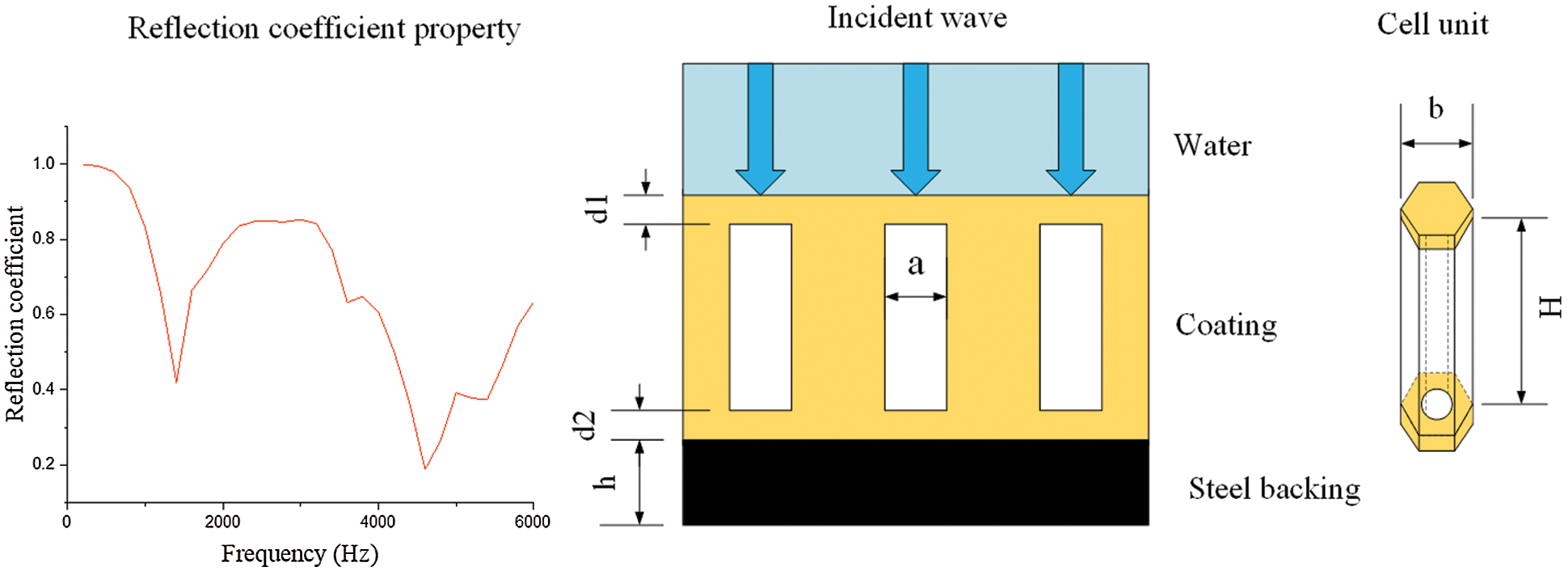
Figure 1: Schematic diagram of the acoustic performance and the covering structure

The outer diameter of the cell unit and the material parameters of the viscoelastic Alberich-type sound absorption coating are shown in Table 1; here, the regular hexagonal unit is treated as a cylindrical unit [16].

Obviously, there is a close relationship between the characteristic column vector of each material parameter and the reflection coefficient, and each column vector corresponds to a set of reflection coefficients. The rules between the reflection coefficient and the feature column vector of the material parameters can be determined with a deep learning model, and the material parameter features can be automatically inverted from the reflection coefficient. To describe the design principle more clearly, based on the FEM, we performed a parametric scan of the 4704 feature column vectors to calculate the reflection coefficient of the viscoelastic Alberich-type sound absorption coating by using COMSOL Multiphysics 5.6. According to the literatures [16,36–39] on the acoustic performance of a sound absorbing coating composed of cavities in a viscoelastic material, the consistency of the comparison results of the reflection coefficient is shown in Fig. 2, which proved that the result of using the FEM to solve the reflection coefficient is credible.

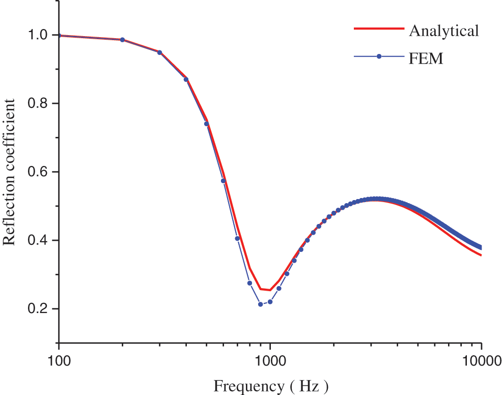
Figure 2: Comparison of the analytical and numerical solutions

2.1.2 Composition of AEMLP

To obtain an AEMLP deep learning model, we used the normalized material parameters of the Alberich-type sound absorption coating in matrix X as the reconstruction data and the reflection coefficient matrix Y as the input data of the MLP. The training process of AEMLP includes data collection, feature extraction, data reconstruction and feature matching, as shown in Fig. 3. Specifically, first, the material parameters of the layer are processed into a matrix X by the maximum-minimum method, the feature extraction method of the encoder is used to map X into a 30-dimensional latent space, and a matrix of material parameters is reconstructed by applying the decoder. Then, the reflection coefficient Y of the FEM is used as the input data of the MLP, the features of Y are extracted to match the latent space, and a fully connected MLP is used as a deep learning algorithm to make the matching more effective and easier to implement.

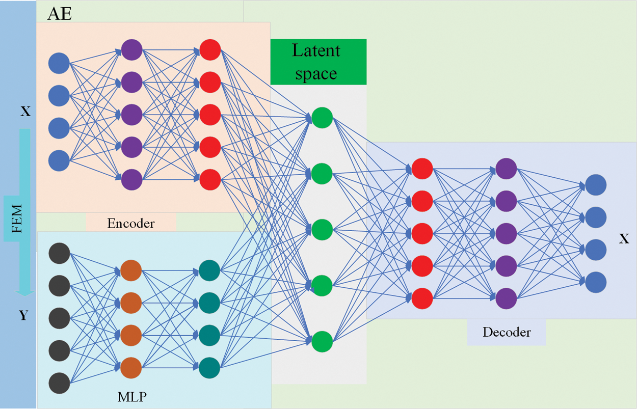
Figure 3: The composition of the AEMLP model

2.2 Theory of AEMLP

This section mainly describes the technical details of the training process for the AEMLP model. The training process can be divided into three parts: material parameter preprocessing, feature extraction and data reconstruction, and feature matching. In terms of material parameter preprocessing, we used the maximum-minimum method to normalize the parameters. During feature extraction, an AE-based method was used to map the material parameters into a latent feature space with 30 dimensions and reconstruct them. To match the reflection coefficient with the mapped latent feature space, we use a fully connected neural network with an MLP to obtain connections.

2.2.1 Pre-Processing of Inputs

Since the inputs include the density, elastic modulus, loss factor and Poisson's ratio of the coating and have different measurement units and value ranges, normalization preprocessing of the inputs is critical to the success of the model. We used the maximum-minimum normalization preprocessing method in Eq. (1) [40].

Xscaled=X−XminXmax−Xmin(1)

where X is the input feature parameter vector, Xminis the minimum value vector of the input feature parameters, Xmax is the maximum value vector of the input feature parameters, and Xscale of the input feature parameters ranges from 0 to 1 and is dimensionless. This normalized preprocessing method makes different input parameters comparable even if they belong to different value ranges or are expressed in different measurement units, as shown in Fig. 4.

Figure 4: Normalization method of material parameters

2.2.2 Feature Extraction and Data Reconstruction

The next step after the normalization of the material parameters is to use the AE deep learning method to extract features. We established an AE model, which is an ANN composed of two parts: the encoder function z = f(x) and the decoder function x = g(z). The output dimension of the encoder is 30 to facilitate feature matching with the output values of the MLP, and the decoder is used to reconstruct the input data. The process of material parameter feature extraction and data reconstruction based on AE is shown in Fig. 5.

Figure 5: Flow chart of AE feature extraction and data reconstruction

Our main purpose is to map the material parameters into the latent feature space and retain the data of the space by the encoder while recording the decoder part of the AE model. The main component of the AE model is called a fully connected ANN, and information is forwarded through the network layer. The propagation process is as Eq. (2).

M=σn(⋅⋅⋅⋅⋅⋅σ2(σ1(Xw1+b1)w2+b2)⋅⋅⋅⋅⋅⋅+bn)(2)

where X is a column vector, which represents the feature vector composed of the extracted acoustic cover layer's density, elastic modulus, loss factor and Poisson's ratio. w is the weight matrix connecting the activation value of the previous layer of neurons and the current layer of neurons, and b is the bias. M is the feature vector mapped from the activation function of the last layer, and it is the material parameter vector of the coating reconstructed by the decoder. After the model is established, the vector X containing the normalized material parameters is input into the network, and the reconstructed material parameters are generated by updating the weight matrix w and the bias b. The mean square error loss function is used to measure the difference between the predicted value and the true value. Here, we use the loss estimation parameters of backpropagation; to be precise, for the last layer of the network, the process of minimizing the loss function can be defined as Eq. (3).

minLoss(w,b|M,O)=12∑n = 1N(M−O)2(3)

where M is the predicted value, which is calculated from the activation function of the last layer and O is the label value of the material parameters corresponding to the input sample features.

In back propagation, a gradient descent algorithm is used to update the weight matrix and bias to minimize the loss function. According to the backpropagation principle, the loss function gradient of the output layer is Eq. (4).

∇wjnLoss=σ′⋅(Mn−On)⋅OjL - 1(4)

For a given training set, the label value of On is a constant. In actual training, we initialize the bias b to 0 and only need to update the weights to minimize the loss function during backpropagation. Therefore, the loss function depends only on the weight coefficient w. Our goal is to make the loss function as small as possible. According to the backpropagation algorithm, we obtain the update formula of wjn as Eq. (5).

wjn←wjn+Δwjn=wjn−η⋅∇wjnLoss(5)

where η is the learning rate; the larger η is, the faster wjn is updated.

2.2.3 Feature Matching

In terms of deep learning methods, for the MLP network, the inputs are the feature vectors of the reflection coefficient. Since the latent feature space and the reflection coefficient are matched through the last layer of the MLP, the accuracy of the matching has been effectively improved. When the features match, the loss function is defined as Eq. (6).

Loss(w,b|Q,Z)=12∑n = 1N(Q−Z)2(6)

where Q is the output matrix after the reflection coefficient is propagated through the MLP and Z is the latent feature space. w and b denote the weights and biases of the MLP model; here, N = 30.

From the point of view of digital signals, for our task, the target output range is from 0 to 1. Therefore, we choose the sigmoid function as the activation function of the last layer, which is defined as Eq. (7).

σ=11+e−x(7)

The sigmoid function can handle any output from 0 to 1; specifically, for a larger negative input, the output is 0, and for a larger positive input, the output is 1. The derivative of the sigmoid is easy to calculate. Using the sigmoid activation function, the final output can be strictly limited between 0 and 1 according to the goal we set. The process of feature matching is shown in Fig. 6.

Figure 6: Feature matching process

In addition, to solve the overfitting problem, we introduce a dropout layer into the model. This is a technique to avoid overfitting in training, which randomly stops the coefficients in the hidden layer, thereby avoiding the dependence of coefficient updates on the connection effect of fixed hidden nodes.

3  Parameter Inversion and Sound Absorber Design

3.1 Dataset

AEMLP is a supervised deep learning model that requires a dataset containing the material parameters of the Alberich-type sound absorption coating and the corresponding reflection coefficients, where the material parameters are used as the label values of the dataset. Here, we use the cell unit structure shown in Fig. 1. The cell unit structure and material parameters determine the reflection coefficient of the layer. According to Section 2.1.1, 4704 sets of material parameter vectors are generated by uniform sampling, and then these material parameter vectors are put into COMSOL Multiphysics, and periodic conditions are applied to the cell boundary to calculate the reflection coefficient. Table 2 shows the distribution of the detailed dataset, where the reflection coefficients are the inputs of the MLP, and the material parameters are used as the input data of AE and need to be reconstructed. To be precise, 90% of the data are set as the training set and the remaining 10% are used as the test set; therefore, there are 4234 sets of training samples and 470 sets of test samples. It should be pointed out that 48 sets of test samples were specified in the 470 sets of test samples, and these 48 sets included 7 sets of duplicate samples; hence, 41 sets of test samples were specified sampled. Since the input features are 4-dimensional data, we adopted the distributed stochastic neighbour embedding (t-SNE) [41] method to visualize them by using dimensionality reduction. Fig. 7 shows the distribution of the input features after dimensionality reduction. The purpose of specifying the test data is to facilitate observation, and the distribution of the test set still maintains the characteristics of random sampling. Generally, in terms of the amount of training data for deep learning, we are more concerned about the ratio of the number of samples to the number of features rather than just the number of samples. For our task, we hope to fit 30-dimensional features with 4234 sets of samples, and the ratio of the number of samples to the number of features is 141.13, which is sufficient from the perspective of theoretical analysis [42].

Figure 7: Distribution of the inputs. X1 and X2 are the two dimensions after dimension reduction

3.2 Model Training and Testing

The AEMLP model is established in a Windows 10 operating system. The computer configuration is an Intel(R) Core (TM) i5–8265U CPU @ 1.6 GHz/8 GB/512 G SSD. The deep learning algorithm is implemented on the Anaconda platform with Python version 3.7, and the model is built using TensorFlow 2.0 and the Keras framework.

3.2.1 Model Training

The detailed training process of the AEMLP method is shown in Fig. 8. We first applied maximum-minimum normalization to the matrix of the material parameters and randomly divided it. Then, we used AE to extract the features of the material parameters and reconstructed them. The training parameters are batch = 100, learning rate = 0.001, and epoch = 300. The activation function of the hidden layers is the rectified linear unit (ReLU) function, which effectively avoids gradient dispersion and gradient explosion. The activation function of the last layer is the sigmoid function, which ensures that the output range is from 0 to 1. The selected optimizer is adaptive moment estimation (Adam) with momentum. It should be pointed out that by comparing the Euclidean distance between the input feature matrix of material parameters and the output feature matrix of AE reconstruction, the accuracy of the AE reconstruction result is 99.86%.

Figure 8: Flow chart of AEMLP training

3.2.2 Testing

First, we define the ability in which a slight change in material parameters does not change the acoustic performance of the coating as “material robustness”. Therefore, the greater the influence of material parameters on the acoustic performance is, the weaker the material robustness; in contrast, the smaller the influence of the material parameters on the acoustic performance is, the stronger the material robustness. Obviously, when the material parameters are inverted, the smaller the error is, the weaker the material robustness, and the larger the error is, the stronger the material robustness. There are 48 sets of material parameters sampled in the test set, and the result of the inversion using AEMLP is shown in Fig. 9.

Figure 9: Inversion results of the material parameters (a) inversion result of density (b) inversion result of modulus (c) inversion result of loss factor (d) inversion result of Poission's ratio

In Fig. 9a, the inverted density is basically consistent with the change trend of the label value and fluctuates near the label value, which indicates that the density is of good material robustness. The reason is that the density affects the amplitude of the reflection coefficient, and when the deep learning algorithm performs logistic regression on the density, the value of the loss function is not zero, which leads to density fluctuations.

Fig. 9b shows the inversion result of the elastic modulus. The smaller the elastic modulus is, the smaller the inversion error, and the larger the elastic modulus is, the greater the inversion error, which means that the greater the elastic modulus is, the stronger the material robustness. This is because as the modulus of elasticity increases, the material becomes harder and the phase velocity becomes larger, which will eventually cause a serious mismatch between the impedance of the covering layer and the water; hence, the sound wave cannot effectively enter the covering layer in this situation. After the impedance mismatch, the effect of increasing the elastic modulus on the acoustic performance of the coating becomes weak.

Fig. 9c shows the inversion result of the loss factor. Except for the extremely large error at point 47, in general, the smaller the loss factor is, the smaller the inversion error, and the larger the loss factor is, the greater the inversion error, which indicates that a larger loss factor implies more material robustness. This is because when the increase in the loss factor reaches a certain point, the sound wave becomes attenuated in the coating, and even if the loss factor continues to increase, it will not change the acoustic performance of the coating, especially after the lowest-order wave is attenuated.

Fig. 9d shows the inversion result of Poisson's ratio. When the elastic modulus is small, the inversion error is generally small for all Poisson's ratio values. When the elastic modulus is large, the following properties hold: the smaller Poisson's ratio is, the larger the inversion error, and the larger Poisson's ratio is, the smaller the inversion error. This indicates that when the elastic modulus is small, for all Poisson's ratio values, the material robustness is weak. When the elastic modulus is large, the following properties hold: the smaller Poisson's ratio is, the greater the material robustness, and the larger Poisson's ratio is, the less the material robustness. In other words, when the elastic modulus is small, Poisson's ratio has a greater impact on the acoustic performance, and when the elastic modulus is large, a larger Poisson's ratio affects the acoustic performance of the coating.

Fig. 10 shows the accuracy results when the AEMLP method is applied to invert the material parameters of the test set. We compared some classic machine learning methods, such as decision tree, random forest, ridge regression and K-nearest neighbour (KNN) methods [43–46]. It can be clearly seen that AEMLP is superior to these classic machine learning methods and has an average accuracy rate of 95.03%. In practical applications, the deep learning model only predicts the probability, and its accuracy cannot reach 100%; therefore, further optimization of the network's depth, number of neurons and hyperparameters is required. Even so, the value calculated by deep learning is close to the label value, which can reduce the amount of calculation and speed up the design process. The research results thus far show that the AEMLP model proposed in this paper can accurately and effectively invert the material parameters of the Alberich-type sound absorption coating.

Figure 10: Accuracy comparison of AEMLP and other classic machine learning algorithms

3.3 Rapid Prediction of Acoustic Performance

3.3.1 Prediction Model

The FEM is often very time-consuming when it is used to determine the acoustic performance of a coating, and the experimental measurement of the reflection coefficient is very expensive. For these reasons, based on the AEMLP model, we trained a simulator model to directly obtain the reflection coefficients corresponding to the inverted material parameters. In this way, the shortcomings of time-consuming FEM and expensive experimental measurements were solved. The design process is shown in Fig. 11. The simulator is an MLP model, and the appendix illustrates its network structure and working principle. Taking the expected reflection coefficient as the acoustic performance target, the simulator model combined with AEMLP can efficiently invert the material parameters and rapidly predict their acoustic performance. For the inverted material parameters of the 48 sets of test data in Fig. 9 in Section 3.2.2, the reflection coefficients predicted by the simulator and the simulation results of the FEM are shown in Figs. 12–14.

Figure 11: Simulator and AEMLP combination to rapidly predict the acoustic performance

Fig. 12 shows the predicted reflection coefficients of the inverted material parameters under the conditions that the difference between the loss factor and Poisson's ratio is small and the density and elastic modulus are different. The results predicted by the simulator are basically the same as the results obtained by the FEM. Only when the modulus of elasticity is very small at high frequencies above 4000 Hz will there be a small error, as shown by the red and blue stippled lines in Figs. 12a11–12a41; this small error is caused by the predictive characteristics of the simulator model when the modulus of elasticity is small. Nevertheless, the error is within the acceptable range, indicating that under this condition, the simulator prediction method is effective.

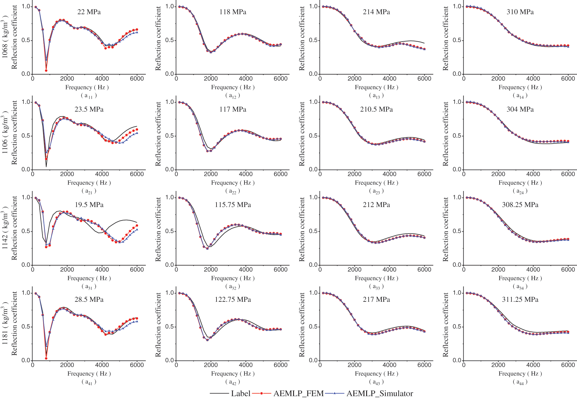
Figure 12: Sound reflection coefficient values of the (a11–a14) 22 MPa, 118 MPa, 214 MPa, and 310 MPa modulus samples with a 1068 kg/m­3 density, 0.325 loss factor, and 0.476 Poisson's ratio; (a21–a24) 23.5 MPa, 117 MPa, 210.5 MPa, and 310 MPa modulus samples with a 1106 kg/m­3 density, 0.349 loss factor, and 0.4732 Poisson's ratio; (a31–a34) 19.5 MPa, 115.75 MPa, 212 MPa, and 308.25 MPa modulus samples with a 1142 kg/m­3 density, 0.3844 loss factor, and 0.4706 Poisson's ratio; (a41–a44) 28.5 MPa, 122.75 MPa, 217 MPa, and 311.25 MPa modulus samples with a 1181 kg/m­3 density, 0.3228 loss factor, and 0.4692 Poisson's ratio

In general, under different density conditions, the reflection coefficient predicted by the simulator model does not change with the peak and trough frequencies of the label value, and the change trend is basically the same, as shown by the black line and blue stippled line in Fig. 12. Among them, the difference between the black line and the blue stippled line in Figs. 12a11–12a41 shows that when the elastic modulus is small, there is a certain difference in the amplitude of the trough. Furthermore, the density affects the amplitude of the reflection coefficient, which is consistent with the result in Fig. 9a. Furthermore, there is a certain error between the predicted reflection coefficient and the label value at high frequencies above 4000 Hz, which is due to the weaker material robustness when the AEMLP method is inverted with a smaller elastic modulus, which is consistent with the result in Fig. 9b. In addition, the high frequency above 4400 Hz in Fig. 12a13 and the frequency above 3000 Hz in Fig. 12a31 have large errors, indicating that the accuracy of the AEMLP method is not 100%, which is consistent with the results in Fig. 10.

Fig. 13 shows the reflection coefficient predicted from the inversion results of the material parameters when the elastic modulus and loss factor are different under the same density and Poisson's ratio values. Only when the elastic modulus and loss factor are small and the reflection coefficient predicted by the simulator is at a high frequency above 4000 Hz will there be a certain error in the result obtained by the FEM, as shown in Fig. 13a11 by the red and blue stippled lines, which is caused by the predictive characteristics of the simulator model under a small elastic modulus and loss factor. Nevertheless, the predicted reflection coefficient curve is basically consistent with the change trend of the FEM, indicating that the simulator prediction method is effective under this condition.

Figure 13: Sound reflection coefficient values when the density is 1068 kg/m­3, Poisson's ratio is 0.476, and the loss factor samples are 0.09, 0.325, 0.56, and 0.795 for moduli of (a11–a14) 22 MPa, (a21–a24) 118 MPa, (a31–a34) 214 MPa, and (a41–a44) 310 MPa, respectively

When the elastic modulus is constant, the smaller the loss factor is, the larger the error between the label value and the inversion result, as shown by the black and blue stippled lines in Figs. 13a11–13a14 and 13a21–13a24. This is due to the poor material robustness of the AEMLP method in the inversion of smaller loss factors, which corresponds to the result in Fig. 9c. When the loss factor is constant, the smaller the elastic modulus, the larger the error between the reflection coefficient predicted by the inversion result and the label value is, as shown by the black line and blue stippled line in Figs. 13a11–13a41. This is due to the weaker material robustness in the inversion of the smaller elastic modulus by AEMLP, which further verifies the result in Fig. 9b.

Fig. 14 shows the predicted reflection coefficients from the inversion results when the elastic modulus and Poisson's ratio are different under the same density and loss factor conditions. The results predicted by the simulator are highly consistent with those of the FEM, and only when the modulus of elasticity is small do the trough values of their reflection coefficients have slight differences; therefore, the error can be ignored, as shown in Figs. 14a11 and 14a14 by the red and blue stippled lines. This shows that the simulator prediction method is effective under this condition.

Figure 14: Sound reflection coefficient values when the density is 1181 kg/m­3, the loss factor is 0.3844, and Poisson's ratio values are 0.4706, 0.47884, 0.48708, and 0.49532 for moduli of (a11–a14) 38.75 MPa, (a21–a24) 115.75 MPa, (a31–a34) 212 MPa, and (a41–a44) 308.25 MPa, respectively

When the elastic modulus is small, the predicted reflection coefficient and the label value have a certain error, as shown in Figs. 14a11–14a14 with the black line and the blue stippled line. The reason is that when the elastic modulus is small, Poisson's ratio has a greater impact on the acoustic performance. Under this condition, AEMLP has a weak material robustness to changes in Poisson's ratio; in contrast, when the elastic modulus is large, a large Poisson's ratio value will have an impact on the acoustic performance. Therefore, the error between the predicted reflection coefficient and the label value becomes large in this situation, as shown in Figs. 14a34 and 14a43 by the black line and blue stippled line. The result is consistent with the result in Fig. 9d.

By analysing the results of Fig. 9 and from Figs. 12–14, the following conclusions can be drawn: It is effective to invert material parameters and predict the reflection coefficient with the combined simulator and AEMLP model.

To further illustrate the advantages of the simulator more intuitively, we compared it with the FEM in terms of computational time consumption and the number of degrees of freedom to be solved, as shown in Fig. 15. The times required for the simulator and FEM to obtain a single reflection coefficient target are 3 s and 238 s, respectively. The simulator is nearly 80 times faster than the FEM. It is worth noting that the simulator has good batch processing capabilities, and there is no need to increase the time consumption when performing batch calculations. For example, the calculation time required by the simulator to solve the reflection coefficient in batches for the above 48 sets of test data is still 3 s, while the FEM needs to parameterize the test data one by one, which takes a total of 14,912 s. Moreover, because the simulator is an end-to-end deep learning model, the number of iterations is only one, and the FEM needs to iteratively solve 34,966 degrees of freedom; hence, the simulator model further improves the prediction efficiency when predicting multiple acoustic targets. The simulator's batch processing and end-to-end learning capabilities make the simulator prediction method more efficient and reduce the difficulty of the design.

Figure 15: Time consumption and calculation iteration comparisons of the simulator and FEM

3.3.2 Design of the Sound Absorber

As an example, to obtain the desired low-frequency, broadband, strong attenuation properties and effectively manipulate sound waves, we designed a sound absorber with optimal sound absorption performance and a three-band absorber of an Alberich-type sound absorption coating.

First, to obtain the low-frequency, wide-band, and strong attenuation characteristics required by the Alberich-type sound absorption coating, we refer to the literature [35] and use the fitting method to initially set the expected sound absorption coefficient, as shown in Fig. 16a. It should be noted that a certain fitting error is allowed when initially setting the sound absorption coefficient; subsequently, we use Eq. (8) to solve the expected reflection coefficient corresponding to the optimal sound absorber, as shown in Fig. 16b.

α=1−R2(8)

The reflection coefficient R is input into the AEMLP model, and the inverted material parameters are shown in Table 2. Other than the inverted elastic modulus, which is 20 MPa larger than the average value in the literature [35], the other parameters are basically consistent with those in the literature. The reason why the inverted elastic modulus is slightly larger is that there is a certain fitting error in the sound absorption coefficient that we initially set.

Then, we applied the simulator model to predict the actual reflection coefficient and calculated the sound absorption coefficient, as shown in Figs. 16c and 16d, respectively. From the comparison in Fig. 16, it can be seen that the predicted amplitudes and frequencies of the peak and trough of the sound absorption coefficient and reflection coefficient are basically equal to the expected values, and the trends of the curves are basically the same, which means that the method is effective for the inversion of the material parameters of the Alberich-type optimal sound absorber. It should be noted that the average of the predicted sound absorption coefficient of the Alberich-type optimal sound absorber above 1000 Hz is 0.81, which is 0.05 lower than the average sound absorption coefficient in the literature [35], in which only the material parameters were optimized; this is mainly because the Alberich-type sound absorption coating that we use has a cylindrical cavity structure, while the coating in the literature [35] has a structure with cylindrical and truncated cone cavities, where the composition cavity improves the sound absorption performance of the coating. On the other hand, the literature considers the dynamic characteristics of the material parameters, and we simplify the material parameters to constants and ignore the influence of frequency on the material parameters, which also causes the average sound absorption coefficient of the designed optimal sound absorber to be slightly smaller.

Figure 16: Optimal sound absorber: (a) expected sound absorption coefficient, (b) expected reflection coefficient, (c) comparison of sound absorption coefficients, and (d) comparison of reflection coefficients

The above inversion results of an optimal absorber on the material parameters of the Alberich-type sound absorption coating with the best sound absorption performance illustrate the effectiveness of the method in this paper. On this basis, to better explain how to effectively manipulate sound waves, we set the sound absorption coefficient of the coating with the expected three-band sound absorption performance, as shown in Fig. 17a. The corresponding reflection coefficient is shown in Fig. 17b. When the frequencies are 800 Hz, 2600 Hz and 4800 Hz, the amplitudes of the absorption coefficient of the three-band sound absorber are set as 0.85, 0.8 and 0.99, respectively. The inversion results of the material parameters are shown in Table 3.

Figure 17: The three-band sound absorber: (a) expected sound absorption coefficient, (b) expected reflection coefficient, (c) comparison of sound absorption coefficients, and (d) comparison of reflection coefficients

The comparison of the acoustic performance predicted by the material parameters of the three-band sound absorber using the simulator and the FEM are shown in Figs. 17c and 17d, respectively.

Due to the small elastic modulus and loss factor of the three-band sound absorber, a certain deviation was in the amplitudes of the peaks and troughs, as shown in Figs. 17c and 17d by the red dotted line and blue short dashed-dot line, which are related to the characteristics of the simulator prediction model. They are consistent with the result in Fig. 13a11. The reason for the error is that the simulator prediction model is a logistic regression model, and its predicted results cannot reach 100% accuracy.

Although there is a certain deviation between the black solid line and blue short dashed-dotted line in Figs. 17c and 17d, both the peak frequency of sound absorption from the low to middle frequencies and the sound absorption peak value at the high frequencies are generally the same. This shows that the AEMLP deep learning-based model successfully inverted the material parameters of the anechoic coating.

Obviously, through the above two examples, it is shown that the method proposed in this paper achieves the low-frequency, broadband, and strong attenuation design goals and effectively manipulates sound waves. Therefore, it is effective to use the method proposed in this paper to invert the material parameters of an Alberich-type sound absorption coating for the expected acoustic performance targets.

4  Conclusion

This paper first proposes the AEMLP research method to invert material parameters based on the acoustic performance of an Alberich-type sound absorption coating. Once the acoustic performance design goals of the coating are input into the trained deep learning model, the corresponding material parameters are automatically generated, and the accuracy of the inversion result of the material parameters is as high as 95.03%. Subsequently, we introduce a simulator method based on AEMLP, which addresses the time-consuming shortcomings of the FEM. As examples, we used the AEMLP method to invert the material parameters of an Alberich-type sound absorption coating for an optimal sound absorption coefficient and three-band sound absorption performance. The consistency between the acoustic performance of the optimal sound absorber and the design goal proves the effectiveness of the method; however, the deviation in the three-band sound absorber from the design target indicates that the AEMLP model has the disadvantage of insufficient generalization because the AEMLP model only considers the inversion of material parameters with a cylindrical cavity structure and a fixed scale. To further enhance the model's reverse design capability and accurately manipulate sound waves in a larger range, the next step will be to enrich the cavity structure and expand size parameters on the basis of existing work.

Compared with traditional methods, in the study of the acoustic performance of Alberich-type sound absorption coatings, the AEMLP method is superior to the general methods in terms of the number of calculation iterations, design time consumption, and result accuracy. Moreover, the efficiency is significantly improved, the design process is accelerated, the calculation and human resources are significantly reduced, and the trained model can be applied to new functions with different acoustic performance goals without additional training. Theoretically, the inversion of the material parameters of different structures can be realized by only completing the transformation of the dataset. In addition, the AEMLP method requires less professional knowledge in the field of acoustic wave theory and acoustic materials, and the material parameters can be automatically generated on demand. It provides an effective design tool for engineering and technical personnel, especially lay users. Users only need to focus on the expected acoustic performance design goals, rather than researching optimal design theory for optimization search calculations.

Acknowledgement: We would like to thank Cunhong Yin and other members of the materials team for helpful discussions. We are grateful for the support of the Doctoral Workstation of Guizhou Open University. We thank the developers of TensorFlow 2.0, which we used for all our experiments.

Availability of Dataset: The dataset and code for this article can be found online at https://github.com/sunyiping1987/AEMLP_SIMULATOR.git.

Appendix: Supporting information on the simulator model is available from the author.

Funding Statement: This work was supported by the National Natural Science Foundation of China (Nos. 51765008, 11304050); the High-Level Innovative Talents Project of Guizhou Province (No. 20164033); the Science and Technology Project of Guizhou Province (No. 2020–1Z048); and the Open Project of the Key Laboratory of Modern Manufacturing Technology of the Ministry of Education (No. XDKFJJ [2016] 10).

Conflicts of Interest: The authors declare that they have no known competing financial interests or personal relationships that could have appeared to influence the work reported in this paper.

This work is licensed under a Creative Commons Attribution 4.0 International License, which permits unrestricted use, distribution, and reproduction in any medium, provided the original work is properly cited.