Computer Modeling in Engineering & Sciences

DOI: 10.32604/cmes.2022.019855

ARTICLE

Modeling and Analyzing for a Novel Continuum Model Considering Self-Stabilizing Control on Curved Road with Slope

Li Lei1, Zihao Wang2,* and Yong Wu3

1School of Energy and Power Engineering, Shandong University, Jinan, 250061, China
2School of Control Science and Engineering, Shandong University, Jinan, 250061, China
3Department of Logistics Management, Ningbo University of Finance and Economics, Ningbo, 315175, China
*Corresponding Author: Zihao Wang. Email: wangzihao621@mail.sdu.edu.cn
Received: 20 October 2021; Accepted: 12 November 2021

1  Introduction

The accelerated development of modern intelligent transportation system not only alleviates traffic congestion, but also improves the stability of the transportation system [1–5]. However, the stability of traffic system is also easily affected by various driver characteristics, such as self-stabilizing, memory, backward-looking, and road geometry (e.g., slope and curved road). Therefore, it is a critical and urgent task to improve the stability of traffic flow by fully considering the driver characteristics and road geometry.

Generally speaking, there are three types of traffic models: microscopic models [6–12], lattice models [13–20], and macroscopic hydrodynamic models [21–27]. The macro model mainly refers to the continuous medium model of traffic flow, which regards a large number of vehicles as compressible continuous medium and studies the comprehensive average behavior of the vehicle group. This type of model tries to characterize the traffic flow with the average density ρ, average speed v, and flow q and study the functional relationship it satisfies. As early as 70 years ago, Lighthill et al. [28,29] first proposed the continuous medium model of traffic flow. Later in 1956, Richards [30] independently proposed the LWR model, which is analogous with continuum model. According to the basic idea of car-following theory, the motion equation (i.e., acceleration equation) is introduced into the continuous medium model to form a high-order continuous medium model of traffic flow mechanics [31]. Whihtma established a similar model, so the model is often called Pyane-Whihtam (PW) model [32].

Traffic flow theory has been the focus of scientific research since it was put forward. Countless scientific and technological workers have devoted a lot of effort to exploration and research. Jiang et al. [33] proposed a full velocity difference model (FVDM) considering the positive and negative speed difference comprehensively. Zhang et al. proposed a macroscopic model considering the speed difference between adjacent vehicles on the slope [34]. Sun et al. developed an extended micro model is proposed considering the driver's desire for smooth driving on a curved road [35]. Gong et al. [36] designed a hybrid system and simulated human driving and autonomous vehicles. By using Gamma-convergence, it is proved that the optimal control problem of the mean-field can be solved at the microscopic level. Peng et al. analyzed the impact of self-stabilization on traffic stability considering the current lattice's historic flux for a two-lane freeway [37]. Although these papers attempt to use simulation platforms to develop vehicle dynamics models, they did not connect driver characteristics with geometric characteristics of the road. Therefore, this study attempts to bridge this critical defect.

The paper is organized as follows: Section 2 proposes a new continuum model considering the effect of self-stabilizing is constructed on the curved road with slope. Sections 3 and 4 present the linear and nonlinear analysis, and then the neutral stability curve and the KdV equation describing the nonlinear density wave are obtained. Section 5 carries out numerical experiments that demonstrate how the stability of traffic flow is affected by self-stabilizing, curved and slopes. Finally, the concludes are provided in Section 6.

2  The Extended Continuum Traffic Flow Model

In 2001, Jiang et al. [33] proposed the FVDM to solve the problem of vehicle retrogression based on previous studies. The model equation is

dvn(t)dt=a[V(Δxn(t))−vn(t)]+λΔvn,(1)

where the headway and velocity difference between two adjacent vehicles are Δxn=xn+1−xn and Δvn=vn+1−vn; a denotes driver's distance sensitivity coefficient; λ is the sensitivity coefficient of driver to speed difference; V(Δxn(t)) is optimal velocity function.

Based on the FVD model, Li et al. [38] proposed a new car-following model. They considered the impact of the driver's desire and the self-stabilizing control on traffic flow stability, and the extended model can be expressed as

d2xn(t)dt2=a[Vop(Δyn(t))−vn(t)]+λ1[V(h)−(1+p)vn(t−τ)]+λ2[vn(t)−(1+p)vn(t−τ)],(2)

where yn(t)=Δxn(t) is the headway difference between two adjacent vehicles; h is the average space headway distance on the straight road; V(h)−vn(t−τ) is the driver's desire for smooth driving; vn(h)−vn(t−τ) is the self-stabilizing control effect in the difference between the current and history velocity; λ1 and λ2 denote the reaction coefficients of two introduced factors, respectively; p is the reaction coefficient reflecting the uncertainty of vehicle's speed; Vop(Δyn(t)) is desired optimal velocity of vehicle n.

For the sake of avoiding more fuel caused by frequent changes in driving speed during driving, drivers can hope to drive more smoothly. On account of the FVDM, Sun et al. [35] proposed a new car-following model of curve road and considered the impact of driver's desire on traffic flow stability, and the extended model can be expressed as

d2sn(t)dt2=a[V(Δsn(t))−dsn(t)t]+λ1dΔsn(t)dt+λ2[rω(s)−rωn(t−τ)],(3)

where Δsn(t)=sn+1(t)−sn(t) is the headway between the vehicle n and vehicle n+1 on the curve road; τ is the history time; rω(s)−rωn(t−τ) represents the drive's desire for smooth driving.

Zhou et al. [39] consider a situation such that vehicles are running on a single-lane gradient highway under a periodic boundary condition, which is described in Fig. 1. Fig. 1 shows the gravitational force acts upon vehicles on the slope of the gradient.

Figure 1: Vehicles move on a gradient highway: uphill and downhill situation: uphill − and downhill +

Kaur et al. [40] make full use of road geometry to study driver's anticipation effect and further presented a new lattice model as follows:

{∂tρj+ρ0sin⁡ϕj(ρjvj−ρj−1vj−1)=γ|ρ02V′(ρ0,θ)|sin2⁡ϕj(ρj+1−2ρj+ρj−1)ρj(t+τ)vj(t+τ)=ρ0sin⁡ϕjV(ρj+1(t+ατ),θ),(4)

V(ρj(t),θ)=κμgR1cos⁡θ∓sin⁡θ2V0(ρj(t),θ),(5)

V0(ρj(t),θ)=[tanh⁡(2ρ−ρj(t)ρ02−1ρc)+tanh⁡(1ρc)],(6)

ρc(θ)=1hc(θ)=1h(1∓sin⁡θ),(7)

where κ(0<κ≤1) is control parameter; R1 is the radius of curvature, θ is slope; ϕj represents the angle for the curved road at jth site; hc(θ) is the necessary distance between two cars to avoid collision on the slope road; μ and g mean the friction coefficient and gravitational acceleration, respectively.

Through research on driver characteristics and control signals, the stability of traffic flow can be improved to a certain extent under certain conditions. However, road geometric characteristics also affect the stability of traffic flow, allowing of no to neglect. Distinguished with traditional studies, a modified car-following model on a single-lane gradient highway with curved is proposed with the consideration of the self-stabilizing effect as follows:

dωn(t)dt=ar[V(rΔαn(t))−rωn(t)]+λ[ωn(t)−ωn(t−τ)],(8)

where ωn(t) is the angular velocity of car nth at time t; α and r represent the radius and radian of the curved road.

The highlight of our proposed model is to study the influence of self-stabilizing control and curved road with the slope on traffic flow stability from a macro perspective. Here, we can convert the micro variables in Eq. (8) into macro variables through the method proposed by Liu et al. [41], as follows:

{rΔαn(t)→h(s,t)≈1ρ(s,t)−ρx2ρ3−ρxx6ρ4ωn(t)→ω(s,t)ωn(t−τ)→ω(s−ωt,t−τ)V(rΔαn(t))→(κμgrcos⁡θ∓sin⁡θ2)V0(rΔαn(t))=(κμgrcos⁡θ∓sin⁡θ2)Ve(ρ),(9)

where ρ(s,t) and ω(s,t) are macroscopic density and velocity on the curved with slope, respectively; Ve(ρ) is the equilibrium velocity and V¯′(h)=−ρ2Ve′(ρ).

For simplification, we carry out time first-order Taylor expansion for ω(s−ωτ,t−τ) while ignoring the non-linear terms, i.e.,

ω(s−ωτ,t−τ)=ω(s,t)−τdω(s,t)dt.(10)

Substituting macro variables into Eq. (8), we derive

∂ω∂t+ω∂ω∂s=ar(1−λτ)[(κμgrcos⁡θ∓sin⁡θ2)Ve(ρ)−rω].(11)

3  Linear Stability Analysis

In the literature, the theory of fluid dynamics is used to describe the traffic flow state, and its continuity fluid dynamics equation is established to study [42,43]. By combining the above formula with the continuous conservative equation, we have

{∂ρ∂t+∂(ρω)∂t=0∂ω∂t+ω∂ω∂s=ar(1−λτ)[(κμgrcos⁡θ∓sin⁡θ2)Ve(ρ)−rω].(12)

The equations are rewritten into matrices to simplify the analysis as follows:

∂U∂t+A∂U∂s=E,(13)

where

{U=[ρω]A=[ωρ0ω]E=[0ar(1−λτ)[(κμgrcos⁡θ∓sin⁡θ2)Ve(ρ)−rω]].(14)

According to Eq. (14), it is obvious that the average velocity ω is equal to the characteristic velocity λ1 and λ2, which proves that the model satisfies the characteristics of traffic flow anisotropy.

Slight interference caused by driver behavior characteristics or external factors will spread upward with the traffic flow, and the traffic-free flow will develop into congestion flow gradually. If the slight disorder tends to be stable or disappear, the traffic flow can run smoothly, therefore controlling traffic congestion. Assuming that the traffic system is a homogeneous flow at the initial time, constants ρ0 and ω0 represent the initial density and speed in the uniform state. Therefore, the steady-state solution of the uniform flow is

ρ(s,t)=ρ0,ω(s,t)=ω0.(15)

(ρ(s,t)ω(s,t))=(ρ0ω0)+(ρ^kω^k)exp⁡(iks+σkt).(16)

By substituting Eq. (16) into Eq. (12) and neglecting the nonlinear higher-order terms, we obtain the following equation:

{(σk+ω0ik)ρ^k+ρ0ikω^k=0ω^kσk+ikω0ω^k=ar(1−λτ)⋅(κμgrcos⁡θ∓sin⁡θ2)⋅(V′e(ρ0)ρ^k−rω^k)+ar(1−λτ)(ρ^kik2ρ0+ρ^k(ik)26ρ02)V′e(ρ0).(17)

The necessary and sufficient condition for the stability of linear systems is that the determinant of matrix coefficients returns to zero, i.e.,

|σk+ω0ikρ0ikar(1−λτ)⋅(κμgrcos⁡θ∓sin⁡θ2)⋅(1+ik2ρ0+(ik)26ρ0)V′e(ρ0)−[σk+ω0ik+ar(1−λτ)]|=0.(18)

Regarding ρ^k and ω^k as the unknown parameters in the equations, then we can get that σk satisfies the following quadratic equation:

(σk+ω0ik)2+(σk+ω0ik)ar(1−λτ)+ar(1−λτ)⋅κμgrcos⁡θ∓sin⁡θ2⋅ρ0Ve′(ρ0)ik(1+ik2ρ0+(ik)26ρ0)=0.(19)

According to the criterion of control theory, the neutral stable condition for the traffic flow is obtained

a=−r(1−λτ)(κμgrcos⁡θ∓sin⁡θ)ρ02Ve′(ρ0).(20)

Performing the Taylor expansion for σk as follows:

Im(σk)≈−a[ω0+ρ0κμgrcos⁡θ∓sin⁡θ2V′e(ρ0)]+o(k3).(21)

According to Eq. (21), we infer that

c(ρ0)=ω0+ρ0κμgrcos⁡θ∓sin⁡θ2Ve′(ρ0),(22)

This is similar to the velocity gradient model [44] and modified model.

The neutral stability lines for different slopes of the gradient road are plotted in Fig. 2. The neutral stability curves for uphill and downhill situations on the road, respectively, as shown in the illustration. In Fig. 2a, the stability region becomes more significant and more prominent with the addition of slope θ on the uphill slope. In contract, in Fig. 2b, in the downhill situations the stable area becomes larger and larger with the decrease of the slope.

Figure 2: Neutral stability lines for different slopes in two situations: patterns (a) and (b) are corresponding to uphill and downhill situations respectively

4  Nonlinear Analysis

For the sake of explore the nonlinear analysis of the new model, we adopt a new coordinate system as follows [33]:

z=s−ct.(23)

By substituting Eq. (23) into (12), we obtain the following equation:

{−cρz+qz=0−cωz+ω⋅ωz=ar(1−λτ)[(κμgrcos⁡θ∓sin⁡θ2)Ve(ρ)−rω]+ar(1−λτ)⋅V′e(ρ)(ρz2ρ+ρzz6ρ2).(24)

Here, traffic flow is defined as the product of density and velocity of traffic flow as q=ρωr, which can be obtained from Eq. (23):

ωz=cρzρr−qρzrρ2.(25)

Applying second-order Taylor expansion to q=ρωr yields

q=ρVe(ρ)+b1ρz+b2ρzz.(26)

Substituting the Eq. (25) into the second row of Eq. (12), it can be written as

−c(cρzρr−qρzrρ2)+qρ(cρzρr−qρzrρ2)=ar(1−λτ)[(κμgrcos⁡θ∓sin⁡θ2)Ve(ρ)−qρ]+ar(1−λτ)⋅V′e(ρ)(ρz2ρ+ρzz6ρ2)(κμgrcos⁡θ∓sin⁡θ2).(27)

The coefficients b1 and b2 are determined by balancing the terms ρz and ρzz in Eq. (27), so we get

{b1=(1−λτ)a(c−Ve(ρ))2+V′e(ρ)2(κμgrcos⁡θ∓sin⁡θ4)b2=16ρ(κμgrcos⁡θ∓sin⁡θ2)V′e(ρ).(28)

Eq. (26) can be rewritten with Taylor expansions near the neutral stability condition

ρVe(ρ)≈ρhVe(ρh)+(ρVe)ρ|ρ=ρhρ^+12(ρVe)ρρ|ρ=ρhρ^2.(29)

Substituting the Eq. (24) into Eq. (29), and turning the ρ^ to ρ, we obtain the following equation:

−cρz+[(ρVe)ρ+(ρVe)ρρρ]ρz+b1ρzz+b2ρzzz=0.(30)

Aiming at obtaining the standard KdV-Burgers equation, we perform the following transformations:

U=−[(ρVe)ρ+(ρVe)ρρρ],X=mx,T=−mt.(31)

Considering Eq. (24), the KdV-Burgers equation is obtained as follows:

UT+UUX−mb1UXX−m2b2UXXX=0.(32)

One analytical solution of the above KdV-Burgers equation is

U=−3(−mb1)225(−m2b2)[1+2tanh⁡(±−mb110m2)(X+6(−mb1)225(−m2b2)T+ζ0)+tanh2(±−mb110m2)(X+6(−mb1)225(−m2b2)T+ζ0)],(33)

in which ζ0 is an arbitrary constant.

5  Numerical Simulation

This section presents simulation studies to illustrate the effect of self-stabilizing of our developed dynamic model on a single-lane highway with slope. According to the time forward difference and space centre difference, the space and time are divided into space step Δx and time step Δt, for numerical simulation

ρij+1=ρij+ΔtΔxρij(ωij−ωi+1j)+ΔtΔxωij(ρi−1j−ρij).(34)

ωij+1=ωij−ΔtΔxωijr(1−λτ)(ωij−ωi−1j)+aΔtr(1−λτ)[(κμgrcos⁡θ∓sin⁡θ2)Ve(ρij)−rωij]+aΔtr(1−λτ)[ρi+1j−ρij2ρijΔx+ρi+1j−2ρij+ρi−1j6(ρij)2(Δx)2]V′e(ρij),(35)

where ρij and ωij represent density and speed on the condition of (i,j), and the space and time section are represented by i and j, respectively.

5.1 Shock Waves and Rarefaction Waves

Traffic wave is a kind of nonlinear wave, which can evolve into so-called “traffic shock” as time goes on. Therefore, we study the influence of small disturbance on the spatiotemporal evolution of density and velocity under crowding and sparsity. The Riemann initial conditions are considered as follows:

ρup1=0.04veh/m,ρdown1=0.18veh/m(36)

ρup2=0.18veh/m,ρdown2=0.04veh/m(37)

where ρup1,2 and ρdown1,2 are the density of upstream and downstream, respectively. The corresponding initial speeds are expressed as follows:

vup1,2=Ve(ρup1,2),vdown1,2=Ve(ρdown1,2).(38)

Then, we adopted equilibrium velocity function by Castillo et al. [45] as follows:

Ve=vf[1−exp⁡(1−exp⁡(nmvf(ρmρ−1)))],(39)

where ρm is the density of vehicle under congestion flow; vf and nm respectively denote free flow speed and the propagation speed of density wave under congestion density. Thus, we can obtain the evolution of Eqs. (36)--(39) (see Figs. 3 and 4). The propagation of shock-wave and rarefaction-wave patterns can be smooth and backward in Figs. 3 and 4. As time goes on, the resulting rarefaction wave disturbance propagates in the negative direction of x and is not amplified, which further validates that our proposed model satisfies the anisotropy.

Figure 3: The shock wave in the initial Riemann condition (36): (a) time-space evolution of density and (b) time-space evolution of speed

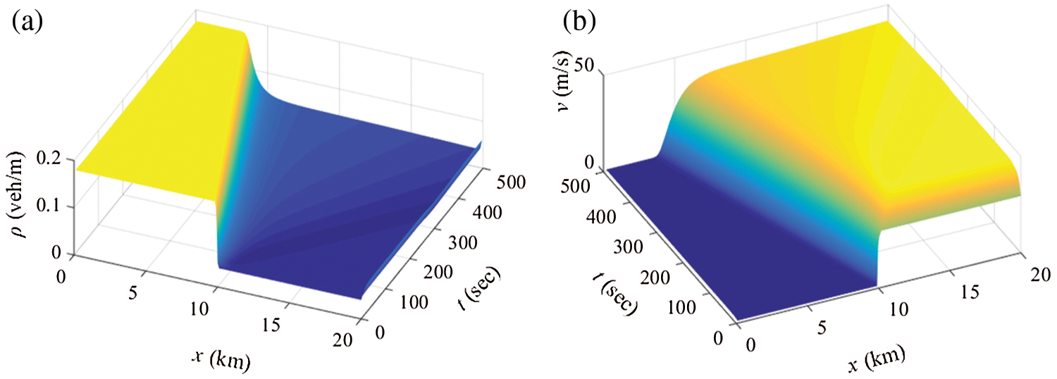
Figure 4: The rarefaction wave in the initial Riemann condition (37): (a) time-space evolution of density and (b) time-space evolution of speed

5.2 Local Cluster Effect

In this section, for clarity, we will verify the effects of self-stabilizing control strategy and different slopes and radius by conducting numerical simulation. The traditional method of stability simulation is to check the anti-disturbance ability of homogeneous traffic flow. In the literature [46], the average density ρ0 has a generalized form as follows:

ρ(s,0)=ρ0+Δρ0{cosh−2[160L(s−5L16)]−14cosh−2[40L(s−11L32)]},(40)

where the road length L=32.2km and Δρ0 is density perturbation. We adopt the periodic boundary conditions as follows:

ρ(L,t)=ρ(0,t),v(L,t)=v(0,t).(41)

Based on Kerner et al. [47], we introduce the equilibrium speed-density relationship as follows:

Ve(ρ)=vf[(1+exp⁡ρ/ρm−0.250.06)−1−3.72×10−6].(42)

First of all, Fig. 5 is the nonlinear density wave of traffic flow with self-stabilizing control in the proposed macro traffic model on the uphill and downhill slope with curved roads. Figs. 5a–5c are the uphill angle, when the road slope is sight, the influence of minor disturbance on the stability of traffic flow will not be amplified. However, Figs. 5e–5g are the downhill angle, with the increase of slope angle, the impact of disruption is more and more prominent, and the traffic flow is more unstable. Therefore, with the change of a time, there will be time stop effect or traffic flow cluster effect.

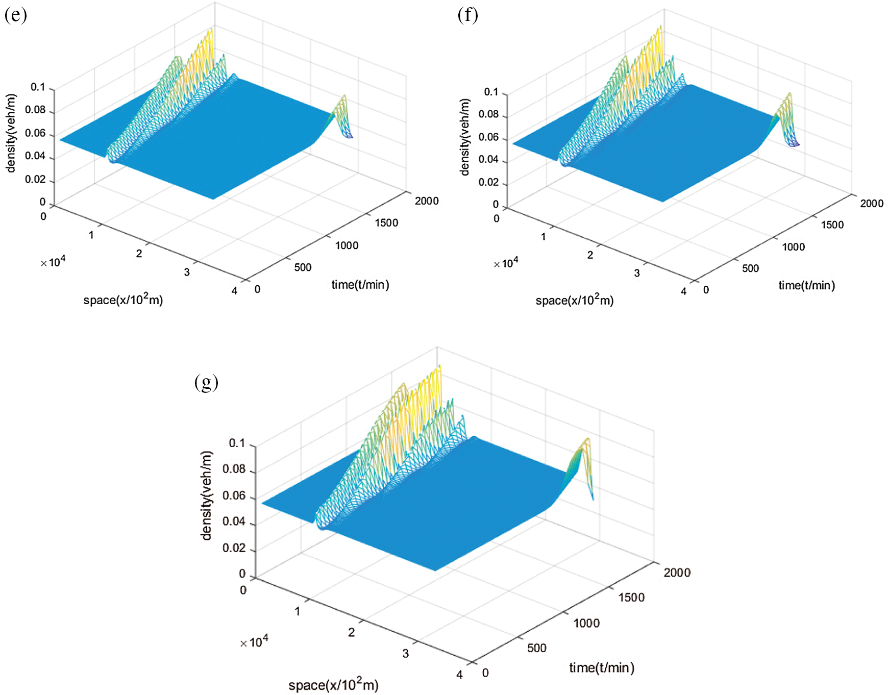
Figure 5: The evolution of the temporal and spatial on a downhill scenario with different θ when ρ0=0.055veh/m, r=20m, λ=0.6. (a)θ=6∘(b)θ=4∘(c)θ=2∘(d)θ=0∘(e)θ=2∘(f)θ=4∘(g)θ=6o

To explore the second case of road geometric characteristics: the influence of curve on traffic flow, our numerical simulation is shown in Fig. 6. It shows the evolution of traffic flow density with different curved road radii. Numerical simulation shows that when other conditions remain unchanged, the radius is large, the centripetal force is large, and the traffic flow is more unstable. It can be proved that the larger curve radius has a negative influence on the traffic stability.

Next, we explore the effect of self-stabilizing control strategy on traffic flow stability as Fig. 7. It shows that with the increasing control coefficient, the nonlinear density wave of traffic flow becomes more stable, which indicates that the stop and go phenomenon gradually disappears. Numerical simulation results illustrate that the effect of self-stability is helpful to improve the stability of traffic flow.

Figure 6: Space-time evolution of the headway for different radius r=20m,40m,60m,80m when ρ0=0.055veh/m, λ=0.6, θ=2∘(Downhill). (a)r=20m(b)r=40m(c)r=60m(d)r=80m

Figure 7: Space-time evolution of the headway for different λ values when ρ0=0.055veh/m, r=20m, θ=2∘(Downhill). (a)λ=0.2(b)λ=0.4(c)λ=0.6(d)λ=0.8

6  Conclusion

This paper introduces the effect of self-stabilizing control strategy and road geometric characteristics on traffic flow stability from a macro perspective. According to the maximum limit of the actual road slopes, different slope θ=0∘,2∘,4∘,6∘, and different radius r=20,40,60,80m are set. At the same time, the control strategy is obtained by using the historical speed and the current speed difference of the considered vehicles. We prove that the proposed traffic flow macro model guarantees the anisotropic characteristics. Under certain conditions, the model is analyzed theoretically, including linear and nonlinear stability analysis. Through Matlab simulation, the new model can accurately simulate traffic flow phenomena such as shock-wave and rarefaction-wave. The numerical simulation clearly verifies that the self-stabilizing strategy can effectively resist the influence of disturbance on the traffic flow and reduce the immense traffic pressure in the traffic flow. Road characteristic is also closely related to the stability of traffic flow, which is consistent with the theoretical study in this paper.

Funding Statement: This work is supported by the Natural Science Foundation of Zhejiang Province, China (Grant No. LY19A010002).

Conflicts of Interest: We declare that we have no financial and personal relationships with other people or organizations that can inappropriately influence our work, there is no professional or other personal interest of any nature or kind in any product, service and/or company that could be construed as influencing the position presented in the manuscript entitled “Modeling and analyzing for a novel continuum model considering self-stabilizing control on curved road with slope”.

This work is licensed under a Creative Commons Attribution 4.0 International License, which permits unrestricted use, distribution, and reproduction in any medium, provided the original work is properly cited.