| Computer Modeling in Engineering & Sciences |
DOI: 10.32604/cmes.2022.018867
ARTICLE
Partitioning of Water Distribution Network into District Metered Areas Using Existing Valves
1Department of Civil Engineering, Visvesvaraya National Institute of Technology, Nagpur, 440010, India
2Department of Civil and Architectural Engineering, Aarhus University, Aarhus, 8000, Denmark
*Corresponding Author: Neeraj Dhanraj Bokde. Email: neerajdhanraj@cae.au.dk
Received: 21 August 2021; Accepted: 11 November 2021
Abstract: Water distribution network (WDN) leakage management has received increased attention in recent years. One of the most successful leakage-control strategies is to divide the network into District Metered Areas (DMAs). As a multi-staged technique, the generation of DMAs is a difficult task in design and implementation (i.e., clustering, sectorization, and performance evaluation). Previous studies on DMAs implementation did not consider the potential use of existing valves in achieving the objective. In this work, a methodology is proposed for detecting clusters and reducing the cost of additional valves and DMA sectorization by considering existing valves as much as possible. The procedure of DMAs identification has been divided into three stages, i.e., a) clusters identification; b) sectorization or boundaries optimization and c) performance evaluation of the partitioned network. The proposed methodology is evaluated on a simple network and a real-world water network with the findings provided and compared to the DMAs, established for a raw water network with no existing valves. It is found that there is an adequate difference in cost of strategy implementation in both the cases for the network under consideration and the existing valve system achieved better network performance in terms of resilience index.
Keywords: Clusters identification; district metered areas; existing valves; sectorization; water distribution networks
Water utilities are bound to operate WDNs with adequate pressure and supply good quality water at all times. The operation of a network is a task with multiple objectives to be considered. The expanding urban infrastructure leads to new settlements and as a consequence, the size of WDNs increases and adds to the complexity in the management and operation of existing water networks. Water loss is a common problem for the water utility system and a nuisance to the management [1]. There are various strategies for controlling the leakages like pressure management through optimal localization of pressure reducing valves [2] or by partitioning the WDNs into District Metered Areas (DMAs) (or zones used alternatively in this study). The concept of partitioning the WDNs into zones was introduced to address the problem of leakage reduction. The boundaries of such zones are defined and optimized such that hydraulic parameters are within the desired range.
Each WDN is unique based on its size and topology, and so is the process of DMAs formation. The design of DMAs involves the closure of certain boundary pipes which break down the looped nature of WDNs, affecting the reliability and redundancy of the network. Apart from this, the permanent closure of a few boundary pipes leads to an increased number of dead ends and consequent deterioration of water quality. Another important aspect of the DMA design is the total cost, which involves installation costs of flow meters, isolation valves at boundary pipes, and in some cases pressure control valves at DMA inlets.
The implementation of DMAs not only eases the operation and maintenance of the network but also helps to achieve ambitious goals such as addressing the leakage problems, pressure management, and contaminant detection and control [3]. However, as the looped nature of WDNs is broken due to the closure of certain boundary pipes, the reliability and redundancy of the network is affected. Therefore, for establishing the DMAs, a trade-off between the positive and negative aspects need to be managed adequately.
The important factors that affect the DMAs design includes: (a) Size of DMAs; (b) identification of main lines (or trunk mains) and; (c) nature of boundaries (static or dynamic), etc. These are discussed as follows:
a) Size of DMAs: The size of a DMA indicates the number of customers to be served per DMA. It is related to the accuracy of the detectable leak, i.e., the smaller the DMA size, the smaller is the leak size that can be identified. The IWA guidelines recommend a DMA size of 500–5,000 properties [4]. Sizing the DMA based on a fixed number of customers is subjective, as the cost of implementation of DMAs is not accounted for. An optimal DMA size should be determined based on a thorough analysis of data relevant to the network under consideration and the financial capability of water utilities.
b) Identification of main lines: The ‘main lines’ are a series of continuously connected pipes that convey water from the source to the whole WDN. Ferrari et al. [5] suggested that the diameter of main lines should not exceed 300 mm. Perelman et al. [6] identified main lines as a connected subset of pipes having diameter and flow values greater than 400 mm and top 1% of network flow values, respectively. Ciaponi et al. [7] mentioned that a proper division could be 5%–10% main lines (with a diameter threshold of 300–500 mm as main lines) and a 90%–95% distribution network. Zhang et al. [8] proposed that the main pipes should include pipes near the natural and administrative divisions. The pipes near these boundaries lying approximately parallel can be selected as main pipes to achieve predefined or expected boundaries of the sectors.
c) Nature of boundaries: Two different considerations are identified from the literature for the DMA formation. These are: (1) DMAs with permanent boundaries; and (2) DMAs with flexible boundaries. The permanent boundary approach efficiently solved the problems of leakage reduction and establishing pressure uniformity in WDNs [9]. However, DMAs with permanent boundaries present some disadvantages like reduced resilience, deterioration of water quality [10], and occurrence of dead ends near closed pipes. In case of bursts or any other type of failure, manual valve operations are required to overcome the emergency conditions, and hence such a reactive operational approach does not provide immediate and effective incident management. Therefore, the concept of flexible DMA boundaries has emerged as an alternative [11].
DMAs design consists of clustering phase, sectorization phase, and performance evaluation of partitioned network. The general flow diagram of the procedure is shown in Fig. 1.

Figure 1: Generalized flow diagram of DMAs identification procedure
Clustering refers to the initial division of the WDN, i.e., identification of connected nodes possessing near similar features like demand, pressure, elevation, etc. A variety of algorithms are available like graph theory algorithms (Breadth first search-BFS, Depth first search-DFS, Dijkstra’s algorithm-DA, etc.) [12,13], communities’ identification algorithm (Fast Greedy Algorithm–FNA) [7,14–17], multi-agent approaches, segments identification methods [3], etc. Alvisi et al. [12] used the BFS algorithm to identify a group of nodes consisting of customer connections not exceeding 2000 numbers in each DMA. This method identified the clusters for small-sized networks and was not much suitable for large networks as it involved several iterations for identifying the appropriate size of DMAs.
di Nardo et al. [13] suggested a method of identifying clusters using the DFS algorithm. The algorithm starts from the source node and explores the network as far as possible along each path until there are no more unvisited nodes. This method was exclusively designed for multi-source networks. Diao et al. [15] were the first to use the concepts of communities’ identification, i.e., FNA for identification of clusters in water networks, however, the authors did not assign any pipe weights and treated the network as unweighted graphs. Ciaponi et al. [7] extended the work by blending the number of customers per DMA criterion (500–5000 customers) with FNA. Scarpa et al. [18] used BFS and Dijkstra’s algorithm for identifying the influence zone of each source to identify DMAs in a given multi-source water network.
Zhang et al. [9] used nodal pressure as pipe weights in communities’ identification to get pressure zones with near similar pressure in each community. Yao et al. [16] modified the convergence mechanism of FNA to improve the water demand similarity among the DMAs. Giustolisi et al. [19] integrated the concepts of segment identification with modularity function to identify the optimal segment (zone) configurations for DMA establishment. Although these algorithms can form clusters, they are sensitive to pipe weights. The clustering phase results in tentative clusters whose boundaries are finalized in the sectorization phase. It is recommended to refer to Bui et al. [20] for detailed information on clustering algorithms.
In the sectorization phase, a large number of alternative solutions may be possible, many of them may not be hydraulically feasible. For identifying the near-optimal solution, boundary pipes are optimized for their open/closed status with suitable objectives like economic criteria [21,22], pressure uniformity, leakage reduction, water age reduction, consumption reduction, reduction in unsupplied customer demand, new burst frequency reduction, contaminant control, etc., with a mandatory constraint of nodal head requirements at all times.
DMA establishment studies are multi-objective and preferred over a single objective strategy as a variety of solutions are explored, resulting in more realistic decisions. A variety of mathematical optimization and heuristic optimization tools have been used by various researchers including Linear Programming (LP) [6], Genetic Algorithm (GA) [13], Simulated Annealing (SA) [21], and Agent Swarm Optimization (ASO) [23], etc. Such algorithms require a significant amount of computational time. The computational complexity of the optimization model is of high concern, especially for heuristic methodologies [10,16,24,25] to find near-optimal solutions. Along with the development of heuristic methodologies, many-objective optimization tools swarm intelligence algorithms (like multi-objective agent swarm optimization) and evolutionary algorithms (like NSGA-II, NSGA-III, BORG algorithm) are also catching the attention [23,26,27].
di Nardo et al. [13] used a single-objective genetic algorithm to optimize the boundaries of DMAs such that the dissipated power should be minimum. Giustolisi et al. [19] used a multi- objective genetic algorithm for minimizing the leakages, unsupplied customer demand, and the number of flow meters required. Gomes et al. [21] optimized the number and location of entry points and boundary valves, along with pipe reinforcement/replacement using simulated annealing technique with pipe velocity and nodal pressure constraints. Campbell et al. [23] simultaneously optimized five objectives including economic criteria, operating criteria, and energy criteria using agent swarm optimization. Hajebi et al. [26] used many objective genetic algorithms to optimize three categories of objectives (total 13 objectives) covering structural, hydraulic, and economic criteria subjected to hydraulic, structural, and explicit bound constraints. Zhang et al. [9] used the BORG algorithm to simultaneously optimize three objectives, i.e., optimize pressure uniformity, water age uniformity, and the number of boundary pipes in a partitioned network. Recently, Liu et al. [27] suggested a multi-staged, many-objective optimization methodology for DMAs identification. The first step was to identify the tree structure of the network using minimum spanning tree algorithm [28] and the second step used many objective optimization tool (BORG) to optimize structural and hydraulic objectives simultaneously.
It has been observed from the literature that each new methodology proposed adds up a new set of partitioning parameters and hydraulic constraints. The best example of this issue is given in Hajebi et al. [26] where 13 objectives and 11 constraints were listed for DMAs identification. Simultaneous handling of such parameters or many objectives only increases computational complexity and it may exhaust the practical applicability of the methodology from the perspective of network operations. Hajebi et al. [26] methodology required 16 h to solve the BWSN-II network while the methodology of Zhang et al. [9] required 278 h for the same network with different objectives. The time complexity increases with the size of the network. Since multi-objective optimization models end up with multiple solutions for DMAs identification, multi-criteria decision-making tools such as Analytical and Hierarchical Process (AHP), TOPSIS, etc. have been used in recent studies [15,29,30].
The last step in DMA formation is the performance evaluation of a partitioned network. The performance evaluation is done to check if, each formed DMA fulfills the demands with adequate pressure heads at each node. A variety of performance indices like energy indices [31], entropy indices [14], pressure indices, fire protection indices, water quality indices [9,18], and mechanical indices can be used to evaluate the network performance after partitioning. The resilience index and water age index are the most widely used performance indicators [20]. To get detailed information on performance indices readers can refer to di Nardo et al. [32].
Even though plenty of automated methodologies are available in the literature, there are still some areas that need to be addressed. Despite multiple benefits, DMAs are rarely used for leakage control and pressure management in developing countries due to the high cost of strategy implementation.
Recently, Santonastaso et al. [33] proposed a method to adjust the water network partitioning algorithms based on topological matrices in such a way that the actual valves can be used to identify DMAs. Three different algorithms, i.e., normalized cut (NC), multilevel recursive bisection algorithm (MLRB) and edge betweenness community algorithm (EBC) were used for explicative purposes. They concluded that considering the present isolation valves is advantageous in terms of partitioning cost. Although the authors mentioned that the proposed framework tend to have slightly worse performance in terms of uniformity of nodes between DMAs and of supplied power to users, but the solutions obtained were feasible without installing additional isolation valves. It is observed that most of the approaches do not take into account, the existing valves (isolation and pressure regulating), and water meters which can significantly reduce the cost of DMAs formation. In India and several other developing countries, flow and pressure control is also achieved through valve throttling. Thus, sluice valves are provided for both isolations and flow control purposes. In real water networks, some parts of the network may face pressure deficient conditions or may have lower operational pressures. Customer satisfaction is of prime importance in any water supply scheme; hence the demand shortfall or unsupplied customer demand should be given attention while forming DMAs.
This study, therefore, addresses the problem of DMAs design using existing infrastructure to identify clusters and their boundaries. The boundaries optimization is carried out using GA with customer satisfaction as a constraint to identify permanent boundaries, followed by the performance evaluation of the obtained solution. The study proposed here is problem-specific, adapted to the problem at hand, and takes full advantage of the particularities of the problem. The procedure has been demonstrated against a small sample network and a real-life sub-zone of a water network situated in the city of Nagpur, India.
Valves are available in any existing network and normal sluice valves are used due to economic reasons for flow control and head dissipation by valve throttling. These are provided at strategic locations to serve the purpose of flow/pressure control. The same types of valves are used for isolating any section during repairs. As there is no distinction between the valves provided for two different purposes, the purpose for which they are provided could be understood from the valve opening during operation [34]. While isolation valves are fully open, flow/pressure control valves are partially open. What is required in this case is to select and combine the formed segments by these existing valves to form DMAs with no or minimum additional valves.
This section presents a methodology for defining the DMAs based on existing valve systems in a WDN using the concept of valve-to-valve segment identification. The idea here is not to create a coincidence between DMAs and segments but to identify the possible use of existing infrastructure for DMAs identification.
2.1 Segment Identification in WDN Using Existing Valves in the System
In the present study, the method proposed by Kaldenbach et al. [35] with modifications suggested by Gupta et al. [36] has been used for segments (or zones) identification using existing isolation valves.
The method considers valves as nodes in the network model and uses their exact location in segment identification using the Breadth First Search (BFS) algorithm. The basic idea of this algorithm is to automatically identify neighboring nodes of a starting node proceeding in a spoke like fashion [37]. This concept has been used to identify DMAs in water networks [12].
Such segments may not be uniform in size. Depending upon the number of connections in each segment, two or more segments can be merged based on engineering rationale to have more uniform segments. The step-by-step methodology has been explained with a small network example and also implemented on a medium-size network in the next section.
Consider the case of a small network consisting of 1 source, 15 nodes, 6 valves, and 25 links (as shown in the following Fig. 2).

Figure 2: Sample network (left) and identified segments (right). (a) Simple network (b) Valve based clusters configuration
Node-Node connectivity matrix: The first step is to form the node-node connectivity matrix. It is a square and symmetric matrix where each row and column represent a node. The nodes in the matrix have been arranged as: sources first, then junction or demand nodes, and lastly valves. If any two nodes say, node, i, and j are connected then the element in the connectivity matrix is filled up with the index number of the pipe connecting the two nodes. Table 1 shows the node connectivity matrix for the sample network.
As shown in Table 1, the matrix is divided into four quadrants, i.e., source-source/source-node/node-node connections in Quadrant I, source-valve or node-valve connections in Quadrants II and III, and valve-valve connections in Quadrant IV, respectively.
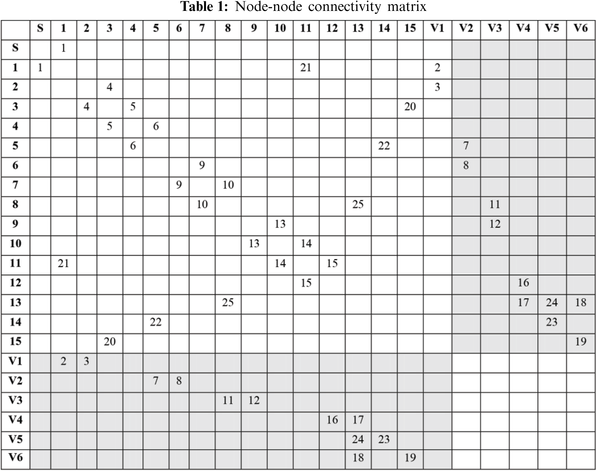
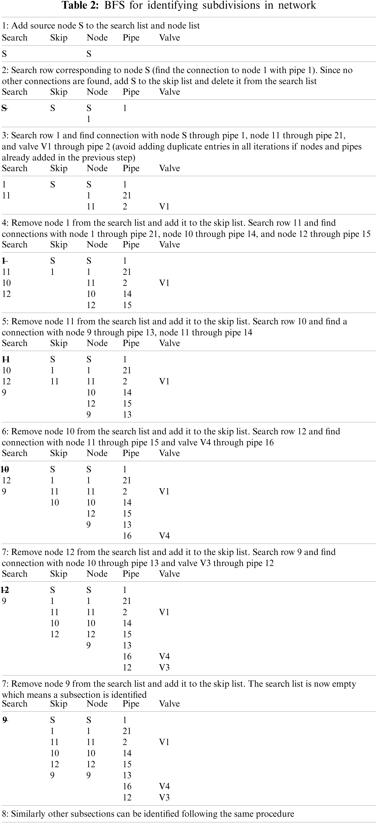
BFS for segments identification: To traverse along the network using breadth first search algorithm, various lists (or arrays) have been defined; search list (list of nodes that will be searched for connections with current segment), skip list (list of nodes that have been already searched for all segments), segment’s nodes list, segment pipes list and valves list. The following steps are performed iteratively till all the segments in the networks are identified.
(A) Add ‘first’ node to the search list and segment’s node list. Search for connections (if any) in that node’s row in Quadrant I of the connectivity matrix.
(B) If connections are found, add all the connecting nodes to the search list and segment’s node list. Check for the search list and the skip list to avoid repetitive entries of the same node.
(C) Remove the ‘first’ node from the search list and add it to the skip list.
(D) Repeat the procedure for the next node in the search list till the search list is emptied.
Once the nodes in each segment are identified, the node-node connectivity matrix is traversed again to identify the corresponding pipes and valves in the segment. The row of each node in the segment is searched using Quadrants I and II. If a connection is found in Quadrant I, it is added to the pipes list, or else, if the connection is found in Quadrant II, it is added in the valves list. It should be noted that when the connections are identified, the pipes list and the valves list are checked to avoid duplication of entries.
Lastly, single pipe segments (pipe isolated between two valves) are identified by searching the upper diagonal part of Quadrant IV as it is square and symmetrical. If such connections are found, the row value and column value are added to the new segment’s valve list and pipe list. The stepwise procedure to identify segments in the sample network is shown in Table 2.
2.2 Boundaries Optimization (Sectorization Phase)
The next step corresponds to the selection of boundary pipe status i.e., to decide which boundary pipes need to be closed or kept open to establishing permanent zones. It is a well-known fact that pressure reduction in the network due to pipe closure is proportional to the number of such ‘closed’ boundary pipes. However, when a potential boundary pipe is kept open, a flow meter must be installed on it. Setting a greater number of potential boundary pipes as ‘closed’ pipes is preferable because:
(a) It reduces the number of flow meters requirement and subsequently, the cost of strategy implementation reduces. Since, installation, operation, and maintenance of flow meters require skilled manpower, it increases the overall budget.
(b) A smaller number of entrances to each zone increases the accuracy in controlling the incoming flow and increases the probability of leak detection.
Therefore, the problem of boundaries optimization in this study has been formulated as a single objective optimization problem i.e., minimization of the total cost of flow meters subjected to the constraints of the nodal head, flow continuity, and energy conservation. The objects defined in this phase represent the economic criterion. The nodal head constraint tackles the hydraulic feasibility criterion and the flow continuity and energy conservation constraints represent the hydraulic analysis conditions and these two conditions are taken care of by the hydraulic modeling tool (EPANET) itself. Mathematically, the constrained optimization problem may be formulated as:
In which
Genetic algorithm model for boundaries optimization with penalty function: The GA is an evolutionary algorithm based on Darwin’s principle of natural selection used to address numerous optimization problems [38]. The optimization problem is solved by a real coded genetic algorithm. The non-linear constraint defined in Eq. (2) has been converted into a penalty function. The penalty function method converts the constrained optimization problem into an unconstrained one to fit into the nature of evolutionary computing techniques. Penalty functions help to discard infeasible solutions by penalizing them and allows the search to converge towards a feasible one.
Since the optimal solutions for water distribution systems are located at the boundary of feasible and infeasible solutions, hence the best way to handle the constraints is to confine the search around the boundary of the constraint between feasible and infeasible regions [39]. Therefore Eq. (1) can be modified into:
In which
Penalty cost: Penalty multiplier (p) at a node is calculated based on the capitalized energy cost to pump a unit quantity of water through a unit head [39] and is mathematically expressed as follows:
In which PWF is the present worth factor and
In which
And the penalty multiplier p is given by
Say, if the interest rate
Hydraulic simulation: Since the demand-driven analysis (DDA) fails to predict the actual behavior of the network under pressure deficient conditions, it is necessary to carry out pressure-driven analysis (PDA) which considers both demand and pressure requirements through node head flow relationship (NHFR) [40]. Several NHFRs are available [41] in the literature amongst which, the most commonly used relationship is suggested by Wagner et al. [42] and is mathematically expressed as
where
Eqs. (10)–(12) are a set of equations applicable at any node depending upon the head availability at that node. As per the principle of PDA, the nodal head constraints if violated due to pipe closure would result in pressure reduction and subsequently, there will be demand shortfall or unsupplied customer demand in the network.
The penalty function proposed by Kadu et al. [39] only considers nodal head deficiency and converts it into pumping cost, however, Sayyed et al. [43], have uniquely proposed a combined pressure and flow deficit-based penalty in GA which has been utilized in this study. The mathematical formulation of the objective function mentioned in Eq. (3) has been modified as follows:
where
It should be noted that the above mentioned cost function reflects the combined cost of flow meters and isolation valves whereas for the proposed methodology the cost of isolation valves will be zero by default.
As the optimal configuration of DMAs is obtained, it becomes necessary to evaluate the performance of the partitioned network. In this study, the Resilience Index (RI) (Todini [44]) has been used as a performance evaluation criterion. RI is the ratio of surplus energy to the difference between supplied energy and required energy. In other terms, RI is directly proportional to the available power in the network. Its value ranges from 0 to 1. High RI values indicate more reliability of the water network to maintain required heads under uncertain conditions. So, the real issue is to evaluate how much power in the network gets reduced, once the permanent boundaries are established. Mathematically, it can be expressed as:
where nn = number of demand nodes; np = number of pumps; nr = number of reservoirs; qj = demand at node j; ha,i = available head at demand node j; hr,j = required head at demand node j; Qsr = supply at reservoir sr; Hsr = head at reservoir sr; Psp = power from pump sp; and ϒ = specific weight of water (KN/m3).
In this section, the methodology is demonstrated on two WDS example applications of increasing complexities. The investigated networks are:
a) A simple network
b) Medium size real water Network
Example 1: A simple network
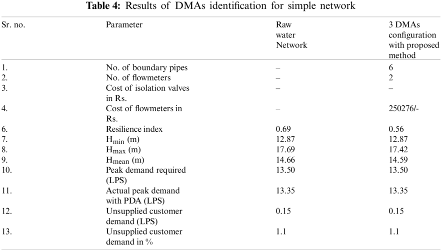
The network in the first example is a small illustrative system for testing and demonstrating the proposed model. The system layout is the same as shown in Fig. 2a. Following the segment identification scheme resulted in three segments as shown in Fig. 2b. After the identification of the segments, it is required to isolate the segments from each other by minimizing their interconnections.
In this case, 6 boundary pipes were identified. The preliminary hydraulic analysis of the network was done to get an idea of the network performance in terms of demand and pressure satisfaction. The minimum pressure requirements for adequate customer satisfaction were fixed to 14 m. The total demand of the network is 13.50 LPS.
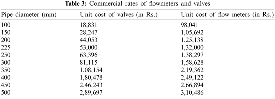
The proposed sectorization method has been applied to the network. The commercial rates of flow meters and isolation valves have been extracted from the schedule of rates published by the state water utility authority (https://www.mjpmaharashtra.gov.in) (see Table 3).
The GA parameters used for the cost optimization problem are as follows: population size = 50; number of generations = 50; crossover and mutation probability = 0.8 and 0.1, respectively; lower and upper bounds of variables = 0 and 1, respectively; penalty multiplier = 7.261 × 10⁶. In this case, a slight violation of nodal head constraints was allowed to explore the solutions near the boundary of feasible and infeasible solutions. Such violations cause slight unsupplied customer demand (allowable up to 1.5% of the total demand) in the network.
The valve closure functionality in EPANET is embedded as a pipe property. In order to simulate the closure of valves, the boundary pipe linked to valves need to be closed. Hence, in this case the valves closure and boundary pipes closure are used interchangeably. The boundaries optimization resulted in a configuration in which four boundary valves could be closed out of 6 potential boundary valves. The total cost of two flow meters required would be Rs. 2,50,276/-.
Once the boundaries are fixed, the next step corresponds to the performance evaluation of the final solution in terms of resilience index and other statistical performance indices. The resilience index of the raw network was 0.69 and for the partitioned network with 4 valves closed, the network resilience dropped to 0.56. When few valves are closed, the water takes longer routes to reach the demand nodes changing the original configuration of the network. This increases the head loss in the network and causes a pressure drop and reduction in total energy in the system.
It is important to explore the changes in statistical performance indicators like mean, maximum, and minimum pressure values in the network. The nodal pressure can be treated as a proxy to leakage reduction. From Table 4, it is clear that the fluctuations in the statistical indices of the network are insignificant due to the small size of the network. The minimum pressure in the raw network was 12.87 m. The maximum pressure before and after partitioning was 17.69 and 17.42 m.
Also, the unsupplied water demand in the network did not fluctuate beyond 1.1% before and after closing the pipes. This was due to the strict penalty function which directed the solution towards the least violation of penalty.
Example 2: Medium size real water network
Ramnagar GSR operational hydraulic zone [34] is located in the western part of Nagpur city, India, comprising of residential, institutional, and commercial customers. The network layout consists of 411 nodes, 435 pipes, 1 reservoir, and 59 valves as shown in Fig. 3. Since the network under consideration is a real-life working network, the authors have not altered any network properties including the positioning of valves. A preliminary hydraulic analysis of the existing water network was performed to get an idea of the pressure and nodal demand satisfaction levels where the minimum pressure required for full demand satisfaction was set to 8.0 m.

Figure 3: Existing water network layout
Preliminary hydraulic analysis of the network showed that the existing network has lower operating pressures for peak hour demand at few demand nodes which results in unsupplied customer demand of 0.3% of the total demand (where total demand = 219.31 liters per second).
Segmentation of the given water network using the proposed methodology resulted in 21 segments as shown in Fig. 4. However, the proposed methodology provides some individual pipes as segments, individual pipes enclosed between two valves as segments, and also considers the source as a segment, which is not in line with the idea of DMAs design. Also, if such segments are considered as DMAs, then it would increase the computational complexity as the preceding pipe supplying water to such segments will have to be considered as a potential boundary pipe during the sectorization phase. It is observed that some segments have very few pipes because of the locations of valves.

Figure 4: 21 segments obtained with segments identification method
Therefore, such segments have been merged into the adjacent segments with engineering judgment to reduce the sample size of potential boundary pipes as shown in Fig. 5. The merging process resulted in 13 segments or zones with 30 potential boundary pipes (valves in this case) whose status’ (open/closed) have been fixed using single-objective GA.

Figure 5: 13 DMAs configuration obtained after merging a few segments
The proposed sectorization method has been implemented for the worst-case scenario, i.e., for peak demand conditions where the total outflow from the reservoir for peak demand hour was 219.31 liters per second (LPS). A minor constraint violation, i.e., unsupplied customer demand of 1% of the total demand was allowed in the design. The GA parameters used for the cost optimization problem are the same as used in the first example.
The segment identification procedure blended with engineering judgment resulted in 13 DMAs and 30 boundary pipes out of which 15 pipes were closed to establish permanent boundaries. The following results are obtained. For the obtained DMA configuration, a total of 15 numbers of flow meters costing Rs. 15,19,792/- would be required. The RI value of the existing water network is found to be low, i.e., 0.37 and it is found to be 0.31 for the partitioned network. The pressure values in the existing water network, i.e., the minimum, mean, and maximum pressure values (in m) are 5.632, 13.128, and 20.16 m respectively while for the proposed configuration, the pressure values dropped to 5.606, 12.78, and 19.787 m, respectively.
The existing water network itself has nodal pressure below 8 m at a few nodal points, resulting in slight unsupplied customer demand. A total of 218.651 LPS demand is being fulfilled as against the requirement of 219.31 LPS with a demand shortfall of 0.659 LPS. However, it is made sure that the unsupplied customer demand should not exceed 1% of the total required demand. This is also reflected even after closing 15 boundary pipes. The total unsupplied customer demand for the proposed network configuration is 0.91 LPS which is slightly high against the existing network (i.e., 0.659 LPS).
Louvain Algorithm Based DMAs Configuration
Example 3
Apart from the proposed methodology, an additional network configuration has also been worked out in which all the existing valves of the network have been removed without disturbing the hydraulic input data.
The algorithm is a heuristic greedy method based on modularity optimization. The fundamental principle of this algorithm is that the edges are strongly connected inside the clusters whereas inter-cluster connections are sparse. It uses the modularity index as an evaluation criteria of network partitioning. The modularity index is mathematically expressed as:
where Aυω = element of the adjacency matrix of the network (Aυω = 1 if vertices υ and ω are connected; otherwise, Aυω = 0);
The advantage of Louvain algorithm over other clustering algorithms is that it allows the users to adjust and obtain the desired clustering configuration with a mere adjustment of resolution parameter. In this work, Gephi software (https://www.gephi.org) is used to get the desired clusters by adjusting resolution parameter. Nodal average pressure between the two connected nodes were assigned as weights to the corresponding links. For more details on multi-resolution modularity, readers can refer to Zhang et al. [9].
In order to arrive at the same number of 13 clusters as obtained in the existing valve infrastructure, the resolution parameter is adjusted as a trial and error approach and 13 clusters are identified. However, the arrangement of clusters and the boundaries are different. The pictorial representation of this configuration is shown in Fig. 6.
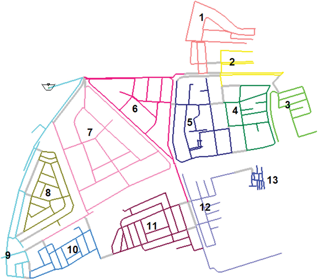
Figure 6: 13 DMAs configuration for Louvain based algorithm
The sectorization or boundaries optimization of this configuration is done using the same procedure (GA) as explained in this paper. This additional work is presented to get an idea of how the network would have behaved when treated as a raw network without any existing valves. The Louvain algorithm-based configuration relatively had a similar number of closed boundary pipes with a drop in resilience index, i.e., 0.28. The total cost of strategy implementation for this configuration was Rs. 23,56,684. It is quite obvious that closed pipes reduce the resilience index of the network as the water has to take a longer route for reaching the desired nodes. The Louvain configuration resulted in a costlier solution in terms of the cost of valves and flow meters, but it should be noted that the additional cost of infrastructure required for installing the devices is not considered. Such additional costs for existing networks will be considerably less and it is a passive advantage of using existing infrastructure for DMAs identification. The better performance of the existing infrastructure-based configuration comes at a cheaper cost and a better resilience index. It can be said that the cost of DMAs design and the network’s hydraulic performance are inversely related.
The results of the proposed method using existing valves and the results of Louvain algorithm based configuration is presented in Table 5.
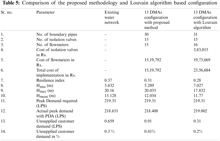
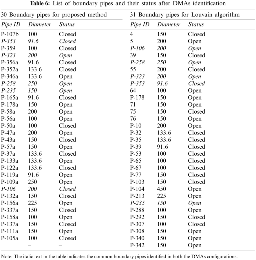
Table 6 enlists the boundary pipes, their diameters, and their corresponding open/closed status for both configurations. Five boundary pipes were common in both the cases, and they are shown in Italics in Table 6. Out of the five common pipes three pipes were open for both the cases. It shows that the pipes are hydraulically important as closing these pipes may drastically affect the network performance. The best part of the existing infrastructure-based method is that a mere closure of selective valves in the water network leads to desired DMAs formation with the least disturbance in existing daily operations of the water network. As against this, the aim of many developed methodologies in the past was to decide DMAs identification for raw water networks without considering the actual valves in the network. The clustering algorithms used features like flow rate, diameter, nodal heads to assign pipe weights.
The proposed methodology has multiple steps and requires some expertise from the user. The algorithm used in segments identification terminates once the valves are identified and starts the search in other directions. The method does not guarantee any kind of hydraulic similarities like demand or pressure similarity among the nodes in identified segments. Also, the algorithm gives a single pipe segment or segments with few pipes depending on the location of the valves as highlighted in Fig. 4.
Usually, it is preferred to have a DMA with some minimum connections or some minimum pipe lengths [4]. Herein, a judgment is made by merging some of the adjacent segments to have a DMA with some minimum connections. Development of heuristic or optimization-based methodology to combine adjacent segments can be explored in the future so that the dependency of human expertise can be reduced for DMAs identification. The optimization of hydraulic properties of the network like pressure and demand similarity along with the number of customer connections per DMA can also be considered.
The use of single-objective GA for minimizing the cost of implementation with PDA converged quickly towards the optimum solution. The penalty function worked effectively to discard infeasible solutions and the optimum value was attained in just 13 generations.
However, the recent research interests in the areas of optimal DMAs design indicate that many aspects should be simultaneously optimized. This gives rise to the need of using many-objective optimization methodologies for the sectorization phase.
This paper presents an advancement in DMAs design methodology which taps the potential of existing valves of the water network. The paper includes (1) mapping the water network into a graph and clusters identified using the proposed segmentation procedure blended with engineering judgment; (2) Determining the boundary pipes that can be closed to establish permanent boundaries; and (3) Performance evaluation of the partitioned network.
The methodology is implemented on a real water network and results show that the proposed method can reasonably form DMAs without adversely affecting the hydraulic capacity of the water network. It is opined that there is a huge potential for new methodologies to be devised for DMAs identification as discussed in the previous section. Regarding the use of optimization tools, it is important to consider several factors at a time while fixing the boundary status, which needs robust optimization techniques.
This method could be beneficial for water utilities having budget constraints but are willing to improve the operational efficiency of the existing water network. Finally, it is worth noting that with the proposed technique, fair results of DMAs identification can only be achieved by carefully applying the method with sound engineering judgment.
Availability of Data and Material: The data presented in this study are available on request from the corresponding author.
Code Availability: The source codes used in this work are available on request from the corresponding author.
Funding Statement: The authors received no specific funding for this work.
Conflicts of Interest: The authors declare that they have no conflicts of interest to report regarding the present study.
1. Bhagat, S. K., Welde, T. W., Tesfaye, O., Tung, T. M., Al-Ansari, N. et al. (2019). Evaluating physical and fiscal water leakage in water distribution system. Water, 11(10), 2091. DOI 10.3390/w11102091. [Google Scholar] [CrossRef]
2. Gupta, A., Bokde, N., Kulat, K., Yaseen, Z. M. (2020). Nodal matrix analysis for optimal pressure-reducing valve localization in a water distribution system. Energies, 13(8), 1878. DOI 10.3390/en13081878. [Google Scholar] [CrossRef]
3. Laucelli, D., Simone, A., Berardi, L., Giustolisi, O. (2017). Optimal design of district metering areas for the reduction of leakages. Journal of Water Resources Planning and Management, 143(3), 04017017. DOI 10.1061/(ASCE)WR.1943-5452.0000768. [Google Scholar] [CrossRef]
4. Morrison, J., Tooms, S., Rogers, D. (2007). District metered areas: Guidance notes. Technical Report 1. Water Loss Task Force, International Water Association (IWALondon, UK. [Google Scholar]
5. Ferrari, G., Savic, D., Becciu, G. (2014). Graph-theoretic approach and sound engineering principles for design of district metered areas. Journal of Water Resources Planning and Management, 140(12), 04014036. DOI 10.1061/(ASCE)WR.1943-5452.0000424. [Google Scholar] [CrossRef]
6. Perelman, L., Allen, M., Preis, A., Iqbal, M., Whittle, A. (2015). Flexible reconfiguration of existing urban infrastructure systems. Environmental Science and Technology, 49(22), 13378–13384. DOI 10.1021/acs.est.5b03331. [Google Scholar] [CrossRef]
7. Ciaponi, C., Murari, E., Todeschini, S. (2016). Modularity based procedure for partitioning water distribution systems into independent districts. Water Resources Management, 30(6), 2021–2036. DOI 10.1007/s11269-016-1266-1. [Google Scholar] [CrossRef]
8. Zhang, K., Yan, H., Zeng, H., Xin, K., Tao, T. (2018). A practical multi-objective optimization sectorization method for water distribution network. Science of the Total Environment, 656, 1401–1412. DOI 10.1016/j.scitotenv.2018.11.273. [Google Scholar] [CrossRef]
9. Zhang, Q., Wu, Y., Zhao, M. Q. J., Huang, Y., Zhao, H. (2017). Automatic partitioning of water distribution networks using multiscale community detection and multi objective optimization. Journal of Water Resources Planning and Management, 143(9), 04017057. DOI 10.1061/(ASCE)WR.1943-5452.0000819. [Google Scholar] [CrossRef]
10. Vasilic, Z., Stanic, M. K., Prodanovic, D., Babic, B. (2020). Uniformity and heuristics-based DeNSE method for sectorization of water distribution networks. Journal of Water Resources Planning and Management, 146(3), 04019079. DOI 10.1061/(ASCE)WR.1943-5452.0001163. [Google Scholar] [CrossRef]
11. Wright, R., Stoinav, I., Parpas, P., Henderson, K., King, J. (2014). Adaptive water distribution networks with dynamically reconfigurable topology. Journal of Hydroinformatics, 16(6), 1280–1301. DOI 10.2166/hydro.2014.086. [Google Scholar] [CrossRef]
12. Alvisi, S., Franchini, M. (2013). Heuristic procedure for the automatic creation of district metered areas in water distribution systems. Urban Water Journal, 11(2), 137–159. DOI 10.1080/1573062X.2013.768681. [Google Scholar] [CrossRef]
13. di Nardo, A., di Natale, M., Santonastaso, G. F., Tzatchkov, V. G., Alcocer-Yamanaka, V. H. (2014). Water network sectorization based on graph theory and energy performance indices. Journal of Water Resources Planning and Management, 140(5), 620–629. DOI 10.1061/(ASCE)WR.1943-5452.0000364. [Google Scholar] [CrossRef]
14. Bui, K., Marlim, M. S., Kang, D. (2021). Optimal design of district metered areas in a water distribution network using coupled self-organizing map and community structure algorithm. Water, 13(6), 836. DOI 10.3390/w13060836. [Google Scholar] [CrossRef]
15. Diao, K., Zhou, Y., Rauch, W. (2013). Automated creation of district metered area boundaries in water distribution systems. Journal of Water Resources Planning and Management, 139(2), 184–190. DOI 10.1061/(ASCE)WR.1943-5452.0000247. [Google Scholar] [CrossRef]
16. Yao, H., Zhang, T., Shao, Y., Tingchao, Y., Lima Neto, I. E. (2020). Improved modularity based approach for partition of water distribution networks. Urban Water Journal, 18(2), 69–78. DOI 10.1080/1573062X.2020.1857801. [Google Scholar] [CrossRef]
17. Zeidan, M., Li, P., Ostfeld, A. (2021). DMA segmentation and multiobjective optimization for trade off water age, excess pressure, and pump operational cost in water distribution systems. Journal of Water Resources Planning and Management, 147(4), 04021006. DOI 10.1061/(ASCE)WR.1943-5452.0001344. [Google Scholar] [CrossRef]
18. Scarpa, F., Lobba, A., Becciu, G. (2016). Elementary DMA design of looped water distribution networks with multiple sources. Journal of Water Resources Planning and Management, 142(6), 04016011. DOI 10.1061/(ASCE)WR.1943-5452.0000639. [Google Scholar] [CrossRef]
19. Giustolisi, O., Ridolfi, L. (2014). A new modularity-based approach to segmentation of water distribution networks. Journal of Hydraulic Engineering, 140(10), 04014049. DOI 10.1061/(ASCE)HY.1943-7900.0000916. [Google Scholar] [CrossRef]
20. Bui, K., Marlim, M. S., Kang, D. (2020). Water network partitioning into district metered areas: A state-of-the-art review. Water, 12(4), 1002. DOI 10.3390/w12041002. [Google Scholar] [CrossRef]
21. Gomes, R., Marques, A., Sousa, J. (2012). Decision support system to divide a large network into suitable district metered areas. Water Science and Technology, 65(9), 1667–1675. DOI 10.2166/wst.2012.061. [Google Scholar] [CrossRef]
22. Di Nardo, A., Di Natale, M., Giudicianni, C., Santonastaso, G. F., Tzatchkov, V. et al. (2017). Economic and energy criteria for district meter areas design of water distribution networks. Water, 9(7), 463. DOI 10.3390/w9070463. [Google Scholar] [CrossRef]
23. Campbell, E., Izquierdo, J., Montalvo, I., Ilaya-Azya, A., Perez-Garci, R. et al. (2016). A flexible methodology to sectorize water supply networks based on social network theory concepts and multi-objective optimization. Journal of Hydroinformatics, 18(1), 62–76. DOI 10.2166/hydro.2015.146. [Google Scholar] [CrossRef]
24. Pesantez, J., Berglund, E., Mahinthakumar, G. (2019). Multiphase procedure to design district metered areas for water distribution networks. Journal of Water Resources Planning and Management, 145(8), 04019031. DOI 10.1061/(ASCE)WR.1943-5452.0001095. [Google Scholar] [CrossRef]
25. Zevnik, J., Fijavz, M. K., Kozelj, D. (2019). Generalized normalized cut and spanning trees for water distribution network partitioning. Journal of Water Resources Planning and Management, 145(10), 04019041. DOI 10.1061/(ASCE)WR.1943-5452.0001100. [Google Scholar] [CrossRef]
26. Hajebi, S., Roshani, E., Cardazo, N., Barrett, S., Clarke, A. et al. (2015). Water distribution network sectorisation using graph theory and many-objective optimisation. Journal of Hydroinformatics, 18(1), 77–94. DOI 10.2166/hydro.2015.144. [Google Scholar] [CrossRef]
27. Liu, J., Lansey, K. (2020). Multiphase DMA design methodology based on graph theory and many-objective optimization. Journal of Water Resources Planning and Management, 146(8), 04020068. DOI 10.1061/(ASCE)WR.1943-5452.0001267. [Google Scholar] [CrossRef]
28. Gajghate, P. W., Mirajkar, A., Shaikh, U., Bokde, N. D., Yaseen, Z. M. (2021). Optimization of layout and pipe sizes for irrigation pipe distribution network using Steiner point concept. Mathematical Problems in Engineering, 2021(9), 1–12. DOI 10.1155/2021/6657459. [Google Scholar] [CrossRef]
29. Liu, J., Han, R. (2018). Spectral clustering and multicriteria decision for design of district metered areas. Journal of Water Resources Planning and Management, 144(5), 04018013. DOI 10.1061/(ASCE)WR.1943-5452.0000916. [Google Scholar] [CrossRef]
30. Brentan, B., Carpitella, S., Izquierdo, J., Luvizotto, E., Meirelles, G. (2021). District metered area design through multicriteria and multiobjective optimization. In: Mathematical methods in the applied sciences. John Wiley and Sons, UK. DOI 10.1002/mma.7090. [Google Scholar] [CrossRef]
31. di Nardo, A., di Natale, M. (2010). A heuristic design support methodology based on graph theory for district metering of water supply networks. Engineering Optimization, 43(2), 193–211. DOI 10.1080/03052151003789858. [Google Scholar] [CrossRef]
32. di Nardo, A., di Natale, M., Santonastaso, G. F., Tzatchkov, V. G., Alcocer-Yamanaka, V. H. (2015). Performance indices for water network partitioning and sectorization. Water Science & Technology: Water Supply, 15(3), 499–509. DOI 10.2166/ws.2014.132. [Google Scholar] [CrossRef]
33. Santonastaso, G. F., di Nardo, A., Creaco, E. (2019). Dual topology for partitioning of water distribution networks considering actual valve locations. Urban Water Journal, 16(7), 469–479. DOI 10.1080/1573062X.2019.1669201. [Google Scholar] [CrossRef]
34. Jadhao, R., Gupta, R. (2018). Calibration of water distribution network of the Ramnagar zone in Nagpur City using online pressure and flow data. Applied Water Science, 8(1), 1–10. DOI 10.1007/s13201-018-0672-3. [Google Scholar] [CrossRef]
35. Kaldenbach, J., Ormsbee, L. (2012). Automated segmentation analysis of water distribution systems. World Environment and Water Resources Congress, pp. 629–634. Albuquerque, New Mexico, USA. [Google Scholar]
36. Gupta, R., Baby, A., Arya, P. V., Ormsbee, L. (2014). Segment-based reliability/supply short fall analysis of water distribution networks. Procedia Engineering, 89, 1168–1175. DOI 10.1016/j.proeng.2014.11.244. [Google Scholar] [CrossRef]
37. Pohl, I. (1970). Heuristic search viewed as path finding in a graph. Artificial Intelligence, 1(3), 193–204. DOI 10.1016/0004-3702(70)90007-X. [Google Scholar] [CrossRef]
38. Sharafati, A., Tafarojnoruz, A., Motta, D., Yaseen, Z. M. (2020). Application of nature-inspired optimization algorithm to ANFIS model to predict wave-induced score depth around pipelines. Journal of Hydroinformatics, 22(6), 1425–1451. DOI 10.2166/hydro.2020.184. [Google Scholar] [CrossRef]
39. Kadu, M. S., Gupta, R., Bhave, P. R. (2008). Optimal design of water networks using a modified genetic algorithm with reduction in search space. Journal of Water Resources Planning and Management, 134(2), 147–160. DOI 10.1061/(ASCE)0733-9496(2008)134:2(147). [Google Scholar] [CrossRef]
40. Sayyed, M. A. H., Gupta, R., Taniamboh, T. (2015). Noniterative application of EPANET for pressure dependent modelling of water distribution systems. Water Resources Management, 29(9), 3227–3242. DOI 10.1007/s11269-015-0992-0. [Google Scholar] [CrossRef]
41. Gupta, R. (2015). History of pressure-dependent analysis of water distribution networks and its applications. World Environmental and Water Resources Congress, Austin, TX. [Google Scholar]
42. Wagner, J. M., Shamir, U., Marks, D. H. (1988). Water distribution reliability: Simulation method. Journal of Water Resources Planning and Management, 114(3), 276–294. DOI 10.1061/(ASCE)0733-9496(1988)114:3(276). [Google Scholar] [CrossRef]
43. Sayyed, M. A. H., Gupta, R., Taniamboh, T. (2019). Combined flow and pressure deficit-based penalty in GA for optimal design of water distribution network. Journal of Hydraulic Engineering, 1–11. DOI 10.1080/09715010.2019.1604180. [Google Scholar] [CrossRef]
44. Todini, E. (2000). Looped water distribution networks design using a resilience index based heuristic approach. Urban Water Journal, 2(2), 115–122. DOI 10.1016/S1462-0758(00)00049-2. [Google Scholar] [CrossRef]
 | This work is licensed under a Creative Commons Attribution 4.0 International License, which permits unrestricted use, distribution, and reproduction in any medium, provided the original work is properly cited. |