| Computer Modeling in Engineering & Sciences |
DOI: 10.32604/cmes.2022.019435
ARTICLE
Deep-Learning-Based Production Decline Curve Analysis in the Gas Reservoir through Sequence Learning Models
1State Key Laboratory of Shale Oil and Gas Enrichment Mechanisms and Effective Development, Beijing, 100083, China
2Sinopec Petroleum Exploration and Production Research Institute, Beijing, 100083, China
3Department of Oil-Gas Field Development Engineering, College of Petroleum Engineering, China University of Petroleum, Beijing, 102249, China
*Corresponding Author: Liang Xue. Email: xueliang@cup.edu.cn
Received: 24 September 2021; Accepted: 24 November 2021
Abstract: Production performance prediction of tight gas reservoirs is crucial to the estimation of ultimate recovery, which has an important impact on gas field development planning and economic evaluation. Owing to the model's simplicity, the decline curve analysis method has been widely used to predict production performance. The advancement of deep-learning methods provides an intelligent way of analyzing production performance in tight gas reservoirs. In this paper, a sequence learning method to improve the accuracy and efficiency of tight gas production forecasting is proposed. The sequence learning methods used in production performance analysis herein include the recurrent neural network (RNN), long short-term memory (LSTM) neural network, and gated recurrent unit (GRU) neural network, and their performance in the tight gas reservoir production prediction is investigated and compared. To further improve the performance of the sequence learning method, the hyper-parameters in the sequence learning methods are optimized through a particle swarm optimization algorithm, which can greatly simplify the optimization process of the neural network model in an automated manner. Results show that the optimized GRU and RNN models have more compact neural network structures than the LSTM model and that the GRU is more efficiently trained. The predictive performance of LSTM and GRU is similar, and both are better than the RNN and the decline curve analysis model and thus can be used to predict tight gas production.
Keywords: Tight gas; production forecasting; deep learning; sequence learning models
With the increasing demand for natural gas resources to empower economic development, tight gas reservoirs have become an important source of energy and have been discovered in major basins to produce oil and gas worldwide. The tight gas reservoir falls into the category of unconventional natural gas resources due to its low-permeability and low-porosity characterization [1,2], as well as the special pore structure associated with it [2]. The productivity of tight gas reservoirs is too low to be developed in a profitable manner and requires the use of a hydraulic fractured horizontal well to increase production [3–5]. To reasonably set up a tight-gas-reservoir development plan, one of the most challenging tasks is to accurately predict the future gas production behavior in such a reservoir, which can help the decision-maker to obtain the information on estimated ultimate recoveries (EURs), determine the abandoned time of the production well, and evaluate the economic benefits of the well.
To forecast tight gas production, reservoir simulation models have been developed over the past decades [6–8]. However, the flow behavior in a tight gas reservoir is complex. It has been found that such a reservoir has a threshold pressure gradient [9,10]; the permeability in a tight gas reservoir may change with pressure and exhibits a stress-sensitive effect during the production process [11,12]; the proppant embedment issues in the hydraulic fractures of a tight reservoir may affect the gas production [13]; the temperature and pressure may affect the imbibition recovery for tight or shale gas reservoir [14]; the tight gas production may be seriously reduced by water blockage [15–17]; the dispersed distribution of kerogen within matrices may affect the production evaluation [18]; sulfur precipitation and reservoir pressure-sensitive effects may affect the permeability, porosity and formation pressure [19]; the micro-scale flow mechanism, such as Knudsen diffusion, slippage effect, and adsorption, can be difficult to describe quantitatively [20,21]. All these complexities associated with tight gas reservoirs make it difficult to build an accurate mathematical model to predict gas flow in tight gas reservoirs. Decline curve analysis is an effective and widely used method to forecast reservoir production behavior because of the simplicity of the mathematical form. For a conventional reservoir, the Arps model has been successfully used to conduct well production forecasting for decades [22]. For an ‘unconventional’ reservoir, several new models have been proposed to improve prediction accuracy. The traditional hyperbolic decline model has been improved as the modified hyperbolic decline model [23]. The power-law exponential model has been proposed to estimate the gas reserve in low-permeability reservoirs [24]. The stretched exponential decline model was established to analyze Barnet shale gas production [25], and its performance has been validated [26]. The Duong model was built to estimate the EUR for unconventional reservoirs when the fracture flow is the most significant flow regime, such as in tight and shale gas wells [27].
With an increasing number of tight gas production wells, a data-driven production forecasting model can be built using machine-or deep-learning methods. Wang et al. [28] developed a comprehensive data-mining process and found that random forest approach outperforms adaptive boosting (AdaBoost), support vector machine (SVM), and artificial neural network (ANN) approaches in evaluating the well production in Montney Formations. Luo et al. [29] built a neural network model consisting of four hidden layers with 100 neurons in each layer to identify the relationship between oil production and the important features of datasets from 2,000 horizontal wells targeting the Mid-Bakken Formation. Noshi et al. [30] applied gradient boosted trees, Adaboost, and SVM to structure and train different regression algorithms to predict cumulative production within the first 12 producing months. Li et al. [31] compared accumulated production predictions among C4.5 and ANN models in which the three numeric variables, namely, permeability, porosity, and first-shut-in-pressure, were identified as inputs. The results showed that the normal distribution transformation (NDT) model can significantly improve the classification accuracy of the C4.5 algorithm. When compared to the ANN approach, the NDT model has a lower classification rate in general but is better able to describe classes with a low number of instances. Data on a total of 2,919 wells in the Bakken Formation were collected and analyzed to develop a reliable deep neural network model to estimate cumulative oil production [32]. The one-hot encoding method, Xavier initialization, dropout technique, batch normalization, and K-fold cross-validation were all used to improve the model's performance.
Tight gas production data are essentially a type of sequence data, and an algorithm initially developed for natural language processing can be used to analyze this data type. The standard recurrent neural network (RNN) is used to analyze the flow rate and pressure data collected from permanent downhole gauges [33]. Sun et al. [34] predicted the production of a single shale gas well and the cumulative production of multiple wells based on the variant long-and short-term memory (LSTM) neural network of an RNN, which shows a better production trend and smaller production error compared with the decline curve method. LSTM is used as a machine-learning method without resorting to a physical model to supplement missing well logging information [35]. A particle-swarm-optimized LSTM method was proposed to analyze the oil production in a volcanic reservoir that incorporated the well control constraint into the model [36]. The gated recurrent unit (GRU) neural network was proposed to forecast batch production in a conglomerate reservoir [37].
The purpose of the present research is to investigate the performance of tight gas reservoir production forecasting by using deep-learning-based sequence learning models since there is still no consensus on which model is best suited for tight gas production forecasting. The novelty of this work is that it provides a comprehensive evaluation of the forecasting performance of different sequence learning models.
The rest of this paper is organized as follows. First, the theoretical bases of the sequence models are introduced. Second, the tight gas production data processing procedures are explained. Third, the forecasting performance is compared after the hyper-parameters are optimized through a particle-swarm-optimization method. Finally, conclusions are drawn based on the analysis results.
An RNN is a type of neural network with an iterative loop structure. The traditional neural network can only build a direct mapping relationship between input and output. The loop design of an RNN, however, can make it more suitable to deal with sequence data and allow it to obtain more and more persistent information from the past sequence. The RNN was proposed by Hopfield in 1982 to implement pattern recognition and recover a stored pattern from a corrupted one [38]. A basic RNN unit cell in a hidden layer is shown in Fig. 1.
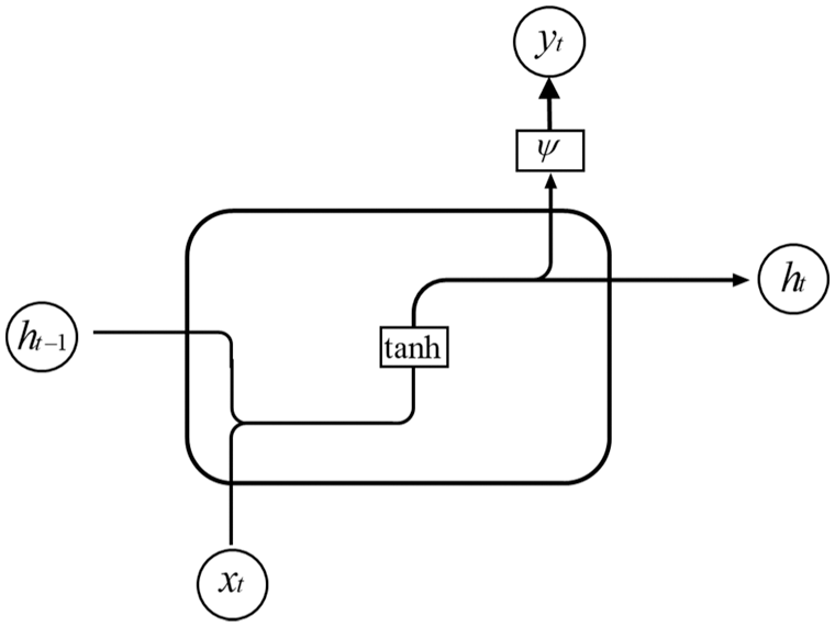
Figure 1: Recurrent neural network unit cell in a hidden layer
In Fig. 1, xt represents the input information at time t, ht the state information of the hidden layer at time t, and yt the output information at time t. Compared with the traditional ANN, an RNN shares the same weight in the calculation process at all time steps, which greatly reduces the network parameters to be learned.
In the forward-propagation process, the state of the hidden layer at time t is
where
The information of the output layer is expressed as
where
The weight update of the RNN adopts the back-propagation through time method and the gradient-descent method to continuously optimize the weights along the negative gradient direction of the weight until convergence. In the RNN, in the process of error back-propagation calculation, the issue of gradient vanishing or gradient explosion will arise, that is, the RNN cannot learn from the data with long-term correlations, resulting in the increase of prediction error [39–41]. When establishing the production prediction model of a tight gas reservoir, the input data are often the daily production data for several years or even decades. The input of a large number of data points in the RNN may have unfavorable effects on the prediction of tight-gas-reservoir production.
2.2 Long Short-Term Memory Neural Network
To solve the gradient-vanishing or-explosion problem of the RNN, Hochreiter et al. [42] proposed an improved RNN structure called the LSTM neural network, which is a variant of the RNN that can solve the gradient problem of the RNN. Compared with the RNN, LSTM introduces a memory unit and a control gate into the neural network structure that can control the information transmission between the hidden layers of the neural network. The network structure is shown in Fig. 2.
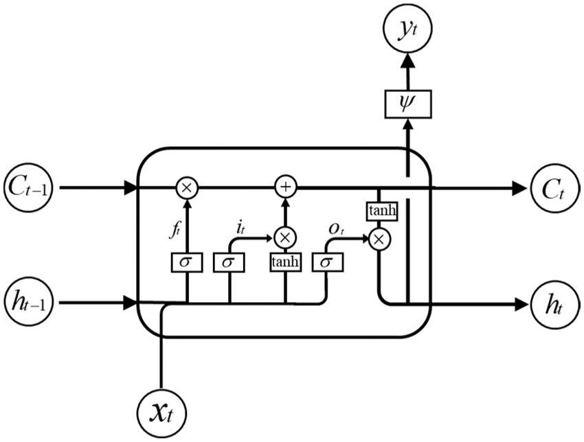
Figure 2: Structure of unit cell in the long short-term memory neural network
In the neural network hidden layer of LSTM, an input gate, an output gate, and a forget gate are added to control the memory unit. At time t, the value of the forget gate in the memory unit is calculated through the input information
The value of the forget gate can be computed by
where
The value of the input gate can be computed as
where
The candidate cell state
At this time, the updated candidate cell state, and the cell state
The value of the output gate is
where
The value of the hidden state is
The value of the output information is
where
According to its operational structure, the LSTM neural network can be used to learn, capture, and extract data features from the time-series data, and a more accurate prediction model can be obtained.
2.3 Gated Recurrent Unit Neural Network
The GRU is a variant of the LSTM, proposed by Cho et al. [43] and Chung et al. [44] in 2014. Compared with the LSTM model, the GRU integrates forget and input gates into a single update gate. Moreover, it also integrates the cell state and makes some other improvements. In the GRU model, there are only two gates, i.e., the update and reset gates, which are simpler than those in the standard LSTM model. The specific structure is shown in Fig. 3.
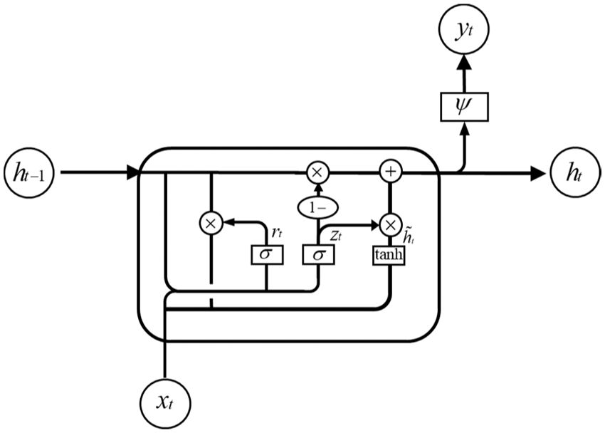
Figure 3: Structure of unit cell in the gated recurrent unit neural network
If
where
The network calculation process of the GRU model is simpler than that of the LSTM model; so, the GRU model is easier to train than the LSTM model; in addition, the convergence time of the model is shorter.
There are reservoir scale and single-well scale analysis on the production prediction in gas reservoir development. The reservoir-scale gas reservoir production is influenced by many factors, such as drilling a new infill well and changing the production schedule. All these factors may make the system too complex to be analyzed accurately. Therefore, in this work, the production curve analysis for the single-well case in the tight gas reservoir is discussed although the methods investigated here are not limited by this case. The deep learning model is built for each production well in the tight gas reservoir. The aim of this research is to predict how the production declines when the historical production data have been recorded and the production schedule remains relatively stable.
In the production process of tight gas wells, the values of dynamic variables, such as production rate and pressure of gas wells, often fluctuate due to various factors. Therefore, it is necessary to process the original data to remove the noise influence of the data. A Savitzky-Golay filter is used to process the production rate data collected from the wellhead in a tight gas reservoir; this type of filter (usually referred to as an SG filter) was first proposed by Savitzky et al. in 1964 [45] and has been widely used since in data smoothing and de-noising. It uses a filtering method based on local polynomial least-squares multiplication fitting in the time domain. The most significant feature of this filter is that it can filter noise and ensure that the shape and width of the signal remain unchanged [46].
The SG filter can be expressed as
where
Since the production data of different wells have different value ranges, it is necessary to normalize the data, such as the production history data containing the target parameters to be predicted and other relevant parameters. Normalization is a dimensionless processing method that makes the absolute value of the physical system a relative value relationship. Normalization is an effective way of simplifying the calculation and reducing the value. Normalization is essentially a linear transformation, which has many good properties. These properties indicate that the change of data can improve the data performance. The functions of normalization are the following. First, it can map the data to the range 0–1 and provide a more convenient and fast data processing. Second, the dimensional expression is changed into a dimensionless expression, which is convenient for the comparison and weighted calculation of indicators of different units or orders of magnitude. Third, it can avoid numerical problems caused by extremely large numbers in the calculation.
The equation to perform the normalization is
where
3.2 Training of Sequence Learning Models
The pre-processed data in the collected tight gas production dataset is divided into two parts. The first 70% of the data are used as the training set to train the model, 15% of the data are used as the test set to predict and verify the effect of the model on the test set, and the optimization algorithm is used to update the model parameters according to the test-set error. The last 15% of the data are used as the prediction set of the model and to evaluate the prediction performance of the sequence learning models. After using the training set to train the model, according to the fitting effect on the model training set and the prediction error of the model on the test set, the particle swarm optimization (PSO) algorithm is used to optimize the hyper-parameters of the sequence learning models, such as the length of the time window and the number of neurons in the sequence learning network layer. Finally, the trained and optimized model is applied to the prediction set to predict the future production dynamics.
The objective of the production performance analysis model is to use the historical production data to predict the tight gas production trend in a certain period in the future. Production control parameters (production time, tubing pressure and production rate at the previous time step) are used as feature data in this paper. The production rate in this paper is referred to gas production rate recorded at the wellhead under downhole pressure control during the production process. Several time steps are taken as a time window, and the production rate at the final time step in the current time window is taken as label data. A time window corresponds to a sample dataset, and different samples are constructed by moving the time window. Then the data were converted into a 3-dimentional matrix of input features (sample number × time step × feature number) and a corresponding label vector of current production rate with the size (sample number × 1), which were used as the training data of neural network model. The data processing and model construction are demonstrated in Fig. 4, and the LSTM is used to calculate the production dynamic data to be predicted and the corresponding error. Finally, the output prediction model is obtained through error back-propagation and continuous iterative training.
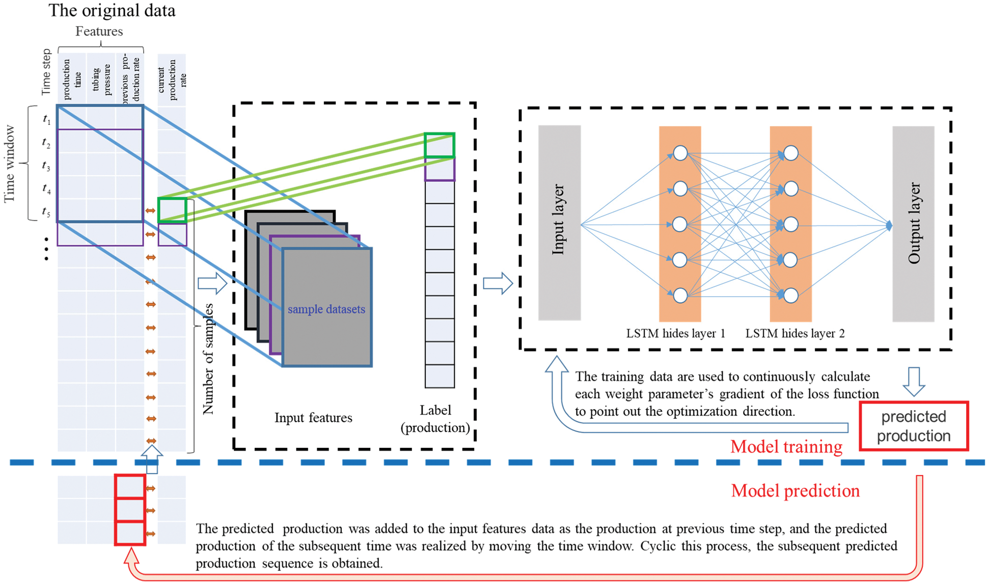
Figure 4: Schematic diagram of original data processing and model construction
It is found that in most studies, when the prediction of output on the prediction set is performed, the actual input data are used directly to predict one or several time steps in the future. This prediction method is equivalent to a short-term prediction in the future, which cannot reflect the long-term decreasing trend of tight gas production in the process of prediction. When forecasting the production on the test and prediction sets, because the gas production data at each step are unknown, the input data of the prediction set cannot be directly constructed. Therefore, it is necessary to use the prediction model to build the input data of the current time step based on the predicted value of the previous time step, that is, the predicted values of the previous time step are added to the time-series data of the output, and the iterative prediction of subsequent production is realized by moving the time window.
3.3 Hyper-Parameter Optimization
The hyper-parameters of the sequence learning model have a great impact on the accuracy of the production prediction model. Whether the hyper-parameters are set properly or not can affect the accuracy of the production prediction model and the convergence speed during model training. When optimizing the hyper-parameters, they must not be allowed to fall into a local optimal solution during model training. A PSO algorithm has good self-learning ability and strong global search ability for the optimal parameters. Therefore, when establishing the prediction model, a PSO algorithm is used to optimize the hyper-parameters of the sequence learning algorithm. The hyper-parameters are updated through continuous iteration until the minimum error standard or the maximum number of iterations of particle update is reached.
The hyper-parameters of the sequence learning model mainly depend on empirical selection, and the hyper-parameters selected by experience are difficult to directly apply to the model, which often requires a cumbersome parameter-tuning process. In this paper, a PSO algorithm is used to automatically optimize the sequence learning model, which saves a significant amount of labor and time cost. Through the prediction performance of the model on the training and test sets, the root-mean-square errors (RMSEs) of the two parts are calculated separately, and then, the objective function f is obtained by a weighted calculation:
Taking the objective function f as the optimization objective of the PSO algorithm, the search dimension is set to 4. The four dimensions represent the length of the time window, the number of neurons in the first layer of the sequence learning neural network layer, the number of neurons in the second layer, and the number of iterations. The hyper-parameters are constantly iterated to optimize the objective function according to the PSO algorithm. The optimization objective function corresponding to this point can be continuously reduced, and the optimization objective function can reach the minimum value in the PSO search space. In this way, the optimal hyper-parameters of the sequence learning model are obtained at the same time, and the corresponding neural network model is the optimal tight gas production forecasting model.
Fig. 5 shows how the objective function value calculated by Eq. (17) changes with the iteration steps during the PSO process for the analysis of production data collected from well X835 in the study area. The figure shows that the objective functions of all the sequence learning models can be reduced after PSO. The optimal hyper-parameters are selected when the objective function cannot be further significantly reduced. At the end of the optimization process, it can be seen that the values of the objective function for the GRU and LSTM models are lower than those for the RNN model, which may be due to the fact that gates are introduced into the GRU and LSTM models. More parameters are required to support the control of the gates and to make the model more flexible for optimization.
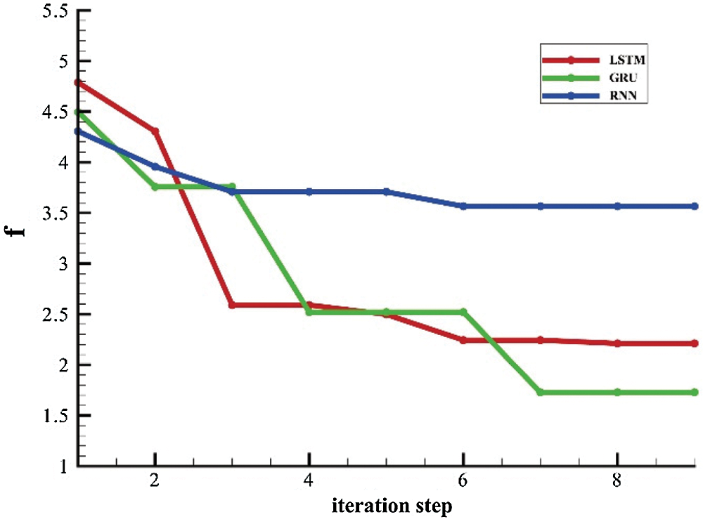
Figure 5: Change of objective-function value during the particle swarm optimization process
For purposes of comparison, the Duong model [27], as a commonly used decline curve analysis model for tight or shale gas reservoirs [47,48], is considered here. The mathematical form of the Duong model can be written as
where q is the production rate,
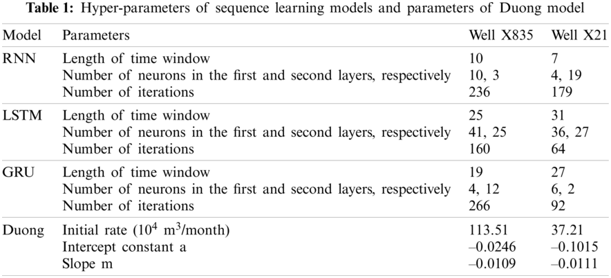
It can be found from Table 1 that in the optimal states of the three sequence learning models, the LSTM model tends to have a more complex unit-cell structure since it requires more neural nodes in the first and second layers than the GRU and RNN models. The LSTM model can process the tight gas production sequence data with a relatively longer time window with less iterative steps. The GRU model has a relatively simple unit cell structure, but it can process the tight gas production sequence data with a much longer time window. From the perspective of network structure complexity, it seems that the GRU model can achieve a balance between efficiency and performance.
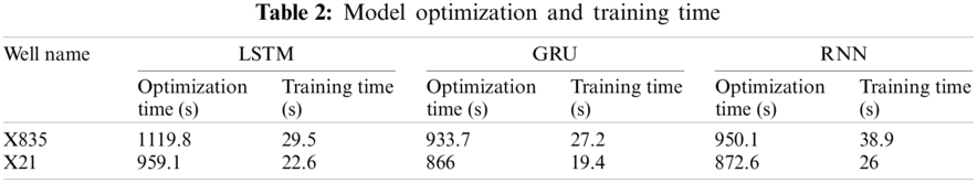
To further investigate the efficiency of the three sequence learning models studied in dealing with tight gas production data, their training and optimization times are compared and are listed in Table 2. Training time here refers to the time required to train the model once to obtain its model parameters, such as the weights and biases. Optimization time refers to the time required by the PSO method to run the model several times to obtain the optimal hyper-parameters. The table further shows that the GRU model has the lowest training time and optimization time overall. If one just examines the training time, it can be seen that the LSTM and GRU models are similar and are both much more efficient to train than the RNN model. However, if we examine the optimization time, it can be seen that the optimization time of the GRU model and that of the RNN model are similar, but the LSTM model takes longer to optimize.
Figs. 6 and 7 depict the production forecasting performances for all the four models by using the data collected from two tight gas production wells, X835 and X21. Among the four models, the Duong model is selected as the representative decline curve analysis model. The RNN, LSTM, and GRU models are deep-learning-based sequence data analysis models. The entire dataset is divided into three parts by vertical dotted lines from left to right in the figures, denoting the training, test, and prediction sets, respectively. The training dataset is used to train the sequence learning model and obtain the neural network model parameters. The test set is used to determine the hyper-parameters in combination with the PSO method. The prediction set is used to evaluate the prediction ability of each model. According to the production prediction results, on the training set, because the data are smoothed and de-noised when training the three sequence learning models and the regular term is used to control the model, the fitting ability to the extreme points of the production curve is limited. However, after ignoring the irregular fluctuation of the production curve, the overall fitting ability of the production curve is obviously improved and exhibits stronger model generalization ability. Regarding the prediction set of three wells, according to the prediction results of the model, it can be seen that the LSTM and GRU models provide prediction results that are close to the actual production data in the two tight gas wells. The GRU and LSTM models show similar prediction performance, despite their optimized network structures being very different from each other. The RNN and Duong models provide prediction results that are far from the actual production curve, which indicates that these two models have relatively poor performances when predicting tight gas production data.
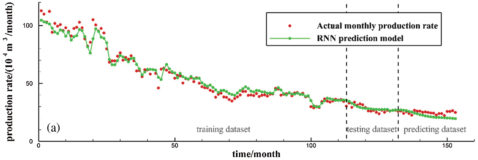
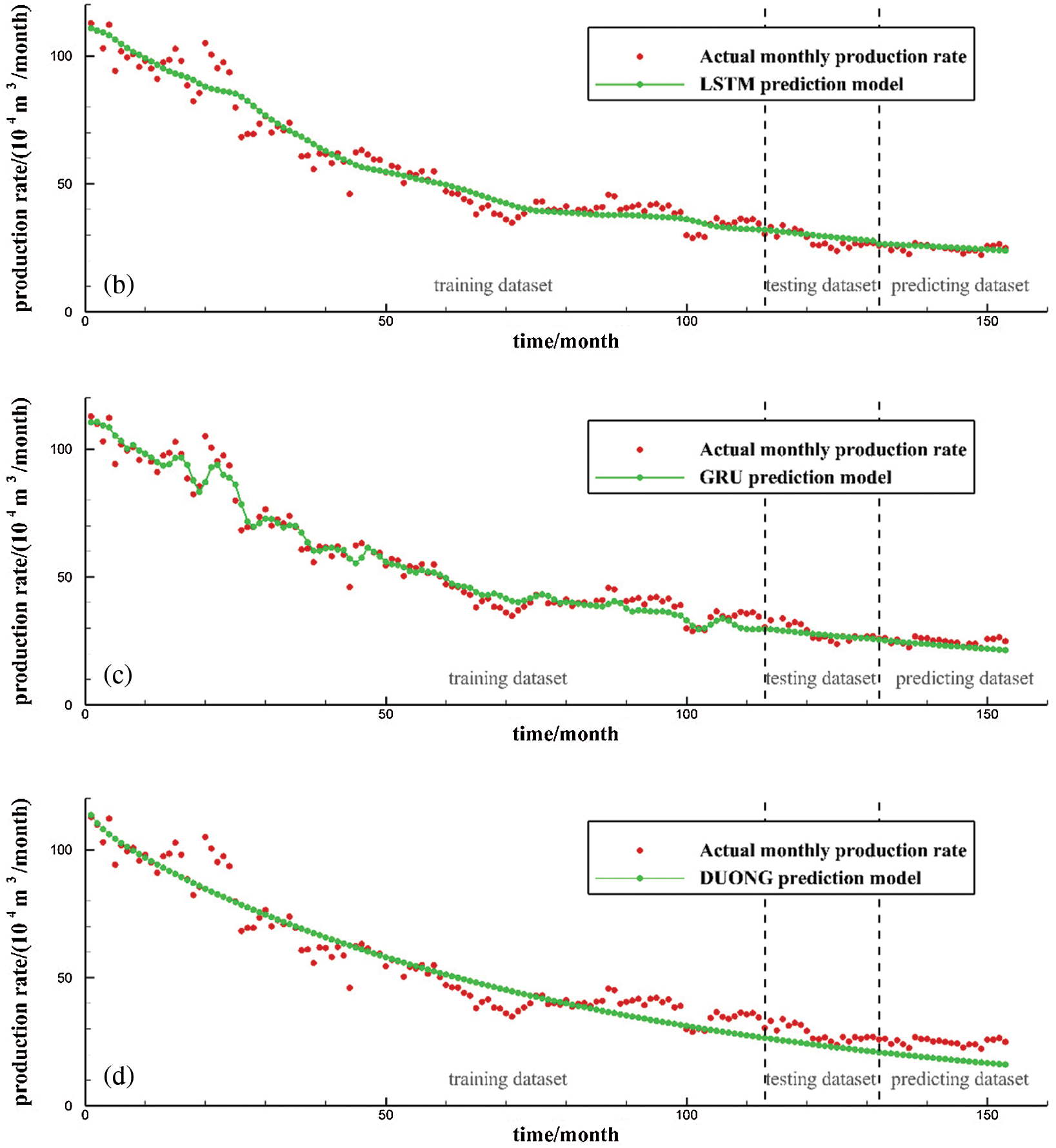
Figure 6: Production prediction performance for Well X835: (a) RNN model; (b) LSTM model; (c) GRU model; (d) Duong model
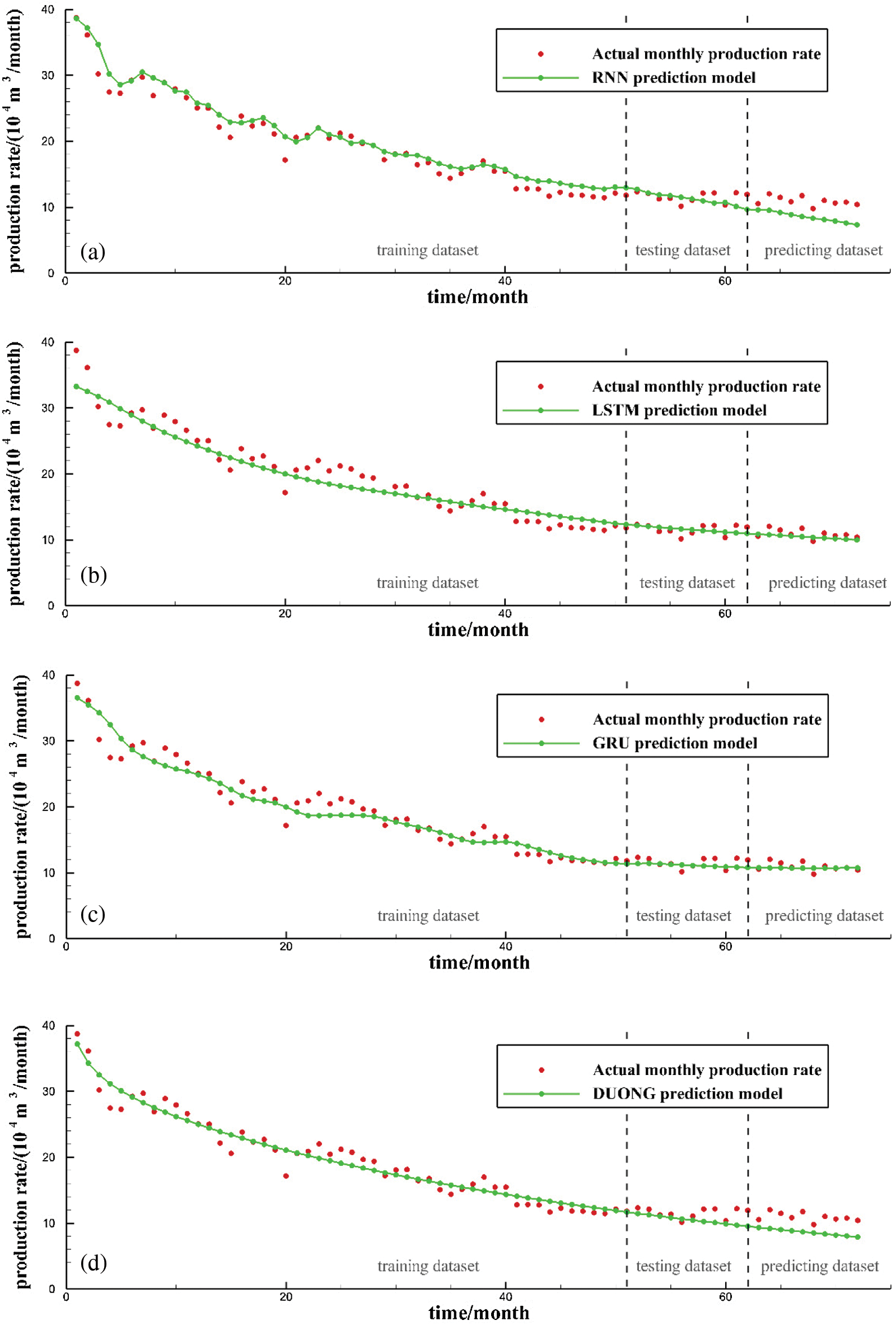
Figure 7: Production prediction performance for Well X21: (a) RNN model; (b) LSTM model; (c) GRU model; (d) Duong model
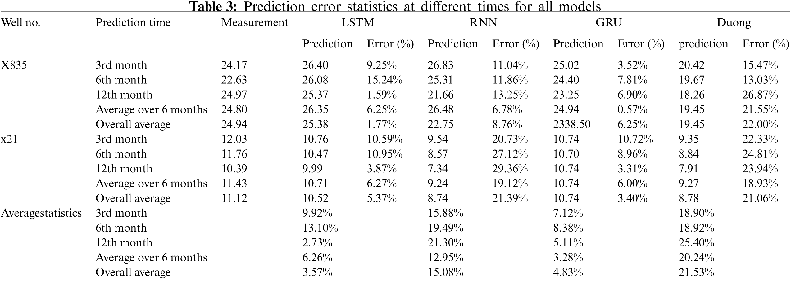
To further quantify the prediction performance of the models, Table 3 presents the prediction results of the average production of the prediction model in the third, sixth, 12th, and next six months, as well as the average production of all prediction sets. It can be seen that, in the examples of the two wells under study, the prediction results of the GRU and LSTM models are better than those of the RNN and Duong models in terms of the prediction accuracy for the tight gas production problem. In addition, by calculating the average value of the two wells, it can be shown that the GRU model exhibits slightly better performance than the LSTM model in the prediction results of average production in the third, sixth, and next six months, while the LSTM model has a better performance than the GRU model in the prediction of the average production in the 12th month and all training sets. Therefore, the predictive performance of the LSTM and GRU models is comparable.
The 13 gas wells in the tight gas field studied were further analyzed and separate predictions made using the LSTM, GRU, and RNN models. The predictive performance statistics of the three sequence learning models based on 13 tight gas production wells are plotted in Fig. 8. It is found that the average absolute percentage error of the RNN model is the largest among the three sequence learning models, and its error variance is also the largest. This means that the predictive performance of the RNN model is the least accurate. On average, the predictive error of the LSTM model is slightly lower than that of the GRU model. However, the prediction error variance of the GRU model is lower than that of the LSTM model, and the prediction error of the LSTM model is more divergent. This indicates that the predictive performance of the LSTM model may be more unstable than that of the GRU model. Despite the minor difference between the LSTM and GRU models, overall, the prediction-error distributions are very similar to each other, which means that the predictive abilities of the LSTM and GRU models are almost equally good.
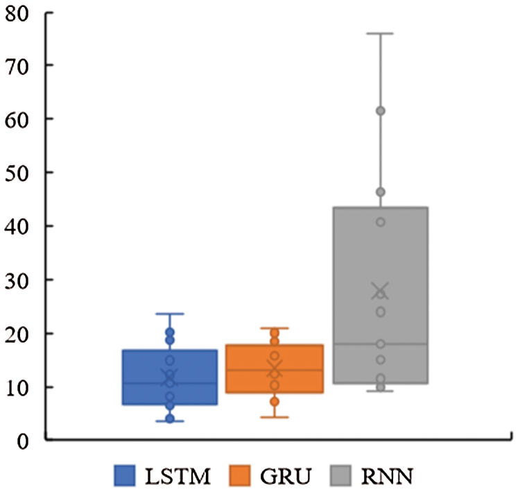
Figure 8: Predictive performance statistics based on 13 tight gas production wells
3.4 The Effect of Training Window on Prediction
The size of dataset used to train the sequence learning models need to be investigated since it can provide us the information on how many data it requires to make an accurate prediction. Figs. 6b and 6c already show production prediction results of the LSTM model and GRU model when 70% of the data is used for the training model, 15% of the dataset for the prediction. To further investigate the effect of the training window on the predictive ability of the LSTM and GRU models, the training dataset is reduced and testing dataset is increased. Fig. 9 show the production prediction results when only 50% of the data is used for training the model and 35% of the dataset for the prediction. Fig. 10 show the production prediction results 30% of the dataset is used for training the model and 55% of the dataset for the prediction.
By comparing the predicted results of Figs. 6b, 9a and 10a, when the training dataset was reduced from 70% to 50% and then to 30%, the average relative errors of LSTM model are 1.77%, 9.81% and 8.96%, respectively. It shows that with the decrease of training set and the increase of prediction time steps, the prediction error of LSTM model can still remain within the allowable range of engineering application. And the prediction error of LSTM model remains stable after increasing the prediction dataset to a certain extent. It is proved that LSTM model can capture the internal relationship between production data in a long period of time and reliable long-term predictions can be made even when the early stages of production data are available.
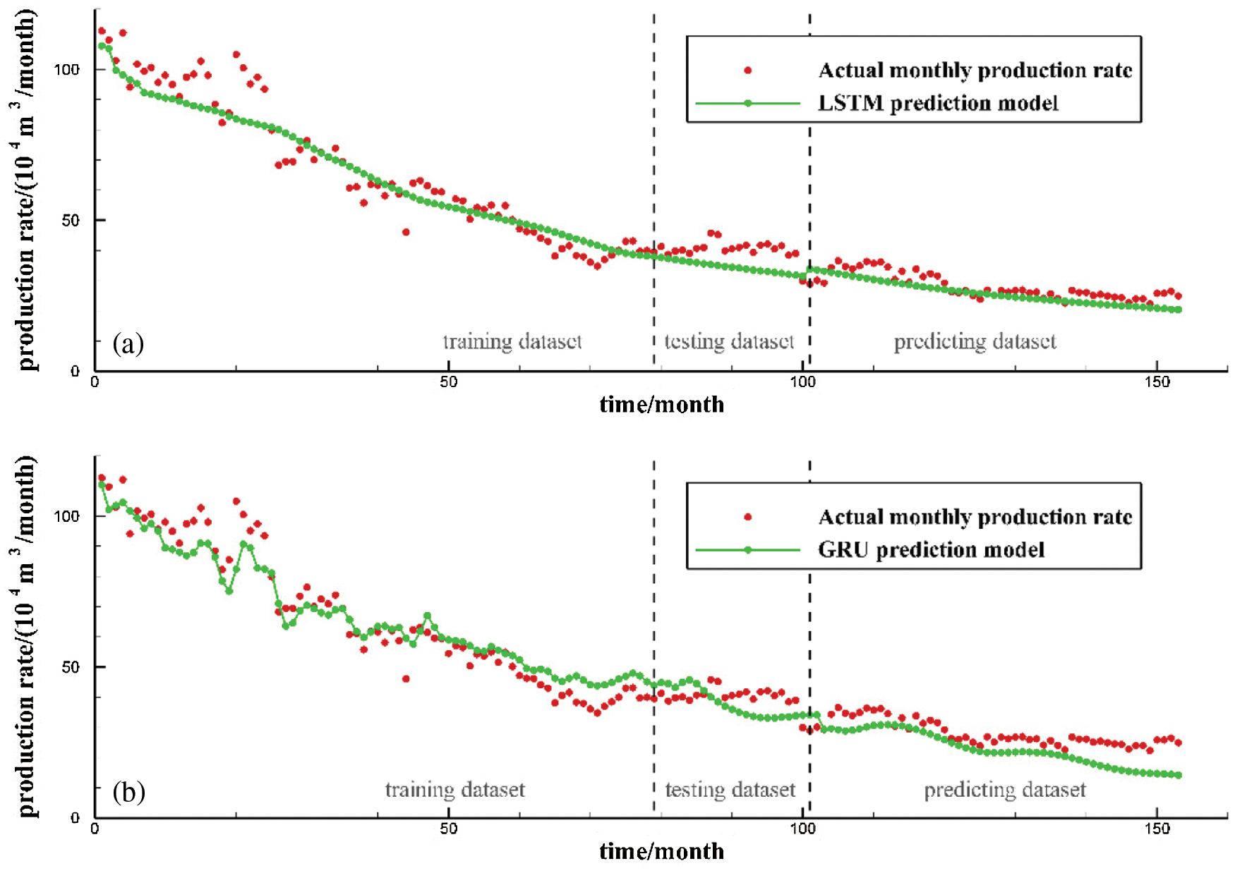
Figure 9: LSTM model and GRU model production prediction results with 50% data as training dataset and 35% data as predicting dataset: (a) LSTM model; (b) GRU model
By comparing the prediction results of Figs. 6c, 9b and 10b, when the training set was reduced from 70% to 50% and then to 30%, the average relative errors of the GRU model are 6.25%, 19.70% and 57.26%, respectively. It indicates that with the decrease of training set and the increase of prediction time steps, the prediction error of GRU model increases gradually. It shows that GRU model cannot capture the tendency of production decline accurately, and is not suitable for long-term prediction of gas well production.
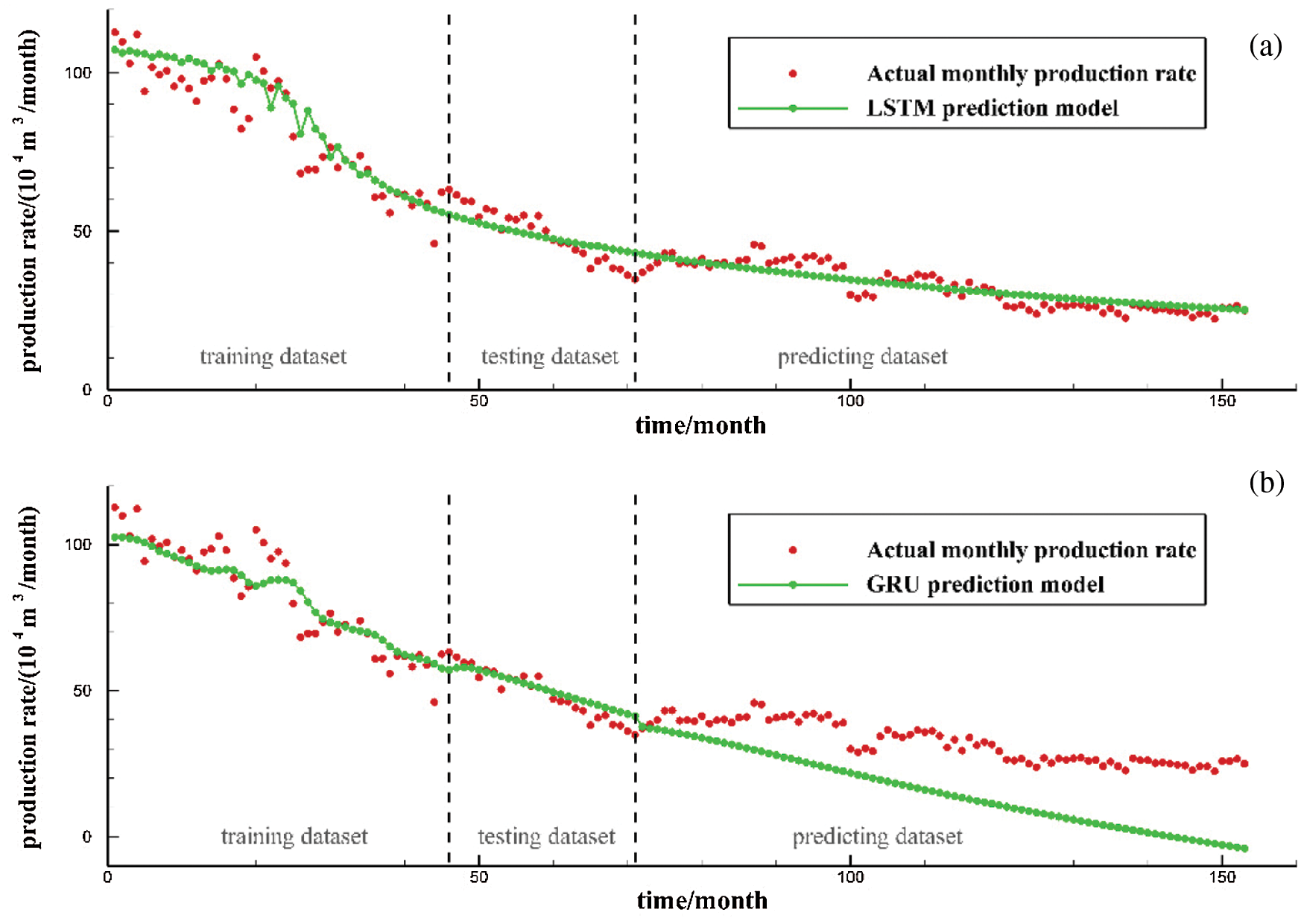
Figure 10: LSTM model and GRU model production prediction results with 30% data as training dataset and 55% data as predicting dataset: (a) LSTM model; (b) GRU model
The predictive performances of optimized sequence learning models are investigated, and the following conclusions can be drawn:
(1) The RNN, LSTM, and GRU models are three typical sequence learning models that can be used to cope with tight gas production problems in a data-driven way without the limitation of the explicit mathematical expression.
(2) The tight gas production data can be smoothed and de-noised before they are used to build the data-driven sequence learning model. The pre-processing data may not fit the well with the extreme fluctuation, but they can improve the generalization of the methods.
(3) The sequence learning models must be optimized to achieve their best performances, and the PSO method is an effective way of optimizing the hyper-parameters. The objective function of the optimization can be reduced, and the optimized objective-function values of the LSTM and GRU models are smaller than those of the RNN model due to the introduction of gate control.
(4) The optimal LSTM model has a more complex unit-cell neural network structure than the RNN and GRU models. Both the LSTM and RNN models can manage the long dependencies of the sequence data by using gates to control the information flow. The GRU model requires less time to be trained and optimized, but are suitable for short-term forecasting. LSTM has better long-term forecasting ability.
(5) The predictive performances of the three sequence learning models and Duong model studied are compared using tight gas production data. It has been shown that the predictive performances in the short-term forecasting problem of both the LSTM and GRU models are similar and are much better than that of the RNN and Duong models, the predictive performances in the long-term forecasting problem of the LSTM models are much better than that of the GRU models.
Funding Statement: This work was funded by the Joint Funds of the National Natural Science Foundation of China (U19B6003) and the PetroChina Innovation Foundation (Grant No. 2020D-5007-0203); and it was further supported by the Science Foundation of China University of Petroleum, Beijing (Nos. 2462021YXZZ010, 2462018QZDX13, and 2462020YXZZ028). We thank LetPub (https://www.letpub.com) for its linguistic assistance during the preparation of this manuscript.
Conflicts of Interest: The authors declare that they have no conflicts of interest to report regarding the present study.
1. Zou, C., Zhu, R., Liu, K., Su, L., Bai, B. et al. (2012). Tight gas sandstone reservoirs in China: Characteristics and recognition criteria. Journal of Petroleum Science and Engineering, 88, 82–91. DOI 10.1016/j.petrol.2012.02.001. [Google Scholar] [CrossRef]
2. Wang, L., Zhang, Y., Zhang, N., Zhao, C., Wu, W. (2020). Pore structure characterization and permeability estimation with a modified multimodal Thomeer pore size distribution function for carbonate reservoirs. Journal of Petroleum Science and Engineering, 193, 107426. DOI 10.1016/j.petrol.2020.107426. [Google Scholar] [CrossRef]
3. Vishkai, M., Gates, I. (2019). On multistage hydraulic fracturing in tight gas reservoirs: Montney formation, Alberta, Canada. Journal of Petroleum Science and Engineering, 174, 1127–1141. DOI 10.1016/j.petrol.2018.12.020. [Google Scholar] [CrossRef]
4. Abou-Sayed, I. S., Schueler, S., Ehrl, E., Hendricks, W. (1996). Multiple hydraulic fracture stimulation in a deep horizontal tight gas well. Journal of Petroleum Technology, 48(2), 163–168. DOI 10.2118/30532-JPT. [Google Scholar] [CrossRef]
5. Clarkson, C. R., Beierle, J. J. (2010). Integration of microseismic and other post-fracture surveillance with production analysis: A tight gas study. SPE Unconventional Gas Conference, OnePetro, Pittsburgh, Pennsylvania, USA. [Google Scholar]
6. Feng, G., Huang, Z., Yang, H. (2020). A 3D gas and water simulator considering nonlinear flow behaviors for abnormal high-pressure tight gas reservoirs. Chemistry and Technology of Fuels and Oils, 56, 60–72. DOI 10.1007/s10553-020-01111-z. [Google Scholar] [CrossRef]
7. Yao, J., Sun, H., Fan, D. Y., Wang, C. C., Sun, Z. X. (2013). Numerical simulation of gas transport mechanisms in tight shale gas reservoirs. Petroleum Science, 10(4), 528–537. DOI 10.1007/s12182-013-0304-3. [Google Scholar] [CrossRef]
8. Freeman, C. M., Moridis, G., Ilk, D., Blasingame, T. A. (2013). A numerical study of performance for tight gas and shale gas reservoir systems. Journal of Petroleum Science and Engineering, 108, 22–39. DOI 10.1016/j.petrol.2013.05.007. [Google Scholar] [CrossRef]
9. Song, H., Cao, Y., Yu, M., Wang, Y., Killough, J. E. et al. (2015). Impact of permeability heterogeneity on production characteristics in water-bearing tight gas reservoirs with threshold pressure gradient. Journal of Natural Gas Science and Engineering, 22, 172–181. DOI 10.1016/j.jngse.2014.11.028. [Google Scholar] [CrossRef]
10. Zafar, A., Su, Y. L., Li, L., Fu, J. G., Mehmood, A. et al. (2020). Tight gas production model considering TPG as a function of pore pressure, permeability and water saturation. Petroleum Science, 17(5), 1356–1369. DOI 10.1007/s12182-020-00430-4. [Google Scholar] [CrossRef]
11. Li, X. P., Cao, L. N., Luo, C., Zhang, B., Zhang, J. Q. et al. (2017). Characteristics of transient production rate performance of horizontal well in fractured tight gas reservoirs with stress-sensitivity effect. Journal of Petroleum Science and Engineering, 158, 92–106. DOI 10.1016/j.petrol.2017.08.041. [Google Scholar] [CrossRef]
12. Zhao, K., Du, P. (2019). Performance of horizontal wells in composite tight gas reservoirs considering stress sensitivity. Advances in Geo-Energy Research, 3(3), 287–303. DOI 10.26804/ager. [Google Scholar] [CrossRef]
13. Ding, X., Zhang, F., Zhang, G. (2020). Modelling of time-dependent proppant embedment and its influence on tight gas production. Journal of Natural Gas Science and Engineering, 82, 103519. DOI 10.1016/j.jngse.2020.103519. [Google Scholar] [CrossRef]
14. Panja, P., Pathak, M., Deo, M. (2019). Productions of volatile oil and gas-condensate from liquid rich shales. Advances in Geo-Energy Research, 3(1), 29–42. DOI 10.26804/ager. [Google Scholar] [CrossRef]
15. Neshat, S. S., Okuno, R., Pope, G. A. (2020). Simulation of solvent treatments for fluid blockage removal in tight formations using coupled three-phase flash and capillary pressure models. Journal of Petroleum Science and Engineering, 195, 107442. DOI 10.1016/j.petrol.2020.107442. [Google Scholar] [CrossRef]
16. Hassan, A. M., Mahmoud, M. A., Al-Majed, A. A., Al-Nakhli, A. R., Bataweel, M. A. (2019). Water blockage removal and productivity index enhancement by injecting thermochemical fluids in tight sandstone formations. Journal of Petroleum Science and Engineering, 182, 106298. DOI 10.1016/j.petrol.2019.106298. [Google Scholar] [CrossRef]
17. Wang, J., Zhou, F. J. (2021). Cause analysis and solutions of water blocking damage in cracked/non-cracked tight sandstone gas reservoirs. Petroleum Science, 18(1), 219–233. DOI 10.1007/s12182-020-00482-6. [Google Scholar] [CrossRef]
18. Zeng, J., Liu, J., Li, W., Leong, Y. K., Elsworth, D. et al. (2021). Shale gas reservoir modeling and production evaluation considering complex gas transport mechanisms and dispersed distribution of kerogen. Petroleum Science, 18(1), 195–218. DOI 10.1007/s12182-020-00495-1. [Google Scholar] [CrossRef]
19. Ru, Z., An, K., Hu, J. (2019). The impact of sulfur precipitation in developing a sour gas reservoir with pressure-sensitive effects. Advances in Geo-Energy Research, 3(3), 268–276. DOI 10.26804/ager. [Google Scholar] [CrossRef]
20. Wang, J., Yu, L., Yuan, Q. (2019). Experimental study on permeability in tight porous media considering gas adsorption and slippage effect. Fuel, 253, 561–570. DOI 10.1016/j.fuel.2019.05.048. [Google Scholar] [CrossRef]
21. Li, D., Xu, C., Wang, J. Y., Lu, D. (2014). Effect of Knudsen diffusion and Langmuir adsorption on pressure transient response in tight-and shale-gas reservoirs. Journal of Petroleum Science and Engineering, 124, 146–154. DOI 10.1016/j.petrol.2014.10.012. [Google Scholar] [CrossRef]
22. Arps, J. J. (1945). Analysis of decline curves. Transactions of the AIME, 160(1), 228–247. DOI 10.2118/945228-G. [Google Scholar] [CrossRef]
23. Robertson, S. (1988). Generalized hyperbolic equation. Society of Petroleum Engineers. [Google Scholar]
24. Ilk, D., Rushing, J. A., Perego, A. D., Blasingame, T. A. (2008). Exponential vs. hyperbolic decline in tight gas sands: Understanding the origin and implications for reserve estimates using Arps’ decline curves. SPE Annual Technical Conference and Exhibition, OnePetro, Denver, Colorado, USA. [Google Scholar]
25. Valko, P. P. (2009). Assigning value to stimulation in the barnett shale: A simultaneous analysis of 7000 plus production hystories and well completion records. SPE Hydraulic Fracturing Technology Conference, OnePetro, The Woodlands, Texas. [Google Scholar]
26. Valkó, P. P., Lee, W. J. (2010). A better way to forecast production from unconventional gas wells. in SPE Annual Technical Conference and Exhibition, Society of Petroleum Engineers, Florence, Italy. [Google Scholar]
27. D Duong, A. N. (2010, October). An unconventional rate decline approach for tight and fracture-dominated gas wells. Canadian Unconventional Resources and International Petroleum Conference, OnePetro, Calgary, Alberta, Canada. [Google Scholar]
28. Wang, S., Chen, S. (2019). Insights to fracture stimulation design in unconventional reservoirs based on machine learning modeling. Journal of Petroleum Science and Engineering, 174, 682–695. DOI 10.1016/j.petrol.2018.11.076. [Google Scholar] [CrossRef]
29. Luo, G., Tian, Y., Bychina, M., Ehlig-Economides, C. (2018). Production optimization using machine learning in Bakken shale. Unconventional Resources Technology Conference, pp. 2174–2197. Society of Exploration Geophysicists, American Association of Petroleum Geologists, Society of Petroleum Engineers, Houston, Texas, USA. [Google Scholar]
30. Noshi, C. I., Eissa, M. R., Abdalla, R. M., (2019). An intelligent data driven approach for production prediction. Offshore Technology Conference, OnePetro, Houston, Texas. [Google Scholar]
31. Li, X., Chan, C. W., Nguyen, H. H. (2013). Application of the neural decision tree approach for prediction of petroleum production. Journal of Petroleum Science and Engineering, 104, 11–16. DOI 10.1016/j.petrol.2013.03.018. [Google Scholar] [CrossRef]
32. Wang, S., Chen, Z., Chen, S. (2019). Applicability of deep neural networks on production forecasting in bakken shale reservoirs. Journal of Petroleum Science and Engineering, 179, 112–125. DOI 10.1016/j.petrol.2019.04.016. [Google Scholar] [CrossRef]
33. Tian, C., Horne, R. N. (2019). Applying machine-learning techniques to interpret flow-rate, pressure, and temperature data from permanent downhole gauges. SPE Reservoir Evaluation & Engineering, 22(2), 386–401. DOI 10.2118/174034-PA. [Google Scholar] [CrossRef]
34. Sun, J., Ma, X., Kazi, M. (2018). Comparison of decline curve analysis DCA with recursive neural networks RNN for production forecast of multiple wells. SPE Western Regional Meeting, OnePetro, Garden Grove, California, USA. [Google Scholar]
35. Zhang, D., Chen, Y. T., Meng, J. (2018). Synthetic well logs generation via recurrent neural networks. Petroleum Exploration and Development, 45(4), 629–639. DOI 10.1016/S1876-3804(18)30068-5. [Google Scholar] [CrossRef]
36. Song, X., Liu, Y., Xue, L., Wang, J., Zhang, J. et al. (2020). Time-series well performance prediction based on long short-term memory (LSTM) neural network model. Journal of Petroleum Science and Engineering, 186, 106682. DOI 10.1016/j.petrol.2019.106682. [Google Scholar] [CrossRef]
37. Li, X., Ma, X., Xiao, F., Wang, F., Zhang, S. (2020). Application of gated recurrent unit (GRU) neural network for smart batch production prediction. Energies, 13(22), 6121. DOI 10.3390/en13226121. [Google Scholar] [CrossRef]
38. Hopfield, J. J. (1982). Neural networks and physical systems with emergent collective computational abilities. Proceedings of the National Academy of Sciences, 79(8), 2554–2558. DOI 10.1073/pnas.79.8.2554. [Google Scholar] [CrossRef]
39. Werbos, P. J. (1990). Backpropagation through time: What it does and how to do it. Proceedings of the IEEE, 78(10), 1550–1560. DOI 10.1109/5.58337. [Google Scholar] [CrossRef]
40. Bengio, Y., Simard, P., Frasconi, P. (1994). Learning long-term dependencies with gradient descent is difficult. IEEE Transactions on Neural Networks, 5(2), 157–166. DOI 10.1109/TNN.72. [Google Scholar] [CrossRef]
41. Hochreiter, S., Bengio, Y., Frasconi, P., Schmidhuber, J. (2001). Gradient flow in recurrent nets: The difficulty of learning long-term dependencies. A Field Guide to Dynamical Recurrent Networks, IEEE, pp. 237--243, DOI 10.1109/9780470544037.ch14. [Google Scholar] [CrossRef]
42. Hochreiter, S., Schmidhuber, J. (1997). Long short-term memory. Neural Computation, 9(8), 1735–1780. DOI 10.1162/neco.1997.9.8.1735. [Google Scholar] [CrossRef]
43. Cho, K., van Merriënboer, B., Bahdanau, D., Bengio, Y. (2014). On the properties of neural machine translation: Encoder-decoder approaches. Proceedings of SSST-8, Eighth Workshop on Syntax, Semantics and Structure in Statistical Translation. DOI 10.3115/v1/W14-4012. [Google Scholar] [CrossRef]
44. Chung, J., Gulcehre, C., Cho, K., Bengio, Y. (2014). Empirical evaluation of gated recurrent neural networks on sequence modeling. arXiv preprint arXiv:1412.3555. [Google Scholar]
45. Savitzky, A., Golay, M. J. (1964). Smoothing and differentiation of data by simplified least squares procedures. Analytical Chemistry, 36(8), 1627–1639. DOI 10.1021/ac60214a047. [Google Scholar] [CrossRef]
46. Luo, J., Ying, K., Bai, J. (2005). Savitzky–Golay smoothing and differentiation filter for even number data. Signal Processing, 85(7), 1429–1434. DOI 10.1016/j.sigpro.2005.02.002. [Google Scholar] [CrossRef]
47. Yu, S. (2013). Best practice of using empirical methods for production forecast and EUR estimation in tight/shale gas reservoirs. SPE Unconventional Resources Conference Canada, Society of Petroleum Engineers, Calgary, Alberta, Canada. [Google Scholar]
48. Wilson, A. (2015). Comparison of empirical and analytical methods for production forecasting. Journal of Petroleum Technology, 67(4), 133–136. DOI 10.2118/0415-0133-JPT. [Google Scholar] [CrossRef]
 | This work is licensed under a Creative Commons Attribution 4.0 International License, which permits unrestricted use, distribution, and reproduction in any medium, provided the original work is properly cited. |