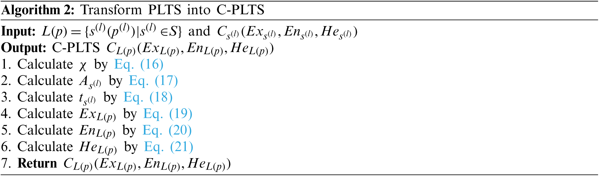
| Computer Modeling in Engineering & Sciences |
DOI: 10.32604/cmes.2022.019501
ARTICLE
A Personalized Comprehensive Cloud-Based Method for Heterogeneous MAGDM and Application in COVID-19
School of Information Management, Jiangxi University of Finance and Economics, Nanchang, 330013, China
*Corresponding Author: Shuping Wan. Email: shupingwan@163.com
Received: 27 September 2021; Accepted: 30 November 2021
Abstract: This paper proposes a personalized comprehensive cloud-based method for heterogeneous multi-attribute group decision-making (MAGDM), in which the evaluations of alternatives on attributes are represented by LTs (linguistic terms), PLTSs (probabilistic linguistic term sets) and LHFSs (linguistic hesitant fuzzy sets). As an effective tool to describe LTs, cloud model is used to quantify the qualitative evaluations. Firstly, the regulation parameters of entropy and hyper entropy are defined, and they are further incorporated into the transformation process from LTs to clouds for reflecting the different personalities of decision-makers (DMs). To tackle the evaluation information in the form of PLTSs and LHFSs, PLTS and LHFS are transformed into comprehensive cloud of PLTS (C-PLTS) and comprehensive cloud of LHFS (C-LHFS), respectively. Moreover, DMs’ weights are calculated based on the regulation parameters of entropy and hyper entropy. Next, we put forward cloud almost stochastic dominance (CASD) relationship and CASD degree to compare clouds. In addition, by considering three perspectives, a comprehensive tri-objective programing model is constructed to determine the attribute weights. Thereby, a personalized comprehensive cloud-based method is put forward for heterogeneous MAGDM. The validity of the proposed method is demonstrated with a site selection example of emergency medical waste disposal in COVID-19. Finally, sensitivity and comparison analyses are provided to show the effectiveness, stability, flexibility and superiorities of the proposed method.
Keywords: Heterogeneous MAGDM; regulation parameter; C-PLTS; C-LHFS; CASD
Multi-attribute group decision-making (MAGDM) refers to a decision situation where a group of decision-makers (DMs) provide their own opinions on a given set of alternatives under a set of attributes, and then select the optimal alternative(s) by aggregating their opinions [1–6]. Since the real-life MAGDM problems often involve multiple different types of attributes, it is not easy for DMs to evaluate all attributes in only one form of evaluation information, which results in the appearance of heterogeneous MAGDM. In heterogeneous MAGDM process, the evaluations of different attributes can be expressed by qualitative and quantitative forms. For example, when a customer selects a car, a real number or an interval number can be used to evaluate its price, but a LT (linguistic term) or its extended forms will be preferred than quantitative value to evaluate its safety. Due to the growing uncertainty of actual decision-making environments, it is more convenient and flexible for DMs to employ qualitative forms, e.g., LT, PLTS (probabilistic linguistic term set), LHFS (linguistic hesitant fuzzy set), to characterize the evaluation information of alternatives on attributes. Both PLTS and LHFS are two important extensions of LT. PLTS, proposed by Pang et al. [7], consists of LTs and their corresponding probabilities. LHFS, initiated by Meng et al. [8], contains LTs and their corresponding memberships. For example, a group of DMs are invited to select a site for emergency medical waste disposal during the outbreak of COVID-19. Five attributes, i.e., geographical location, equipment, process technologies, disposal capacity and transport capacity, are chosen to evaluate the alternatives. LTs are suitable to evaluate the geographical location. Since the evaluations for equipment and process technologies are divided into two parts: LTs and corresponding probabilities, PLTSs are suitable to evaluate the equipment and process technologies. Besides, it is easy for DMs to evaluate the disposal capacity and the transportation capacity by using LHFSs. Therefore, the site selection of emergency medical waste disposal is a typical problem of heterogeneous MAGDM with different types of qualitative evaluations. Currently, many scholars have studied heterogeneous MAGDM problems. Yu et al. [1] developed a fusion method based on trust and behavior analysis for heterogeneous MAGDM scenarios. Liu et al. [9] proposed a new axiomatic design-based mathematical programming method for heterogeneous MAGDM with linguistic fuzzy truth degrees. Gao et al. [10] provided a consensus model for heterogeneous MAGDM with several attribute sets. Wan et al. [11] initiated a new prospect theory based method for heterogeneous MAGDM with hybrid fuzzy truth degrees of alternative comparisons. With the in-depth study of previous literature, many heterogeneous MAGDM problems have been effectively solved. However, there is little research on heterogeneous MAGDM with multiple qualitative forms (especially LT, PLTS and LHFS). To fill the gap, this paper intends to use LTs, PLTSs and LHFSs to portray heterogeneous evaluations.
Qualitative evaluations are not easy to be computed directly, especially when DMs use diverse forms of qualitative evaluations. At present, some models have been developed to deal with the calculations of qualitative evaluations, such as linguistic symbolic model [12], two-tuple linguistic model [13], cloud model [14,15]. Linguistic symbolic model and two-tuple linguistic model deal with LTs by converting them into real numbers. Cloud model proposed by Li et al. [14,15] is a more effective tool to describe qualitative concepts since it has strong power in capturing the fuzziness and randomness of LTs, simultaneously. Based on the probability theory and fuzzy set theory, the cloud model utilizes three numerical characteristics, i.e., mathematical expectation
Although the above mentioned cloud-based methods [22–32] are efficient in handing various practical decision-making problems, there still exist some defects as follows:
(1) Some previous studies [22–27,29,31,32] depicted the evaluations only with a single qualitative form, which might limit their applications in practical decision-making problems.
(2) Few studies took DMs’ personalities into account during the transformation process. Wang et al. [24] introduced overlap parameter into the transformation process to reflect the DMs’ personality and preference. But the determination of overlap parameter is a little subjective, which may lead to unreasonable decision results.
(3) The comprehensive clouds in existing approaches [23,32] may cause the loss and distortion of evaluation information.
(4) Methods in [22,24,26,29,32] used the expected score values of clouds to rank the alternatives, while methods in [23,27,30,33,34] utilized the closeness coefficient and priority vector to rank the alternatives. However, the expected score values of clouds sometimes are unstable since the expected score values are generated randomly. The closeness coefficient and priority vector depend on the distances between clouds, but different definitions of distance between clouds usually generate different ranking results.
To overcome the above limitations, this paper develops a personalized comprehensive cloud-based method for heterogeneous MAGDM, in which the evaluations of alternatives on attributes are represented as LTs, PLTSs and LHFSs. Regulation parameters of entropy and hyper entropy are proposed to reflect the DMs’ personalities. Two approaches are put forward to transform PLTS and LHFS into comprehensive cloud of PLTS (C-PLTS) and comprehensive cloud of LHFS (C-LHFS), respectively. The cloud almost stochastic dominance (CASD) relationship and CASD degree are initiated to compare clouds and further rank the alternatives. In addition, a novel approach is presented to obtain DMs’ weights and a comprehensive tri-objective programing model is constructed to determine the attribute weights. The proposed method is employed to the site selection of emergency medical waste disposal in COVID-19. Compared with existing studies, the major contributions of this paper are highlighted in the following four aspects:
(1) Regulation parameters of entropy and hyper entropy are defined objectively. By incorporating regulation parameters into the transformation process, DMs’ personalities are reflected well. Moreover, DMs’ weights are objectively determined based on the proposed regulation parameters.
(2) From the perspectives of probability and membership degree, two approaches are put forward to transform PLTS and LHFS into C-PLTS and C-LHFS, respectively. The modified ratios of LTs decrease the loss and distortion of evaluation information.
(3) CASD relationship and CASD degree are defined and used to compare clouds. Based on the proposed comparison approach for clouds, the alternatives are ranked and the ranking results are stable and effective.
(4) A comprehensive tri-objective programing model is constructed to determine the attribute weights. In this model, three perspectives are considered, including differentiation between evaluation values, relationship between attributes and the amount of information contained in evaluation values. The setting of balance coefficients enables DMs to make a tradeoff in the three perspectives, which can improve the flexibility of the proposed method.
The remainder of this paper is organized as follows: Section 2 briefly introduces some concepts related to LTs and reviews cloud model as well as almost first-degree stochastic dominance (AFSD). Section 3 describes the heterogeneous MAGDM problem and develops two novel transformation approaches from PLTS and LHFS to comprehensive clouds. In Section 4, a personalized comprehensive cloud-based method is proposed for heterogeneous MAGDM problem. A numerical example and sensitivity analyses are conducted to illustrate the proposed method in Section 5. Section 6 performs some comparison analyses to explain the superiorities of the proposed method. Some conclusions are summarized in Section 7.
This section briefly introduces some concepts related to LTs and reviews cloud model as well as AFSD.
2.1 LT and Some Related Concepts
Let
(i) Ordered set:
(ii) Negation operation:
In linguistic evaluation scales, the absolute deviation of semantics between any two adjacent LTs may increase, decrease or remain unchanged with increasing linguistic subscripts. To reflect various semantics deviation, linguistic scale functions (LSFs) [22] are used to flexibly portray evaluation scales according to specific semantic situations.
Definition 1. [22,36] Let
where
Three kinds of LSFs are shown below:
In LFS1, the absolute deviation between adjacent LTs remains unchanged with increasing linguistic subscripts. Take
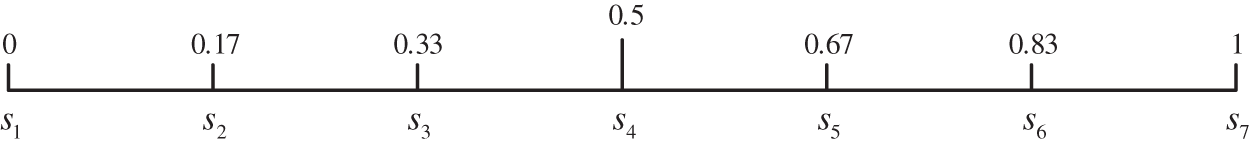
Figure 1: LSF1 (
Lots of experimental studies [37] have illustrated that a generally lies in the interval
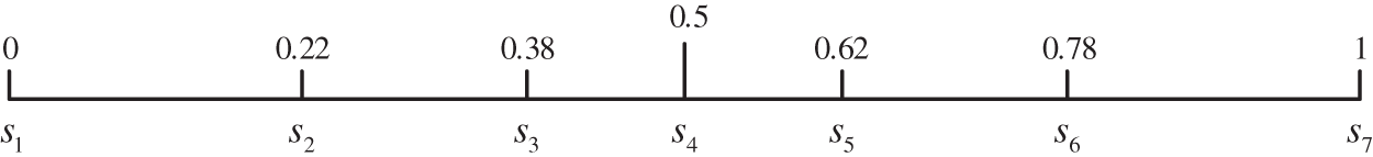
Figure 2: LSF2 (
LSF3 is defined based on prospect theory's value function and the DMs’ different sensation for the absolute deviation between adjacent linguistic subscripts.
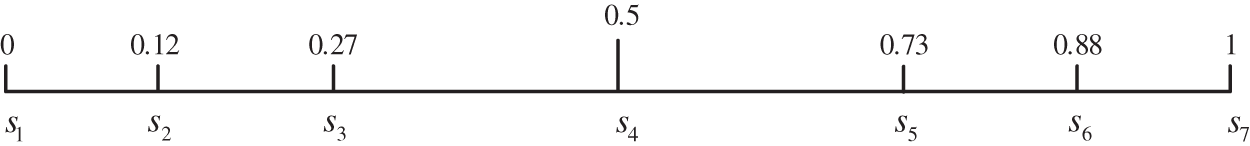
Figure 3: LSF3 (
In order to save all of the given information and facilitate calculation, the aforesaid functions can be extended into
Definition 2. [7] Let
In this paper, it is assumed that all PLTSs have already been normalized.
Definition 3. [8] Let
Definition 4. [14] Let U be the universe of discourse and T be a qualitative concept in U. If
For simplicity, normal cloud is called as cloud hereafter. The degree of certainty of x belonging to concept T is a probability distribution rather than a fixed number. Hence,
There are two kinds of uncertainty: randomness and fuzziness. Randomness refers to the uncertainty contained in an event that has a clear definition but do not necessarily occur. Fuzziness refers to the uncertainty contained in an event that has appeared but it is difficult to define it accurately [39]. There is a practical demand to describe fuzziness and randomness inherent in LTs simultaneously. Cloud can perfectly depict the overall quantitative properties of a concept through three numerical characteristics: mathematical expectation
Definition 5. [15] Given two clouds
(1)
(2)
(3)
The AFSD is used to compare two stochastic variables. It was proposed by Leshno and Levy [41]. Let
Definition 6. [41,42] For
3 Heterogeneous MAGDM Problem and Comprehensive Cloud
This section describes the heterogeneous MAGDM problem and introduces the improved transformation approach between LT and cloud in detail. Particularly, we developed two novel transformation approaches from PLTS and LHFS to comprehensive clouds.
3.1 Description for Heterogeneous MAGDM Problem
A heterogeneous MAGDM problem is to find the best solution from all feasible alternatives assessed on multiple attributes by a group of DMs. The evaluation attributes in heterogeneous MAGDM can be classed into several subsets which are expressed by different kinds of forms.
For a heterogeneous MAGDM problem, suppose that DMs
Let
3.2 Transformation between LT and Cloud
Generally, two kinds of approaches have been proposed for transformation from LTs to clouds so far. One is based on the golden radio [44], and the other is based on the LSF [22]. Wang et al. [24] introduced a parameter named overlapping degree into the transformation approach [22] to determining the degree of overlap between two adjacent clouds. With the parameter
Let
3.2.1 Determination of the Regulation Parameter of Entropy
Entropy
Definition 7. For a heterogeneous MAGDM, the average number of LTs used by DM
It is obvious that
Definition 8. The hesitant degree of DM
Obviously,
The determination of DM's hesitant degree is based on the average number of LTs that DM uses at a single evaluation in the form of PLTSs or LHFSs.
A great deal of experimental research has demonstrated that regulation parameter
Definition 9. Let
where
In the following, an example is given to illustrate how to determine the value of
Example 1. Let
Calculate the average number of LTs used by DM
Calculate the hesitant degree of DM
Then, the value of
3.2.2 Determination of the Regulation Parameter of Hyper Entropy
Hyper entropy
Definition 10. [45] The information entropy of
where z is a constant that is set to 1.28 in this paper as [45] sets. It is easily seen that
Definition 11. The information entropy of DM
where z is a constant that is set to 1.28 in this paper as [45] sets. Obviously,
The closer the memberships for corresponding LTs are to 0, the larger indeterminacy degree DMs have for corresponding LT.
Definition 12. The indeterminacy degree of
Clearly, it holds that
Definition 13. The indeterminacy degree of DM
It is easily seen that
Definition 14. Let
where
Take
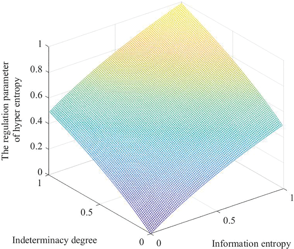
Figure 4: Graphical representation for the regulation parameter of hyper entropy (
Example 2. Following Example 1, the value of
Calculate the information entropy of each evaluation in the form of PLTSs by Eq. (8):
Calculate the information entropy of DM
Calculate the indeterminacy degree of each evaluation in the form of LHFSs by Eq. (10):
Calculate the indeterminacy degree of DM
Then, the value of
3.2.3 Specific Procedures for Transformation between LT and Cloud
Definition 15. [46] Let
Then, the specific transformation procedures are shown as follows:
(1) Calculate
Determination approaches for
(2) Calculate
Map
LSF2 Eq. (2) is adopted in this paper, where
(3) Calculate
(4) Calculate
Let
where
(5) Calculate
Based on the above analyses, the corresponding cloud for LT
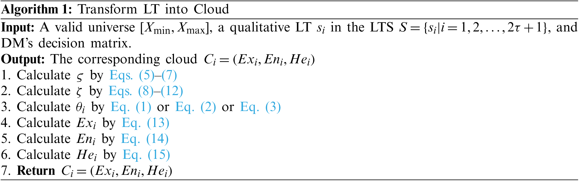
To illustrate the advantages of regulation parameters, an example is given below.
Example 3. Given a universe
Based on Eqs. (5)–(12), the regulation parameters
Based on Eqs. (2) and (13)–(15),
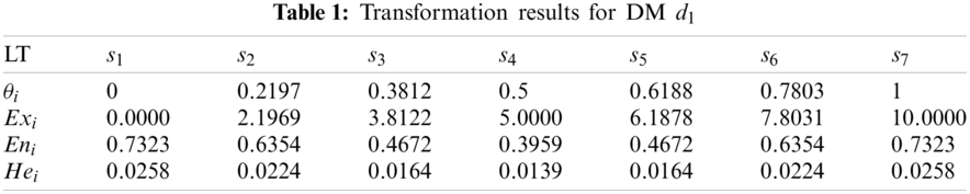
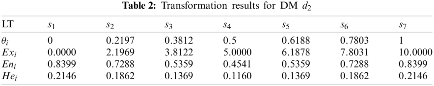
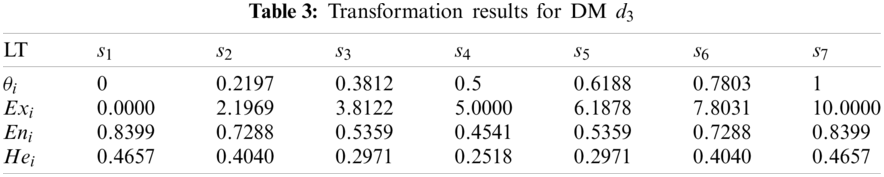
Three sets of cloud generated by DMs
It can be seen from Figs. 5–7 that the cloud drops distribution varies in width and thickness for different DMs. In previous studies [22,23,25–31,46], clouds for the corresponding LTS are usually the same for all DMs. However, since different DMs have different personalities, knowledge and experience, the width and thickness of clouds for the corresponding LTS should be different for different DMs. The more sure, confident and decisive the DM is for its evaluation matrix, the more concentrated and thinner the cloud distribution should be, vice versa. Unfortunately, most previous studies failed to notice this characteristic, whereas this paper sufficiently takes this characteristic into account. Although the overlap degree is considered in [24] to obtain personalized cloud sets for DMs, the determination of overlap degree depends on DMs’ subjective intuition. This defect is overcome in this paper. The regulation parameters are determined according to the evaluation matrix given by DM, which means the determination of regulation parameters is objective and logical.
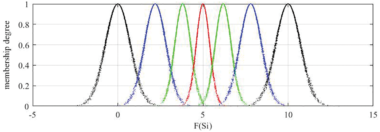
Figure 5: Clouds for the LTs used by
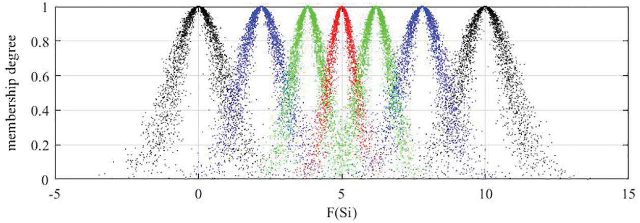
Figure 6: Clouds for the LTs used by
Figure 7: Clouds for the LTs used by
3.3 Transformation from PLTS and LHFS to Comprehensive Clouds
In this sub-section, two approaches are brought forward to transform PLTS and LHFS into comprehensive clouds, respectively.
3.3.1 Transformation from PLTS to Comprehensive Cloud
Definition 16. Let
Definition 17. [24] Given a cloud
In this paper,
The specific procedures to determine
(1) Let
(2) Use Eq. (17) to calculate the area for the PDFC of
If
(3) The modified ratio of
(4) According to Definition 5, three numerical characteristics
Based on the above analyses, the comprehensive cloud of PLTS
Example 4. Given a LTS
(1) Based on Eq. (16), the abscissa value of the intersection point
Let
(2) Based on Eq. (17), the area for the PDFC of
(3) Based on Eq. (18), the modified ratios of
(4) Based on Eqs. (19)–(21), three numerical characteristics are obtained:
Finally, the C-PLTS of
The PDFCs and 5000 cloud drops of
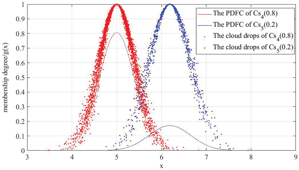
Figure 8: PDFCs and 5000 cloud drops of
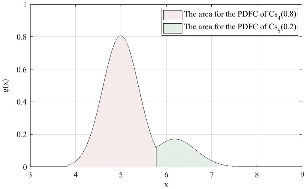
Figure 9: Areas for the PDFCs of
From
3.3.2 Transformation from LHFS to Comprehensive Cloud
Definition 18. Let
The specific procedures to determine
(1) Let
(2) Use Eq. (23) to calculate the area for the NC of
If
(3) The modified ratio of
(4) According to Definition 5, three numerical characteristics
Based on the above analyses, the comprehensive cloud of LHFS
Example 5. Given a LTS
(1) Based on Eq. (22), the abscissa value of the intersection point
Let
(2) Based on Eq. (23), the area for the NC of
(3) Based on Eq. (24), the modified ratios of
(4) Based on Eqs. (25)–(27), three numerical characteristics are obtained:
Finally, the C-LHFS of
The NCs and 5000 cloud drops of
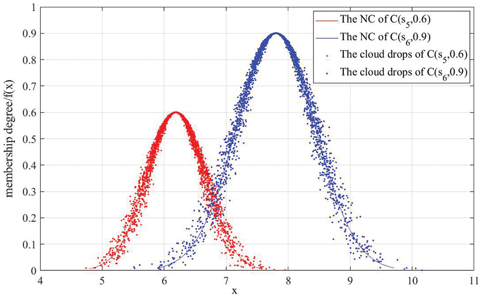
Figure 10: NCs and 5000 cloud drops of
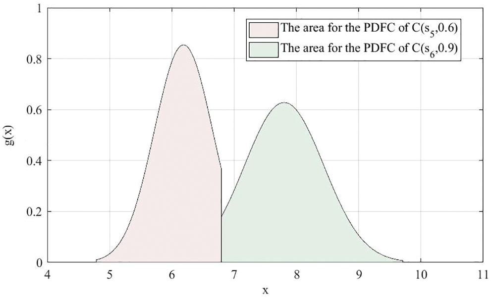
Figure 11: Areas for the PDFCs of
From
Up till now, heterogeneous MAGDM matrices in which attribute values are expressed with LTs, PLTSs and LHFSs can be transformed into homogeneous MAGDM cloud matrices. For simplicity, homogeneous MAGDM cloud matrix is called as cloud matrix hereafter. Then, the individual cloud matrix
4 Cloud-Based Heterogeneous MAGDM
In this section, some related techniques are introduced, such as the comparison approach for clouds, the determination approaches of DM weight vector and attribute weight vector. Significantly, a personalized comprehensive cloud-based method for heterogeneous MAGDM problem is proposed.
4.1 Determination of DM Weight Vector
As mentioned above, the regulation parameter
Solving Eq. (29), the DM weight vector
Example 6. Following Example 3,
By Eq. (29), the DM weight vector
Definition 19. [22] Assume that
where
Based on Eqs. (29) and (30) and basic operations of clouds in Definition 5, the individual cloud matrices
4.2 Pairwise Comparisons of Clouds
The evaluations from DMs have been transformed to clouds. As mentioned above, if
According to the characteristics of cloud, AFSD theory is used to compare the dominance relationship between clouds with characteristics
Definition 20. Let
If
As mentioned above, the CASD relationship is adapted to compare two clouds. However, this relationship cannot quantify the degree for one cloud over another. To quantify the dominance degree, CASD degree is put forward.
Let
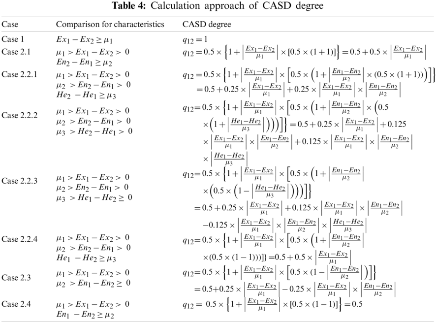
To rank the alternatives and select the optimal alternative, the comparison approach for clouds is applied to the collective cloud matrix. Alternatives
Based on the comparison approach mentioned above, the CASD degree for the alternatives
Let
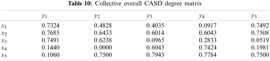
Then, the collective overall CASD degree matrix
4.3 Determination of Attribute Weight Vector
As mentioned in Section 3.1, the attribute weight vector is denoted by
4.3.1 From the Perspective of Differentiation between Evaluation Values
Let
Next, let
According to maximizing deviation approach [47], an attribute with a larger deviation value among alternatives should be assigned a larger weight, and vice versa. Thus, Model 1 is constructed as follows:
Model 1
4.3.2 From the Perspective of Relationship between Attributes
Let
Then, let
From the perspective of correlation coefficient [48], larger
Model 2
4.3.3 From the Perspective of the Amount of Information Contained in Evaluation Values
Let
It has been mentioned in Section 3.2.2 that information entropy is an important tool to measure the uncertainty of the evaluation information. It is easily known that if the information entropy of evaluations on attribute
Model 3
4.3.4 A Comprehensive Tri-Objective Optimization Model
Combining Eqs. (39)–(41), a comprehensive tri-objective optimization model is built as
To solve the comprehensive tri-objective optimization model, we add three balance coefficients
Model 4 {
} where
To solve Eq. (43), a Lagrange function is constructed as
where
The global optimal solution can be derived by taking partial derivatives of
By solving Eqs. (45) and (46), the solution can be obtained
After normalizing
Model 4 enables DMs to make a tradeoff in the above three aspects. Multifaceted considerations enhance the stability of the proposed method and the setting of balance coefficients improves the flexibility of the proposed method.
4.4 Obtaining the Ranking of Alternatives
Up till now, the collective overall CASD degree matrix
Based on the values of
4.5 Decision Steps for the Personalized Comprehensive Cloud-Based Method
A personalized comprehensive cloud-based method for heterogeneous MAGDM problem is proposed in this sub-section. Particularly, the resolution procedures of the proposed method are depicted in Fig. 12.
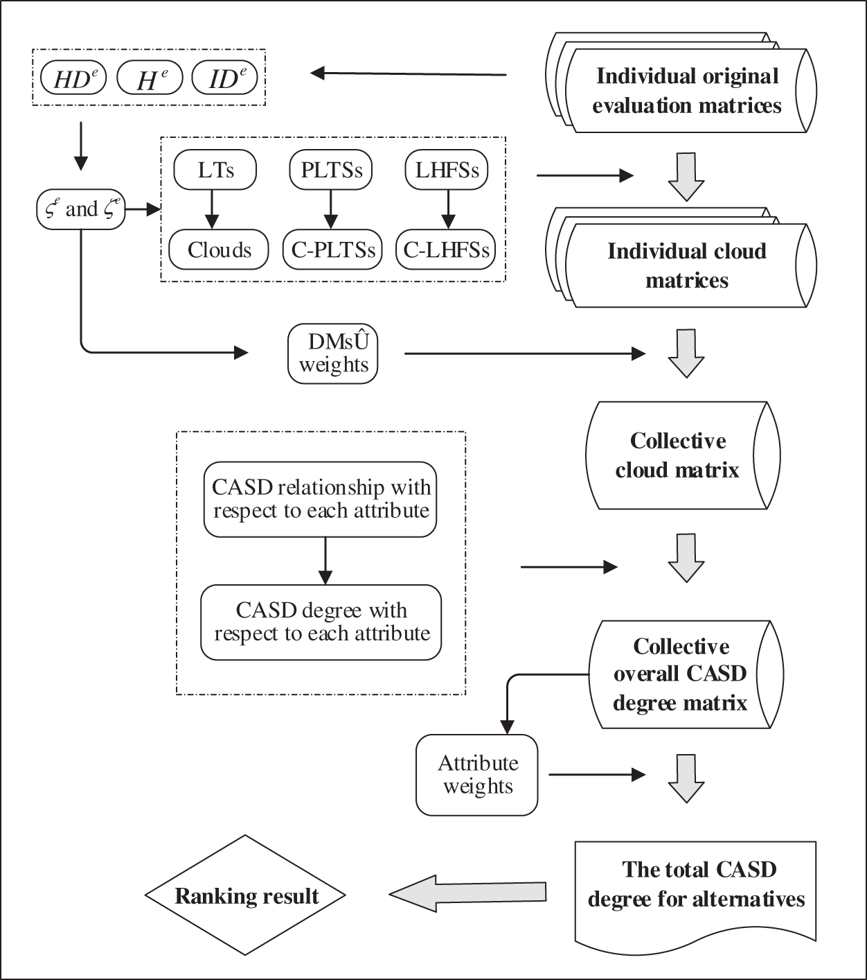
Figure 12: Resolution procedures of the proposed method
As depicted in Fig. 12, the proposed method mainly includes five steps below:
Step 1. Construct the individual original normalized evaluation matrix
DMs identify the feasible alternatives
Step 2. Transform the individual original normalized evaluation matrix
Hesitant degree
Step 3. Aggregate the individual cloud matrices
Based on Eq. (29), DM weight vector
Step 4. Transform the collective cloud matrix
Firstly, pairwise comparisons are made to judge the CASD relationships for alternatives
Step 5. Generate the ranking order of all alternatives
Set the balance coefficients
In this section, the proposed method is applied to an example of emergency medical waste disposal site selection in COVID-19. Furthermore, sensitivity analyses are conduced to demonstrate the stability and flexibility of the proposed method.
5.1 Illustration of the Proposed Method
At the end of 2019, COVID-19 broke out in various provinces and cities in China. The amount of medical waste kept rising along with the number of confirmed cases. The explosive growth of medical waste occurred in many cities, and the lack of disposal capacity made the situation more serious. In such an emergency situation, medical waste disposal becomes a special battlefield in the fight against pneumonia. If these massive amounts of medical waste that may carry the virus were not disposed in a safe and timely way, it was likely to cause secondary infections and further spread of COVID-19, which may result in a series of unimaginable aftermaths. Generally, qualified medical waste disposal companies existed previously were completely at full capacity in many cities during the outbreak of COVID-19. In order to cope with the increasing amount of medical waste, many local governments adopted a series of emergency measures. One of these measures was converting other waste disposal companies, such as industrial hazardous waste disposal companies and solid waste disposal companies, to medical waste disposal sites temporarily for emergency disposal of medical waste. The selection for emergency medical waste disposal sites can be regarded as a heterogeneous MAGDM problem.
To select a suitable emergency medical waste disposal site from five alternatives
5.1.2 Resolution Process by Using the Proposed Method of This Paper
The procedures are summarized in the following steps:
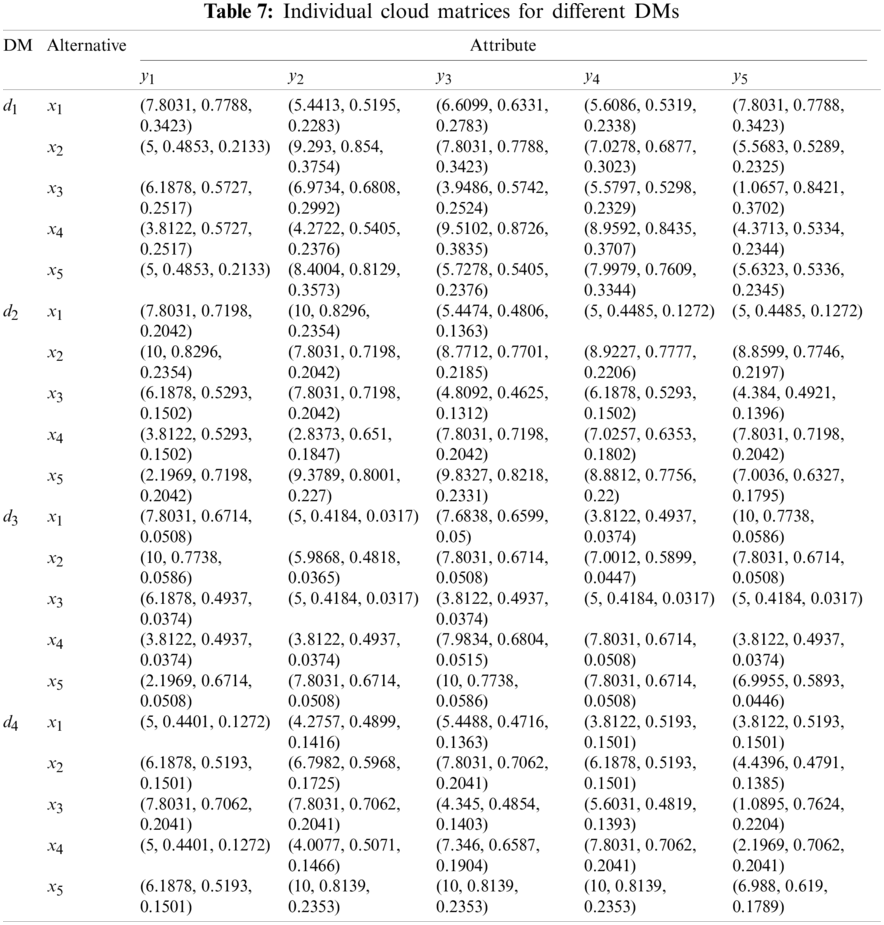
Step 1. The individual original normalized evaluation matrices
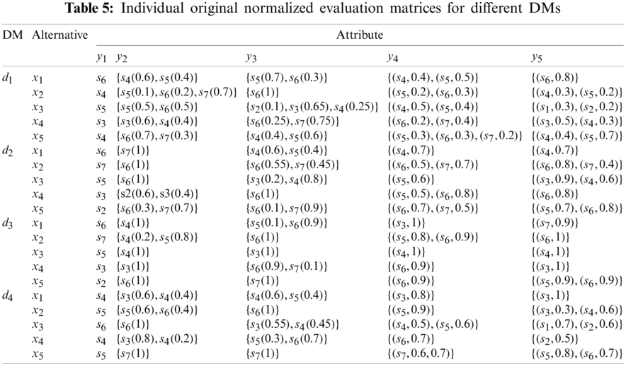
Step 2. Based on Eqs. (5)–(12), Hesitant degree
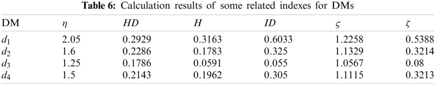
According to the proposed transformation approaches from LTs, PLTSs and LHFSs to clouds, C-PLTSs and C-LHFSs, the individual original normalized evaluation matrices
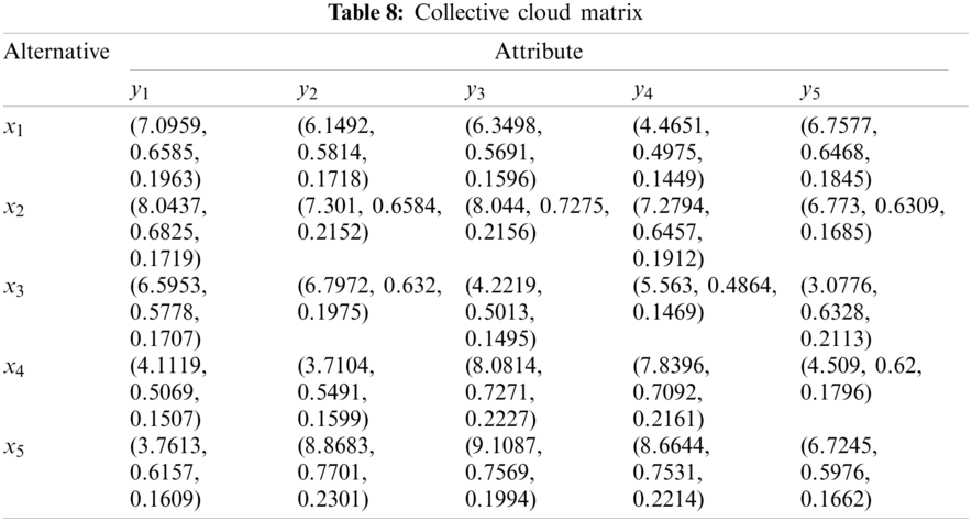
Step 3. DMs’ weights are calculated by Eq. (29). With basic operations of clouds, CWAA operator, and DM weight vector
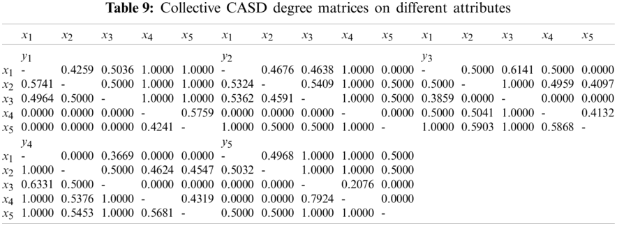
Step 4. Compare the alternatives
Step 5. Balance coefficients
With the obtained attribute weight vector, the total CASD degrees of
Thus, the ranking order is
LSFs are strictly monotonously increasing with respect to the subscript i. In linguistic evaluation scales, the absolute deviation of semantics between any two adjacent LTs may increase, decrease or remain unchanged with increasing linguistic subscripts. DMs can choose different LSFs according to the actual situation and personal preference. In Eq. (43),
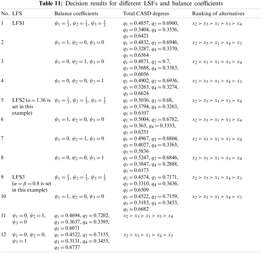
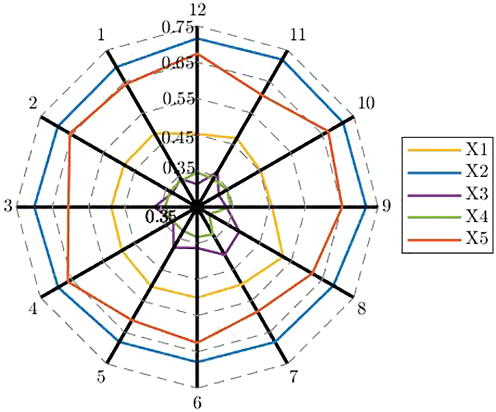
Figure 13: Demonstration of ranking results
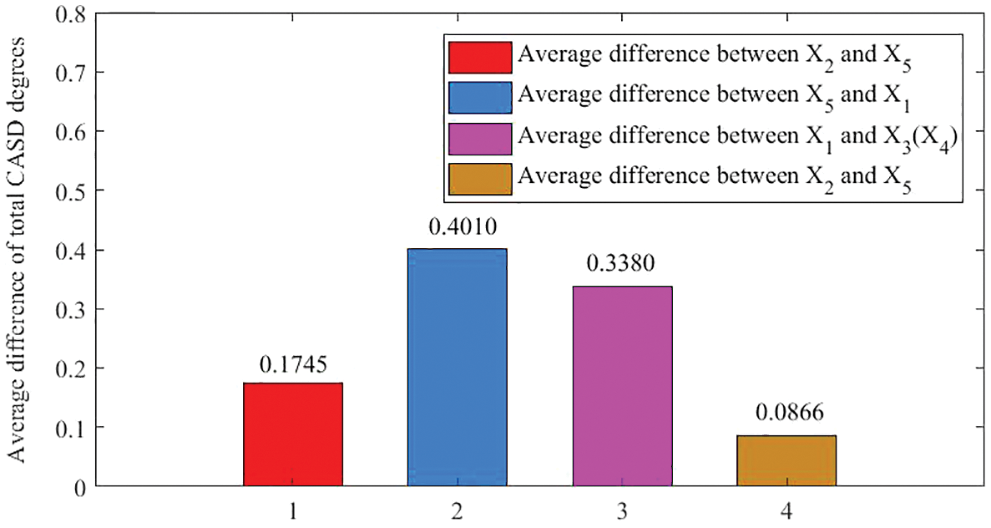
Figure 14: Average differences of total CASD degrees
As can be seen from Table 11 and Fig. 13, the ranking order of alternatives is
Furthermore, the proposed method can handle various decision situations and meet different DMs’ preferences by taking different LSFs and balance coefficients. Thus, the flexibility of the proposed method can be reflected by the acquired ranking results derived by various selections of LSFs and balance coefficients.
6 Comparison Analyses and Discussion
To justify the advantages of our proposal, comparison analyses with methods based on cloud and other classical MAGDM methods are conducted. Besides, a summary of transformation approaches with different evaluation forms is presented.
6.1 Comparison with Methods Based on Cloud
Peng et al. [23] proposed a new method based on cloud to handle MAGDM problems with PLTSs. Hu [32] proposed two methods based on comprehensive cloud aggregation operator to solve MAGDM problems with LHFSs. This paper proposes a novel method based on cloud for heterogeneous MAGDM, which could handle MAGDM problems with LT, PLTS, LHFS or one of them. Obviously, the aforesaid methods all are based on cloud. The proposed method could handle MAGDM problems in [23,32], while Peng et al.'s method [23] and Hu's methods [32] could not solve the problem of this paper. Thus, the proposed method has wider applicability. Except for wider applicability, other important distinguishing factors and superiorities of the proposed method are stated as follows:
(1) The cloud in [23] contains five characteristics, yet the values of left and right entropy are averaged into one in this paper, which greatly reduce the complexity of the following calculation. The transformation from LTs to clouds in [32] is based on the golden radio, while it is based on LSFs in this paper. The selection for LSFs and its related parameters makes the transformation more flexible and practical. In addition, this paper proposes regulation parameters for entropy and hyper entropy. DMs’ personalities can be reflected with the incorporation of regulation parameters in the transformation from LTs to clouds. Moreover, the modified ratios of LTs decrease the loss and distortion of evaluation information in the transformation from PLTSs (LHFSs) to C-PLTSs (C-LHFSs).
(2) The method in [23] determines the attribute weights only via maximizing deviation, while three perspectives are considered to obtain the attribute weights in this paper. Besides, the setting of balance coefficients enhances the flexibility of the proposed method. Moreover, three steps are needed to obtain attribute weights in [23], including determining the individual weights of criteria, determining the weights associated with groups (equivalent to DMs in this paper) and calculating the overall weights of attributes. By contrast, only one step is needed to obtain attribute weights by the proposed method, which reduces the complexity of the calculation greatly.
(3) The proposed approach to determining DMs’ weights is superior to [32]. Hu [32] and this paper both consider the number of LTs and corresponding indeterminacy degree in LHFS. However, if all the DMs only use one LT with different memberships in all LHFSs, the determination approach of DMs’ weights in [32] becomes invalid. For example,
It can be seen that
(4) The ranking of alternatives is based on the expected score values of clouds in [32]. The expected score values of clouds sometimes are unstable and may lead to inaccurate decision results. By contrast, the ranking of alternatives is based on the total CASD degree in this paper. Obviously, the ranking approach of this paper is more stable.
6.2 Comparison with Other Classical MAGDM Methods
Lin et al. [50] put forward two novel TOPSIS-ScoreC-PLTS and VIKOR-ScoreC-PLTS methods to handle MAGDM problems with PLTSs. This paper proposes a personalized comprehensive cloud-based method for heterogeneous MAGDM, which could handle MAGDM problems with LT, PLTS, LHFS or one of them. To justify the advantages of our proposal, comparison analyses with Lin et al.'s method [50] are conducted as follows:
(1) Solve the adapted example of this paper by the methods in [50]
Since Lin et al.'s method just cloud handle the MAGDM problems with PLTSs, we only retain the evaluations on
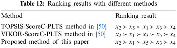
It is easy to find that
(2) Solve the example in [50] by the proposed method of this paper
The proposed method could handle MAGDM problems with LT, PLTS, LHFS or one of them. As a result, the proposed method could settle the example in [50] directly and the calculation results are as follows:
DM weight vector:
Attribute weight vector:
The total CASD degrees:
Therefore, the final ranking order is
The ranking order by method in [50] is
6.3 Comparison with Other Transformation Approaches
Previous studies [22–27,30–34] have proposed a lot of transformation approaches from LT and its’ extended forms to cloud and comprehensive clouds. A specific summary is shown in Table 13.
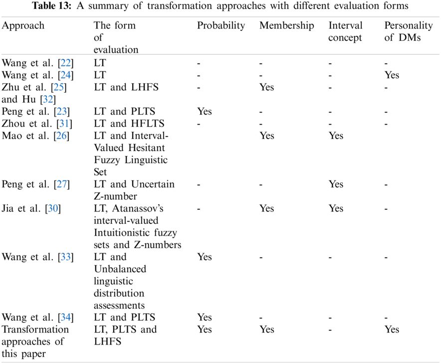
In summary, we find that most existing studies can only process LTs, or LTs with probability, or LTs with membership or LTs with interval concept. However, this paper provides the transformation approaches for LTs, LTs with probability and LTs with membership, simultaneously. Moreover, there are few studies that take DMs’ personalities into account during the transformation process. Although Wang et al. [24] introduced overlap parameter into the transformation process to reflect the DMs’ personality, the determination of overlap parameter is a little subjective. This paper proposes regulation parameters for entropy and hyper entropy and further incorporates them into the transformation process from LTs to clouds to reflect the different personalities of DMs. It is worth emphasizing that the determination of regulation parameters is totally objective. Apparently, the proposed transformation approaches of this paper are more applicable and effective.
This paper develops a personalized comprehensive cloud-based method for heterogeneous MAGDM, in which the evaluations of alternatives on attributes are represented as LTs, PLTSs and LHFSs. The validity of the proposed method is demonstrated with a site selection example of emergency medical waste disposal in COVID-19. The effectiveness, stability, flexibility and superiorities of the proposed method are proven by sensitivity and comparison analyses, respectively. Compared with the existing methods, the proposed method of this paper has the following prominent superiorities:
(1) With the proposed regulation parameters, the width and thickness of clouds for the corresponding LTS are different for different DMs, which makes the DMs’ personalities can be reflected in clouds. Besides, a novel approach to obtaining DM weight vector is constructed based on the proposed regulation parameters.
(2) The new transformation approaches from PLTS and LHFS to C-PLTS and C-LHFS decrease the loss and distortion of evaluation information.
(3) CASD relationship and CASD degree are initiated in this paper to compare clouds. With CASD relationship and CASD degree, alternatives in the form of clouds can be ranked and the ranking results are stable and effective. This innovation provides new perspective for pairwise comparisons of clouds.
(4) The comprehensive tri-objective programing constructed in this paper enables DMs to make a tradeoff among three different aspects. Multifaceted considerations enhance the stability of the proposed method and the setting of balance coefficients improves the flexibility of the proposed method.
Although an example of emergency medical waste disposal site selection in COVID-19 is illustrated to the effectiveness of the proposed method, and it is expected to be applied to more real-life decision-making problems, such as investment selection, supply chain management, and so on. More effective transformation approaches for other evaluation forms, especially LTs with interval concept are waiting for us to come up with and apply them to heterogeneous MAGDM problems. Additionally, how to extend some classical decision-making methods to heterogeneous MAGDM based on cloud is also very interesting and deserves to be studied in the future.
Funding Statement: This research was supported by the National Natural Science Foundation of China (Nos. 62141302, 11861034 and 71964014), the Humanities Social Science Programming Project of Ministry of Education of China (No. 20YJA630059), the Natural Science Foundation of Jiangxi Province of China (No. 20212BAB201011), and the Postgraduate Innovation Fund Project of Jiangxi Province (No. YC2020-S290).
Conflicts of Interest: The authors declare that they have no conflicts of interest to report regarding the present study.
1. Yu, S. M., Du, Z. J., Wang, J. Q., Luo, H. Y., Lin, X. D. (2021). Trust and behavior analysis-based fusion method for heterogeneous multiple attribute group decision-making. Computers & Industrial Engineering, 152(8), 106992. DOI 10.1016/j.cie.2020.106992. [Google Scholar] [CrossRef]
2. Boran, F. E., Genç, S., Kurt, M., Akay, D. (2009). A Multi-attributes intuitionistic fuzzy group decision making for supplier selection with TOPSIS method. Expert Systems with Applications, 36(8), 11363–11368. DOI 10.1016/j.eswa.2009.03.039. [Google Scholar] [CrossRef]
3. Liang, R. X., Wang, J. Q., Li, L. (2018). Multi-attributes group decision-making method based on interdependent inputs of single-valued trapezoidal neutrosophic information. Neural Computing & Applications, 30(1), 241–260. DOI 10.1007/s00521-016-2672-2. [Google Scholar] [CrossRef]
4. Qin, J. D., Liu, X. W., Pedrycz, W. (2017). An extended TODIM multi-attributes group decision making method for green supplier selection in interval type-2 fuzzy environment. European Journal of Operational Research, 258, 626–638. DOI 10.1016/j.ejor.2016.09.059. [Google Scholar] [CrossRef]
5. Wang, J. Q., Peng, J. J., Zhang, H. Y., Liu, T., Chen, X. H. (2015). An uncertain linguistic multi-attributes group decision-making method based on a cloud model. Group Decision and Negotiation, 24(1), 171–192. DOI 10.1007/s10726-014-9385-7. [Google Scholar] [CrossRef]
6. Tian, Z. P., Wang, J., Wang, J. Q., Zhang, H. Y. (2017). Simplified neutrosophic linguistic multi-attributes group decision-making approach to green product development. Group Decision and Negotiation, 26(3), 597–627. DOI 10.1007/s10726-016-9479-5. [Google Scholar] [CrossRef]
7. Pang, Q., Wang, H., Xu, Z. (2016). Probabilistic linguistic term sets in multi-attribute group decision making. Information Sciences, 369, 128–143. DOI 10.1016/j.ins.2016.06.021. [Google Scholar] [CrossRef]
8. Meng, F., Chen, X., Zhang, Q. (2014). Multi-attribute decision analysis under a linguistic hesitant fuzzy environment. Information Sciences, 267, 287–305. DOI 10.1016/j.ins.2014.02.012. [Google Scholar] [CrossRef]
9. Liu, A. H., Wan, S. P., Dong, J. Y. (2021). An axiomatic design-based mathematical programming method for heterogeneous multi-criteria group decision making with linguistic fuzzy truth degrees. Information Sciences, 571, 649–675. DOI 10.1016/j.ins.2021.04.091. [Google Scholar] [CrossRef]
10. Gao, Y., Li, D. S. (2019). A consensus model for heterogeneous multi-attribute group decision making with several attribute sets. Expert Systems with Applications, 125, 69–80. DOI 10.1016/j.eswa.2019.01.072. [Google Scholar] [CrossRef]
11. Wan, S. P., Zou, W. C., Dong, J. Y. (2020). Prospect theory based method for heterogeneous group decision making with hybrid truth degrees of alternative comparisons. Computers & Industrial Engineering, 141, 106285. DOI 10.1016/j.cie.2020.106285. [Google Scholar] [CrossRef]
12. Merigo, J. M., Palacios-Marques, D., Zeng, S. Z. (2016). Subjective and objective information in linguistic multi-criteria group decision making. European Journal of Operational Research, 248(2), 522–531. DOI 10.1016/j.ejor.2015.06.063. [Google Scholar] [CrossRef]
13. Merigo, J. M., Gil-Lafuente, A. M. (2013). Induced 2-tuple linguistic generalized aggregation operators and their application in decision-making. Information Sciences, 236, 1–16. DOI 10.1016/j.ins.2013.02.039. [Google Scholar] [CrossRef]
14. Li, D. Y., Liu, C., Gan, W. (2009). A new cognitive model: Cloud model. Wiley Subscription Services, 24(3), 357–375. DOI 10.1002/int.20340. [Google Scholar] [CrossRef]
15. Li, D. Y., Du, Y. (2007). Artificial intelligent with uncertainty. China: Journal of Software. [Google Scholar]
16. Zhang, H. Y., Ji, P., Wang, J. Q., Chen, X. H. (2016). A neutrosophic normal cloud and its application in decision making. Cognitive Computation, 8, 649–669. DOI 10.1007/s12559-016-9394-8. [Google Scholar] [CrossRef]
17. Li, D. Y. (1997). Knowledge representation in KDD based on linguistic atoms. Journal of Computer Science and Technology, 12(6), 481–496. DOI 10.1007/BF02947201. [Google Scholar] [CrossRef]
18. Li, D., Han, J., Shi, X., Man, C. (1998). Knowledge representation and discovery based on linguistic atoms. Knowledge-Based Systems, 10(7), 431–440. DOI 10.1016/S0950-7051(98)00038-0. [Google Scholar] [CrossRef]
19. Guan, X. J., Qian, L., Li, M. X., Zhou, L. G. (2017). Earthquake relief emergency logistics capacity evaluation model integrating cloud generalized information aggregation operators. Journal of Intelligent & Fuzzy Systems, 32(3), 2281–2294. DOI 10.3233/JIFS-16252. [Google Scholar] [CrossRef]
20. Deng, W. H., Wang, G. Y., Xu, J. (2016). Piecewise two-dimensional normal cloud representation for time-series data mining. Information Sciences, 374, 32–50. DOI 10.1016/j.ins.2016.09.027. [Google Scholar] [CrossRef]
21. Di, K. C., Li, D. Y., Li, D. R. (1999). Cloud theory and its applications in spatial data mining and knowledge discovery. Journal of Image and Graphics, 11(4), 930–935. DOI 10.3969/j.issn.1006-8961.1999.11.006. [Google Scholar] [CrossRef]
22. Wang, J. Q., Peng, L., Zhang, H. Y., Chen, X. H. (2014). Method of multi-attribute group decision-making based on cloud aggregation operators with linguistic information. Information Sciences, 274, 177–191. DOI 10.1016/j.ins.2014.02.130. [Google Scholar] [CrossRef]
23. Peng, H. G., Zhang, H. Y., Wang, J. Q. (2018). Cloud decision support model for selecting hotels on tripadvisor.com with probabilistic linguistic information. International Journal of Hospitality Management, 68, 124–138. DOI 10.1016/j.ijhm.2017.10.001. [Google Scholar] [CrossRef]
24. Wang, P., Xu, X., Cai, C., Huang, S. (2018). A linguistic large group decision making method based on the cloud model. IEEE Transactions on Fuzzy Systems, 26(6), 3314–3326. DOI 10.1109/TFUZZ.2018.2822242. [Google Scholar] [CrossRef]
25. Zhu, C. X., Zhu, L., Zhang, X. Z. (2016). Linguistic hesitant fuzzy power aggregation operators and their applications in multiple attribute decision-making. Information Sciences, 367, 809–826. DOI 10.1016/j.ins.2016.07.011. [Google Scholar] [CrossRef]
26. Mao, X. B., Hu, S. S., Dong, J. Y., Wan, S. P., Xu, G. L. (2018). Multi-attribute group decision making based on cloud aggregation operators under interval-valued hesitant fuzzy linguistic environment. International Journal of Fuzzy Systems, 20(7), 2273–2300. DOI 10.1007/s40815-018-0495-2. [Google Scholar] [CrossRef]
27. Peng, H. G., Zhang, H. Y., Wang, J. Q., Li, L. (2019). An uncertain z-number multicriteria group decision-making method with cloud models. Information Sciences, 501, 136–154. DOI 10.1016/j.ins.2019.05.090. [Google Scholar] [CrossRef]
28. Song, W., Zhu, J. (2019). A multistage risk decision making method for normal cloud model considering behavior characteristics. Applied Soft Computing Journal, 78, 393–406. DOI 10.1016/j.asoc.2019.02.033. [Google Scholar] [CrossRef]
29. Wang, P., Zhang, J., Zhang, W. W. (2021). Multi-granularity linguistic large group decision-making based on cloud model and multi-layer weight determination. Control and Decision, 36(9), 2257–2266. DOI 10.13195/j.kzyjc.2020.0102. [Google Scholar] [CrossRef]
30. Jia, Q., Hu, J., He, Q., Zhang, W., Safwat, E. (2021). A multicriteria group decision-making method based on AIVIFSs, z-numbers, and trapezium clouds. Information Sciences, 566, 38–56. DOI 10.1016/j.ins.2021.02.042. [Google Scholar] [CrossRef]
31. Zhou, J., Liu, L. F., Sun, L. J., Xiao, F. (2018). A Multi-criteria decision-making method for hesitant fuzzy linguistic term set based on the cloud model and evidence theory. Journal of Intelligent & Fuzzy Systems, 36(2), 1–12. DOI 10.3233/JIFS-18051. [Google Scholar] [CrossRef]
32. Hu, S. S. (2018). Multi-attribute group decision making based on comprehensive cloud under linguistic hesitant fuzzy environment and its application in ERP selection (Master Thesis). Jiangxi University of Finance and Economics, China. [Google Scholar]
33. Wang, X. K., Wang, Y. T., Zhang, H. Y., Wang, J. Q., Li, L. et al. (2021). An asymmetric trapezoidal cloud-based linguistic group decision-making method under unbalanced linguistic distribution assessments. Computers & Industrial Engineering, 160, 107457. DOI 10.1016/j.cie.2021.107457. [Google Scholar] [CrossRef]
34. Wang, X. K., Wang, S. H., Zhang, H. Y., Wang, J. Q., Li, L. (2021). The recommendation method for hotel selection under traveller preference characteristics: A cloud-based multi-criteria group decision support model. Group Decision and Negotiation, 30, 1433–1469. DOI 10.1007/s10726-021-09735-0. [Google Scholar] [CrossRef]
35. Xu, Z. S. (2005). Deviation measures of linguistic preference relations in group decision making. Omega, 33(3), 249–254. DOI 10.1016/j.omega.2004.04.008. [Google Scholar] [CrossRef]
36. Wang, J. Q., Peng, H. G., Zhang, H. Y., Wang, J. (2017). An extended outranking approach for multi-criteria decision-making problems with linguistic intuitionistic fuzzy numbers. Applied Soft Computing, 59, 462–474. DOI 10.1016/j.asoc.2017.06.013. [Google Scholar] [CrossRef]
37. Bao, G. Y., Lian, X. L., He, M., Wang, L. L. (2010). Improved two-tuple linguistic representation model based on new linguistic evaluation scale. Control and Decision, 25(5), 780–784. DOI 10.3724/SP.J.1087.2010.02828. [Google Scholar] [CrossRef]
38. Tversky, A., Kahneman, D. (1992). Advances in prospect theory: Cumulative representation of uncertainty. Journal of Risk and Uncertainty, 5(4), 297–323. DOI 10.1007/BF00122574. [Google Scholar] [CrossRef]
39. Li, D. Y., Meng, H. J., Shi, X. M. (1995). Membership clouds and membership cloud generator. Journal of Computer Research and Development, 32(6), 15–20. [Google Scholar]
40. Qin, K., Kai, X., Liu, F. L., Li, D. Y. (2011). Image segmentation based on histogram analysis utilizing the cloud model. Computers & Mathematics with Applications, 62(7), 2824–2833. DOI 10.1016/j.camwa.2011.07.048. [Google Scholar] [CrossRef]
41. Schmid, F., Trede, M. (1996). Testing for first-order stochastic dominance: A New distribution-free test. Journal of the Royal Statistical Society: Series D (The Statistician), 45(3), 371–380. [Google Scholar]
42. Chen, X., Liang, H. M., Gao, Y., Xu, W. J. (2020). A method based on the disappointment almost stochastic dominance degree for the multi-attribute decision making with linguistic distributions. Information Fusion, 54, 10–20. DOI 10.1016/j.inffus.2019.06.027. [Google Scholar] [CrossRef]
43. Wan, S. P., Li, D. F. (2013). Fuzzy LINMAP approach to heterogeneous MADM considering comparisons of alternatives with hesitation degrees. Omega, 41(6), 925–940. DOI 10.1016/j.omega.2012.12.002. [Google Scholar] [CrossRef]
44. Wang, H. L., Feng, Y. Q. (2005). On multiple attribute group decision making with linguistic assessment information based on cloud model. Control and Decision, 20(6), 679–685. DOI 10.13195/j.cd.2005.06.79.wanghl.017. [Google Scholar] [CrossRef]
45. Wang, Y., Tian, L., Wu, Z. (2021). Trust modeling based on probabilistic linguistic term sets and the MULTIMOORA method. Expert Systems with Applications, 165(4), 113817. DOI 10.1016/j.eswa.2020.113817. [Google Scholar] [CrossRef]
46. Zhao, K., Gao, J. W., Qi, Z. Q., Li, C. B. (2015). Multi-criteria risky decision-making approach based on prospect theory and cloud model. Control and Decision, 30(3), 395–402. DOI 10.13195/j.kzyjc.2013.1773. [Google Scholar] [CrossRef]
47. Wang, Y. (1997). Using the method of maximizing deviation to make decision for multi-indices. Journal of Systems Engineering and Electronics, 8(3), 21–26. [Google Scholar]
48. Liu, X. D., Zhu, J. J., Zhang, S. T., Liu, G. D. (2016). Hesitant fuzzy multiple attribute decision making method based on optimization of attribute weights. Control and Decision, 31(2), 297–302. DOI 10.13195/j.kzyjc.2014.1931. [Google Scholar] [CrossRef]
49. Xu, Z. S., Xia, M. M. (2012). Hesitant fuzzy entropy and cross-entropy and their use in multi-attribute decision-making. International Journal of Intelligent Systems, 27(9), 799–822. DOI 10.1002/int.21548. [Google Scholar] [CrossRef]
50. Lin, M. W., Chen, Z. Y., Xu, Z. S., Gou, X. J., Herrera, F. (2021). Score function based on concentration degree for probabilistic linguistic term sets: an application to TOPSIS and VIKOR. Information Sciences, 551, 270–290. DOI 10.1016/j.ins.2020.10.061. [Google Scholar] [CrossRef]
 | This work is licensed under a Creative Commons Attribution 4.0 International License, which permits unrestricted use, distribution, and reproduction in any medium, provided the original work is properly cited. |