| Computer Modeling in Engineering & Sciences |
DOI: 10.32604/cmes.2022.019160
ARTICLE
Weakly Singular Symmetric Galerkin Boundary Element Method for Fracture Analysis of Three-Dimensional Structures Considering Rotational Inertia and Gravitational Forces
1School of Aeronautic Science and Engineering, Beihang University, Beijing, China
2Department of Mechanical Engineering, Texas Tech University, Lubbock, USA
*Corresponding Authors: Xuan Zhou. Email: zhoux@buaa.edu.cn; Leiting Dong. Email: ltdong@buaa.edu.cn
Received: 06 September 2021; Accepted: 26 November 2021
Abstract: The Symmetric Galerkin Boundary Element Method is advantageous for the linear elastic fracture and crack-growth analysis of solid structures, because only boundary and crack-surface elements are needed. However, for engineering structures subjected to body forces such as rotational inertia and gravitational loads, additional domain integral terms in the Galerkin boundary integral equation will necessitate meshing of the interior of the domain. In this study, weakly-singular SGBEM for fracture analysis of three-dimensional structures considering rotational inertia and gravitational forces are developed. By using divergence theorem or alternatively the radial integration method, the domain integral terms caused by body forces are transformed into boundary integrals. And due to the weak singularity of the formulated boundary integral equations, a simple Gauss-Legendre quadrature with a few integral points is sufficient for numerically evaluating the SGBEM equations. Some numerical examples are presented to verify this approach and results are compared with benchmark solutions.
Keywords: Symmetric Galerkin boundary element method; rotational inertia; gravitational force; weak singularity; stress intensity factor
Nomenclature
| Young’s modulus | |
| Poisson’s ratio | |
| Shear modulus | |
| Density | |
| Gravitational acceleration | |
| Angular velocity |
The Symmetric Galerkin Boundary Element Method (SGBEM) [1–3] has gained increasing popularity in fracture and crack-growth analysis of solid structures due to its attractive features of symmetric coefficient matrices, weak-singularity, and that only boundary & crack-surface elements are needed. The papers by Bonnet et al. [3–5] are devoted to the formulation, numerical evaluation and implementation of SGBEM. Atluri et al. [6–9] utilized a simple and straightforward methodology to develop regularized traction Boundary Integral Equations (tBIE) for two and three-dimensional linear-elastic solids containing cracks, and also developed weakly-singular SGBEMs for the fracture and fatigue analysis of various complex structures. However, for the fracture mechanics problems such as turbine discs and turbine blades of aircraft engines, concrete gravity dam, etc., SGBEM may lose its advantages, because evaluation of domain integral terms resulting from body forces such as rotational inertia and gravitational loads leads to the meshing of the interior of the domain. For this reason, a method to evaluate such domain integral terms using only boundary meshes, is desired to efficiently analyze cracked structures considering body forces with SGBEM.
For the conventional collocation boundary element method based on Somigliana’s identity for the displacement vector, a few methods were developed for this purpose. Considering centrifugal loads presented in rotating gas turbines, Cruse et al. [10,11] transformed domain integrals to boundary integrals by utilizing the divergence theorem. By making use of the Galerkin vector or the Green’s second identity, Danson [12] transformed the volume integral terms to boundary integral terms, for three kinds of body forces, i.e., gravitational loads, the rotational inertia and steady-state thermal loads. Gao [13] also developed a radial integration technique and applied it to deal with various body forces. Brebbia et al. [14] developed the dual reciprocity method [15] which converts the associated domain integrals into boundary integrals by using a series of basis functions to approximate the body force fields. Brebbia et al. [16] extended the idea of dual reciprocity and proposed another approach, multiple reciprocity method.
Different from the conventional collocation boundary element method [17–19] based on the Somigliana’s identity, formulations of SGBEM [5,8,20] result in weak-form displacement Boundary Integral Equations (dBIE) and weak-form traction Boundary Integral Equations (tBIE). As a matter of fact, the domain integrals caused by body forces appear both in dBIE and tBIE. Moreover, it is beneficial to use tBIE to derive weak-form equations on crack-surfaces, where displacement discontinuities are to be solved as unknowns [5]. Thus, if SGBEM is utilized for linear fracture analysis of cracked structures, while for domain integrals appearing in dBIE, one may refer to the above-mentioned transformation techniques, the treatment for domain integral terms appearing in tBIE needs further study.
This paper presents the weakly singular traction boundary integral equation for solids undergoing rotational inertia and gravitational Loads. By using the divergence theorem (div) or the radial integration method (RIM), domain integrals induced by rotational inertia or gravitational forces are transformed into boundary integrals correspondingly. The derived formulas show that these transformed boundary integral terms have no influence upon the coefficient matrix of SGBEM, but only affect the right-hand-side vector. The transformed boundary integral terms derived by the divergence theorem and radial integration method, possessing
This paper is organized as follows. In Section 2, transformation from domain integrals induced by gravitational and rotational inertia forces to the boundary integrals by div or RIM respectively is carried out. Some numerical examples for solids undergoing rotational inertia or gravitational loads are presented in Sections 3 and 4 with and without cracks correspondingly. In Section 5, we complete this paper with some concluding remarks.
2 Weakly Singular Galerkin Boundary Integral Equations and Boundary Element Method with Rota- tional Inertia and Gravitational Loads
Consider a linear elastic, homogenous and isotropic solid undergoing an infinitesimal elasto-static deformation, as shown in Fig. 1.

Figure 1: A solution domain with source point
The symmetric Galerkin formulations of displacement and traction Boundary Integral Equations (d & tBIE) for linear elastic solids can be found in [8]. The derivation of the conventional boundary element method and SGBEM [5,8,20] generally ignored body forces. Here, the domain integrals considering body forces are added in the equations:
In the above two equations, if the domain integral or boundary integral is with respect to the field point, the integral domain is denoted by
where
In this paper, the domain integral:
appearing in traction boundary integral Eq. (2) considering rotational inertia and gravitational loads is transformed into weakly singular boundary integral, using the divergence theorem or the radial integration method.
The radial integration method is introduced here briefly. For further details, one may refer to [13]. Domain integral on the left-hand-side of Eq. (5) with a general function

Figure 2: Cartesian and spherical coordinate systems
In the spherical coordinate system
where
In the spherical coordinate system, the area of infinitesimal element
If the field point is on the boundary
where

Figure 3: Spherical surface
By some derivations, the domain integral can be rewritten as
where
where
Some useful formulas related to
In Subsections 2.1 and 2.2, the domain integral terms with rotational inertia and gravitational loads in tBIE are transformed into weakly singular boundary integral terms by two methods of divergence theorem and radial integration method, respectively.
2.1 Transformation of Domain Integrals with Gravitational Loads to Boundary Integrals
Consider a solid body with a constant mass density
In this section, the body force
where
Thus, the constant gravity force
2.1.1 Using Divergence Theorem to Transform Domain Integrals with Gravitational Forces
Substitution of Eq. (19) into Eq. (26), we have
Substituting Eq. (22) into Eq. (27), we have
Using divergence theorem and Eq. (16), we can get that
Note that, a singularity of
2.1.2 Using the Radial Integration Method to Transform Domain Integrals with Gravitational Forces
Using radial integration method, Eq. (26) can be rewritten as
where
From Eq. (13) and Fig. 2, one can find that
Note that, when the field point approaches the source point,
2.2 Transform Domain Integrals with Rotational Inertia to Boundary Integrals
About an analytical expression of the rotational inertial force in detail, one may refer to [19]. Here we introduce it briefly. Consider a solid body of uniform mass density

Figure 4: The rotational axis passing through the origin of Cartesian coordinate system
By the D’Alembert’s principle, body force resulting from the rotational inertia is
Eq. (33) may be written in index notation as
where
Note that
Then this dynamic problem can be treated as an elastostatics problem. Using Eqs. (4), (25) and (34), we get
2.2.1 Using Divergence Theorem to Transform Domain Integrals with Inertial Force
Similar to the derivation of Eq. (28), the inertial force domain integrals with the rotational inertia can be written as
Substituting Eqs. (39) and (40) into Eq. (38) and using Eq. (17),
We get
Then using the divergence theorem, we get
Note that the boundary integrals in Eq. (42) have the property of
2.2.2 Using Radial Integration method to Transform Domain Integrals with Inertial Force
Using radial integration method, Eq. (37) may be rewritten as
As is mentioned above,
Note that, for radial integral
Eq. (46) is the boundary integral form with the rotational inertia force obtained by the radial integration method.
2.3 Weakly-Singular SGBEM with Numerical Implementation
We have obtained weakly singular boundary integrals transformed from domain integrals considering rotational inertia and gravitational loads by the divergence theorem or radial integration method. In this section, the displacement and traction boundary integral equations considering crack surfaces and rotational inertia and gravitational loads are given. Then numerical evaluation of weakly singular double layer surface integrals by using quadrilateral elements is introduced briefly.
2.3.1 Traction and Displacement BIEs Considering Rotational Inertia and Gravitational Loads by Divergence Theorem
Consider a crack embedded in the domain
where
where

Figure 5: Displacement discontinuity in domain
If the weak-form traction boundary integral equation is applied on
And if the weak-form traction boundary integral equation is applied on the crack surfaces
Finally, the weak-form displacement boundary integral equation is applied on the prescribed displacement boundary surfaces
Eqs. (49)–(51) are the weakly-singular traction and displacement boundary integral equations considering rotational inertia and gravitational loads obtained by using divergence theorem.
2.3.2 Traction and Displacement BIEs Considering Rotational Inertia and Gravitational Loads by the Radial Integration Method
Similar to Eqs. (49)–(51), the weakly-singular traction and displace BIE considering rotational inertia and gravitational loads by radial integration method can be written as follows:
By the same discretization procedure mentioned above for Eqs. (52)–(54), the SGBEM equations obtained by radial integration method can be obtained, and we denote this as SGBEM-RIM in this paper.
It can be seen that, for Eqs. (49), (50) using the divergence theorem, there exists
2.3.3 Numerical Evaluation of Weakly-Singular Double Surface Integrals Using Quadrilateral Elements
In this paper, 8-noded quadrilateral isoparametric elements are selected for the numerical implementation, and quarter-point singular quadrilateral elements with two mid-side nodes shifted towards the crack front as shown in Fig. 6 are adopted at the crack front. For the numerical evaluation of double surface integrals by quadrilateral isoparametric elements in detail, one may refer to [3], here it is introduced briefly.

Figure 6: A quarter-point singular quadrilateral element
As shown in Fig. 7, there are four quadrilateral elements A, B, C, D. In the computation of the double layer surface (

Figure 7: Cases of pairs of quadrilateral elements
For a pair of distinct elements, standard isoparametric coordinate transformation is used together with the standard Gauss-Legendre quadrature. As an example, the double layer surface integral considering gravitational loads obtained by the divergence theorem in Eq. (49) is considered at here.
For simplicity, we rewrite it as
where
For cases of coincident elements, adjacent elements sharing one edge, adjacent elements sharing one vertex, further coordinate transformations are given in below to cancel the singularity caused by
For a pair of coincident elements, local isoparametric coordinates are shown in Fig. 8. The boundary integral domain is partitioned into 8 subdomains. For each case we may implement a further transformation of variables listed in Table 1.

Figure 8: Isoparametric coordinates for a pair of coincident elements

In Table 1,
The Jacobian for such a variable transformation can be used to cancel the singularity in Eq. (56):
For a pair of coincident elements, Eq. (56) can be rewritten as
For a pair of common-edge elements, local isoparametric coordinates are shown in Fig. 9.

Figure 9: Local isoparametric coordinates for a pair of common-edge elements
This boundary integral domain is partitioned into 6 subdomains. For each case we may implement a transformation of variables listed in Table 2.

In Table 2,
Jacobians of the variable transformation are
For a pair of elements with a common vertex, local isoparametric coordinates is shown in Fig. 10.

Figure 10: Isoparametric coordinates for a pair of elements with a common vertex
This boundary integral domain is partitioned into 4 subdomains. For each case, a transformation of variables listed in Table 3 is implemented.

Variables
The Jacobian of the variable transformation can be used to cancel the singularity in Eq. (56):
3 Numerical Examples without Cracks
In this section and the next section some examples without or with crack are implemented respectively to verify SGBEM-div or SGBEM-RIM developed in Section 2.
3.1 Numerical Test of the Effect of the Number of Integration Points
In this section, the double surface integral term in Eq. (55), for a pair of coincident square elements, is evaluated using the quadrature method given in Section 2.3.3, considering the problem of a cube of two kinds of meshes undergoing gravity given in Section 3.2. Fig. 11 shows the logarithmic value of the absolute value of relative errors for the numerical integration of both a pair of square elements and a pair of distorted elements. The error is very small when the number of Gauss integration points is larger than 6. Thus, 8 gauss points are used for the evaluation of double layer surface integrals in the following examples except for the cube undergoing gravitational loads in Section 3.2.
The effect of the number of integration points is shown in Fig. 12, where the relative error is defined as follows:

Figure 11: Relative errors for the evaluated weakly-singular boundary integral
3.2 A Cube Undergoing Gravitational Loads
We consider a cube with dimensions of
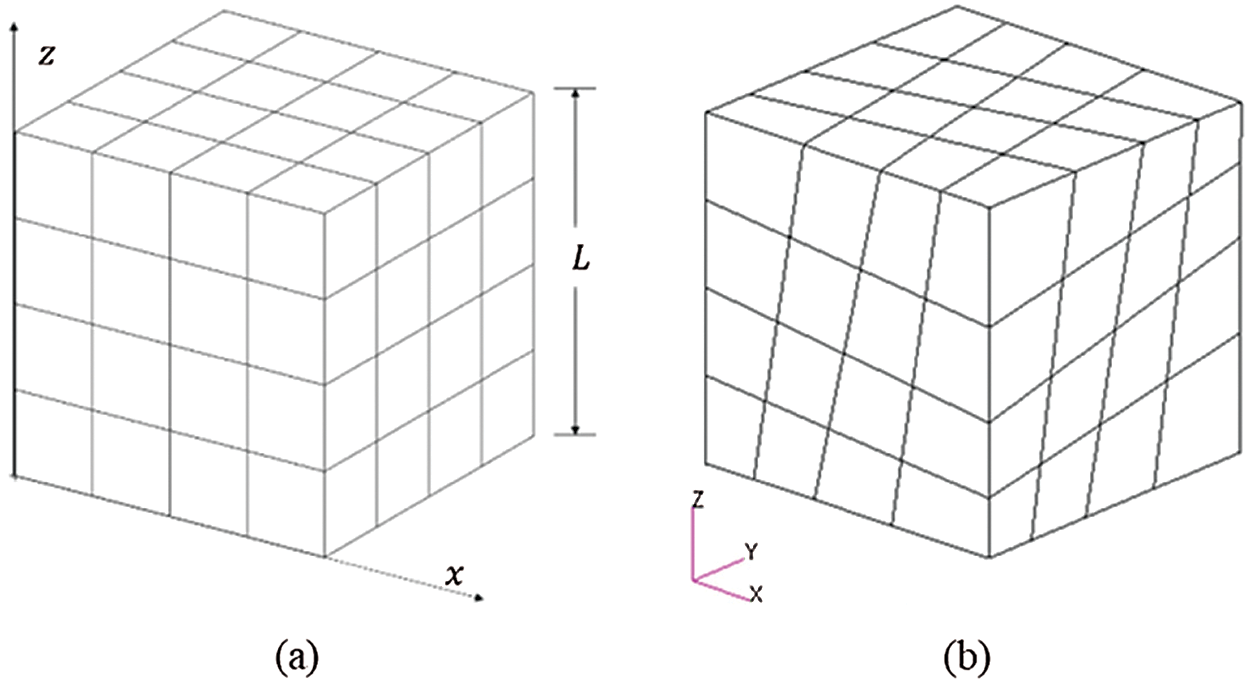
Figure 12: Mesh of a cube (a) elements being square, (b) elements being distorted
The gravitational force
Because the analytical solution is only quadratic with respect to z coordinate, 3 Gauss points are used for the evaluation of vertical displacements along the direction

In the second example, a disk with inner radius of 0.1m and outer radius of 0.2 m, rotating at a constant angular speed
can be found in [23] where

Figure 13: A rotating disk

Figure 14: SGBEM dense mesh of the rotating disk
Table 5 shows the computed radial displacements with the mesh shown in Fig. 14. “Exact” denotes exact solutions by the Eq. (61). For each point, “Maximum error” of SGBEM-div and SGBEM-RIM is computed with the exact solution as the reference. As can be seen, computational results by SGBEM-div and SGBEM-RIM are in excellent agreement with the exact solutions.

4 Numerical Examples with Cracks
In this section, numerical examples with cracked solids considering body forces are given. In each example, after obtaining the displacement discontinuities for the quarter-point node using the developed SGBEM method, displacement extrapolation is used to calculate the stress intensity factors.
4.1 A Cuboid Hanging under Its Own Weight with a Through-Thickness Crack
Consider a solid cuboid with a crack of length 2a (see Fig. 15) under gravitational loads [24], where l = 4, b = 1, h = 0.5l, a = 0.1, t = 0.2, ρg = −10. The elastic constants are chosen to be E = 1000 and ν = 0.

Figure 15: A cracked cuboid hanging under its own weight
Computed stress intensity factors are presented in Table 6, in which “Error” means the relative error between SGBEM--div and FEM solution. For this through-thickness crack,

4.2 A Rotating Disk with a through-Thickness Crack
A rotating disk with a through-thickness crack (a = 0.03 m) is computed shown in Fig. 16. The rotating disk is identical to the disk in Section 3.3. Again, excellent agreement between the computed SGBEM results and FEM results are shown in Tables 7 and 8.

Figure 16: SGBEM mesh of a cracked rotating disk


4.3 A Rotating Disk with Semi-Elliptic Surface Cracks
This section gives a series of results for a cracked disk in Fig. 17 with various semi-elliptic surface cracks, shown in Fig. 18. All the parameters of this disk are identical to that of disk in Section 3, except for the semi-elliptic cracks. Various semi-elliptic cracks with a fixed depth (a = 0.004 m), and various semi-elliptic cracks with a fixed length/depth ratio (b/a = 2), are computed using both SGBEM-div and SGBEM-RIM.

Figure 17: A disk with a semi-elliptic surface crack

Figure 18: Various semi-elliptic cracks with a fixed depth (a = 0.004 m), and various semi-elliptic cracks with a fixed length/depth ratio (b/a = 2)
For simplicity, we give the stress intensity factor KI at point P, i.e., the deepest point of various semi-elliptic cracks, as shown in Figs. 19, and 20. These results can be used for the benchmark solutions for future studies.

Figure 19: KI at the deepest point of semi-elliptic cracks with a fixed depth (a = 0.004 m)

Figure 20: KI at the deepest point of semi-elliptic cracks with a fixed length/depth ratio (b/a = 2)
In this paper, weakly-singular SGBEM for fracture analysis of three-dimensional structures considering rotational inertia and gravitational forces is developed. By using the divergence theorem (div) or the radial integration method (RIM), rotational inertia or gravitational forces induced domain integrals are transformed into boundary integrals. The derived boundary integral terms with the gravitational and inertial forces are weakly-singular, which only influence the SGBEM right-hand-side vector.
Several numerical examples of solids with and without cracks undergoing body forces are studied. The calculated stress intensity factors and displacements show high accuracy compared with reference solutions. The test of numerical integration also shows that only a small number of quadrature points are needed.
The symmetric Galerkin boundary element method considering gravity and inertia loads presented in this paper appears promising in the fracture analysis of structural components with body forces, such as dams and rotating machineries. Furthermore, with some effort, the methodology given in this study can also be extended to deal with domain integrals for SGBEM with thermoelastic problems, which will be given in a subsequent work.
Funding Statement: The first four authors acknowledge the support of the National Natural Science Foundation of China (12072011).
Conflicts of Interest: The authors declare that they have no conflicts of interest to report regarding the present study.
1. Sutradhar, A., Paulino, G. H., Gray, L. J. (2008). Symmetric galerkin boundary element method. Berlin, Heidelberg: Springer. [Google Scholar]
2. Bonnet, M., Maier, G., Polizzotto, C. (1998). Symmetric galerkin boundary element methods. Applied Mechanics Reviews, 51(11), 669–704. DOI 10.1115/1.3098983. [Google Scholar] [CrossRef]
3. Novati, G., Frangi, A. (2002). Symmetric galerkin BEM in 3D elasticity: Computational aspects and applications to fracture mechanics. In: Selected topics in boundary integral formulations for solids and fluids. Vienna: Springer. [Google Scholar]
4. Bonnet, M. (1999). Boundary integral equation methods for solids and fluids. Meccanica, 34(4), 301–302. DOI 10.1023/A:1004795120236. [Google Scholar] [CrossRef]
5. Li, S., Mear, M. E. (1998). Singularity-reduced integral equations for displacement discontinuities in three-dimensional linear elastic media. International Journal of Fracture, 93(1), 87–114. DOI 10.1023/A:1007513307368. [Google Scholar] [CrossRef]
6. Okada, H., Rajiyah, H., Atluri, S. N. (1988). A novel displacement gradient boundary element method for elastic stress analysis with high accuracy. Journal of Applied Mechanics, 55(4), 786–794. DOI 10.1115/1.3173723. [Google Scholar] [CrossRef]
7. Okada, H., Rajiyah, H., Atluri, S. N. (1989). Non-hyper-singular integral-representations for velocity (displacement) gradients in elastic/plastic solids (small or finite deformations). Computational Mechanics, 4(3), 165–175. DOI 10.1007/BF00296664. [Google Scholar] [CrossRef]
8. Han, Z. D., Atluri, S. N. (2003). On simple formulations of weakly-singular traction & displacement BIE, and their solutions through Petrov-Galerkin approaches. Computer Modeling in Engineering & Sciences, 4(1), 5–20. DOI 10.1.1.610.8720. [Google Scholar]
9. Dong, L. T., Atluri, S. N. (2012). SGBEM (Using non-hyper-singular traction BIEand super elements, for non-collinear fatigue-growth analyses of cracks in stiffened panels with composite-patch repairs. Computer Modeling in Engineering & Sciences, 89(5), 417–458. DOI 10.3970/cmes.2012.089.417. [Google Scholar] [CrossRef]
10. Cruse, T. A. (1975). Boundary-integral equation method for three-dimensional elastic fracture mechanics analysis. AFOSR-TR-75-0813 Interim Report. [Google Scholar]
11. Cruse, T. A., Snow, D. W., Wilson, R. B. (1977). Numerical solutions in axisymmetric elasticity. Computers & Structures, 7(3), 445–451. DOI 10.1016/0045-7949(77)90081-5. [Google Scholar] [CrossRef]
12. Danson, D. J. (1981). A boundary element formulation of problems in linear isotropic elasticity with body forces. In: Boundary element methods. Berlin, Heidelberg: Springer. [Google Scholar]
13. Gao, X. W. (2002). The radial integration method for evaluation of domain integrals with boundary-only discretization. Engineering Analysis with Boundary Elements, 26(10), 905–916. DOI 10.1016/S0955-7997(02)00039-5. [Google Scholar] [CrossRef]
14. Nardini, D., Brebbia, C. A. (1983). A new approach to free vibration analysis using boundary elements. Applied Mathematical Modelling, 7(3), 157–162. DOI 10.1016/0307-904X(83)90003-3. [Google Scholar] [CrossRef]
15. Partridge, P. W., Brebbia, C. A., Wrobel, L. C. (1992). The dual reciprocity boundary element method. Southampton Boston: Computational Mechanics Publications. [Google Scholar]
16. Nowak, A. J., Brebbia, C. A. (1989). The multiple-reciprocity method. A new approach for transforming BEM domain integrals to the boundary. Engineering Analysis with Boundary Elements, 6(3), 164–167. DOI 10.1016/0955-7997(89)90032-5. [Google Scholar] [CrossRef]
17. Aliabadi, F. M. H. (2018). Boundary element methods. In: Encyclopedia of continuum mechanics. Berlin, Heidelberg: Springer. [Google Scholar]
18. Brebbia, C. A. (2017). The birth of the boundary element method from conception to application. Engineering Analysis with Boundary Elements, 77(4), iii–x. DOI 10.1016/j.enganabound.2016.12.001. [Google Scholar] [CrossRef]
19. Brebbia, C. A. (1983). Progress in boundary element methods, vol. 2. New York: Springer. [Google Scholar]
20. Frangi, A., Novati, G., Springhetti, R., Rovizzi, M. (2002). 3D fracture analysis by the symmetric Galerkin BEM. Computational Mechanics, 28(3–4), 220–232. DOI 10.1007/s00466-001-0283-x. [Google Scholar] [CrossRef]
21. Fung, Y., Tong, P., Chen, X. (2017). Classical and computational solid mechanics. New Jersey: World Scientific. [Google Scholar]
22. de Klerk, J. H. (2011). Building a body of knowledge: Cauchy principal value and hypersingular integrals. AIP Conference Proceedings, 1389(1), 456–459. DOI 10.1063/1.3636762. [Google Scholar] [CrossRef]
23. Timoshenko, S. P., Goodier, J. N. (1970). Theory of elasticity. New York: McGraw-Hill. [Google Scholar]
24. Ostanin, I. A., Mogilevskaya, S. G., Labuz, J. F., Napier, J. (2011). Complex variables boundary element method for elasticity problems with constant body force. Engineering Analysis with Boundary Elements, 35(4), 623–630. DOI 10.1016/j.enganabound.2010.11.008. [Google Scholar] [CrossRef]
Kernel functions listed here are utilized in the numerical implementation of the SGBEM. Kernel functions (A1)–(A3) appear in the displacement boundary integral equation; kernel functions (A2)–(A4) appear in the traction boundary integral equation.
 | This work is licensed under a Creative Commons Attribution 4.0 International License, which permits unrestricted use, distribution, and reproduction in any medium, provided the original work is properly cited. |