Computer Modeling in Engineering & Sciences

DOI: 10.32604/cmes.2022.019991

ARTICLE

Discrete Element Simulations of Ice Load and Mooring Force on Moored Structure in Level Ice

Hongri Zhu and Shunying Ji*

State Key Laboratory of Structural Analysis for Industrial Equipment, Dalian University of Technology, Dalian, 116024, China
*Corresponding Author: Shunying Ji. Email: jisy@dlut.edu.cn
Received: 28 October 2021; Accepted: 04 January 2022

1  Introduction

Floating structures are prospective engineering equipment used for oil exploration and exploitation in the Arctic and sub-Arctic regions. They are cost-effective in deep waters and maneuverable in harsh environments. The mooring system is still the preferred choice for the station-keeping of floating structures, particularly under heavy ice conditions, although many researchers are exploring the feasibility of dynamic positions in ice-infested sea. Among the various types of ice features in the Arctic, level ice is the most common challenge for station-keeping capacity of floating structures and controls the design load levels in many cases. Therefore, it is necessary to develop an effective numerical method for predicting the ice load and mooring system response of moored structures in level ice.

As the most direct research method, a monitoring project on the ice load has been conducted for more than 10 years on the floating offshore structure, Kulluk, in the Beaufort Sea. The overall trending of the ice load under different ice conditions was determined based on the field measurements [1]. Further research on the ice load on moored structures was conducted based on model tests. Løset et al. [2] evaluated the feasibility of the mooring system of a submerged turret loading concept in level ice, broken ice and pressure ridges through model tests. Ettema et al. [3] and Dalane [4] researched the effect of mooring stiffness and pitch motion, respectively, on the ice load of moored conical platforms using basin model tests. Karulin et al. [5] analyzed characteristics of ice interaction with multi-legged structures based on a semi-submersible platform model. Although the results from those model test campaigns are valuable for studying the ice load of moored structures, their application is limited by the complexity of ice properties and scaling effects.

Numerical methods, especially the meshfree methods, are suitable to simulate the whole process of the ice-structure interaction at a full scale. Song et al. [6–8] proposed a state-based peridynamic model and a bond-based peridynamic de-icing model to simulate the quasi-brittle failure and coupled thermo-mechanical behavior of ice, respectively. Based on the ice failure model and the ice resistance formula [8,9], Nguyen et al. [10] and Zhou et al. [11] simulated the station-keeping performance of moored vessels with different control strategies in level ice. Further, Zhou et al. [12] considered the broken ice transport underwater and the corresponding ice accumulation force on moored ship according to the ISO (19906) code. The accuracy of the semi-analytic methods depends on the experimental data and related assumptions. The DEM method has been extensively applied to simulatie ice-structure interactions and initially focused on modeling broken ice [13–15]. Ji et al. [16,17] developed a bonded spherical discrete element method using the GPU parallel technology to simulate the fracture and movement of level ice. They also studied quantitatively the relationship between DEM computational parameters and macroscopic mechanical properties of sea ice through the numerical simulations of the uniaxial compression and three-point bending tests.

Previous numerical studies on moored structures in icy regions focused on ice actions, and the mooring system was often simplified as a linear or nonlinear spring [18,19]. However, the spring model neglects the dynamic response and hydrodynamic loads of mooring lines, which is critical to mooring system stability [20]. The lumped mass method [21] and nonlinear finite element method (FEM) [22] are the main methods used for the dynamic simulation of mooring lines in time domain. Recently, many researchers adopted the DEM method to model flexible structures because of its advantages in simulating the large deformation and complex contact. Jia [23] calculated the bending, torsion and winding of the cable, and analyzed the influence of different winding methods on the overall mechanical properties of the cable bundles based on DEM. Zhu et al. [24] constructed barriers using spherical elements with Timoshenko beam bonding model and simulated the interaction between rock flows and barriers. Those studies demonstrate the DEM is suitable for modeling mooring lines subjected to the action of complex environmental factors such as ice, waves and sea beds.

In this study, we applied the spherical discrete element method with the parallel bond model to construct the level ice and mooring lines of floating structures. We validated the accuracy of the mooring line by comparing the DEM numerical results with the nonlinear FEM solutions and experimental results. The effects of ice thickness on the ice load and dynamic response of a semi-submersible structure was studied based on the DEM results.

2  The Discrete Element Method for Level Ice and Mooring System

The DEM models of level ice and mooring lines are based on spherical discrete elements with the parallel bond model. The different mechanical properties of the two structures are defined with different element configurations and computational parameters.

2.1 Parallel Bond Model of Spherical Discrete Elements

In the parallel bond model, two adjacent elements are bonded by a virtual disk lying on the contact plane and centered at the contact point, as shown in Fig. 1 [25]. The bonding disk can transmit elastic force and moment to prevent the relative motion between the two bonded elements. The bonding force and moment can be resolved into normal and shear components associated with the contact plane and denoted by Fn,Fs,Mt and Mb. The increments of the components are calculated as Eqs. (1) and (2):

ΔFn=k¯nAΔUn;ΔFs=−k¯sAΔUs(1)

ΔMt=−k¯sJΔθn;ΔMb=−k¯nIΔθs(2)

where k¯n and k¯s are the normal stiffness and shear stiffness on unit area of the bonding disk respectively. ΔUn and Δθn are the relative normal and shear displacement (rotation) increments at the two ends of the bond, and ΔUs and Δθs are the corresponding shear displacement (rotation) increments. The bonding disk has a radius R¯; the section area, moment of inertia, and polar moment of inertia of the disk are calculated as A=πR2, I=14πR4, J=12πR4, respectively.

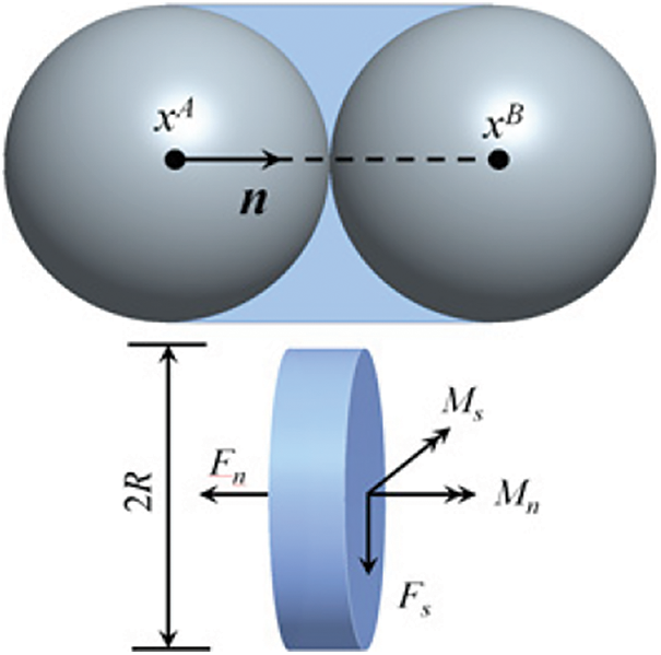
Figure 1: Parallel bond model in the DEM method

2.2 The Discrete Element Method of Level Ice

The level ice model was established by the bonded spherical elements arranged in Hexagonal Closest Packed (HCP) type, as shown in Fig. 2. The brittle fracture behavior of level ice can be modeled through breakage of the parallel bonds between elements. Bond failure occurs when the maximum normal or shear stresses on the contact plane exceed the corresponding strength. The stresses distribution on the bonding disk is defined based on the beam assumption, the max normal stress σmax and the shear stress τmax can be calculated as Eqs. (3) and (4) [25]:

σmax=−FnA+|Mb|IR¯(3)

τmax=|Fs|A+|Mt|JR¯(4)

The shear strength follows the Mohr-Coulomb criterion and is in proportion to the maximum normal stresses σmax. The shear strength equation can be written as follows:

τc=μσmax+σbs(5)

In Eq. (5), μ is the inner friction coefficient, and σbs is the shear cohesive strength.

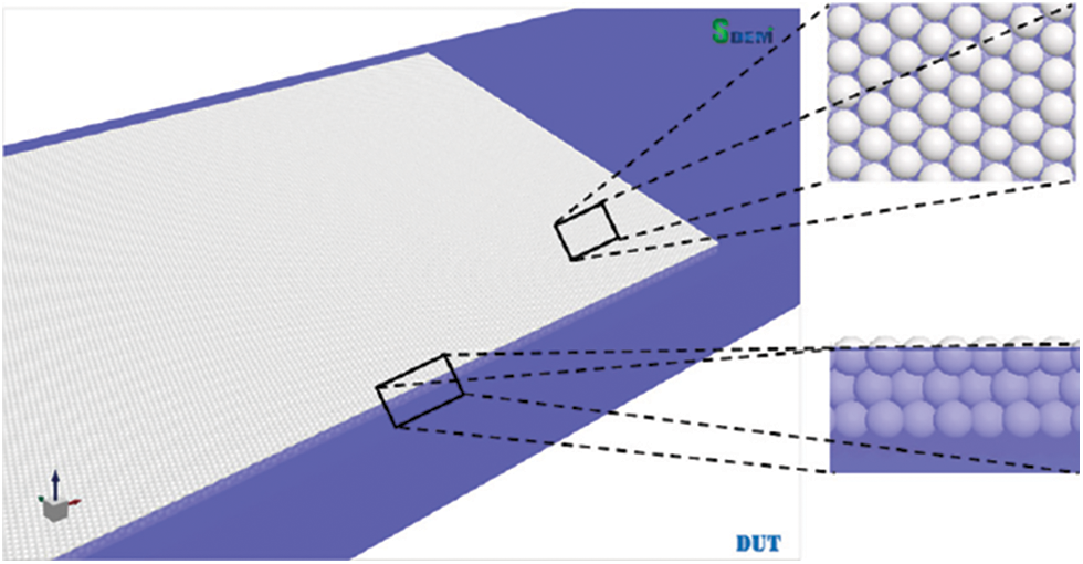
Figure 2: Level ice constructed by bonded spherical elements

The DEM parameters should be calibrated using relevant numerical mechanical tests to simulate the mechanical behaviors of level ice precisely. Based on the uniaxial compression and three-point bending tests of sea ice, the relationship between the DEM parameters and macroscopic mechanical parameters of level ice was established, considering the size effect [16,26]:

σb=σf/(1.77−1.81e−L/D4.78)(6)

μ=0.23σc/σf−0.5(7)

In Eqs. (6) and (7), σb is the cohesive strength, σf is the flexible strength, σc is the compression strength, L is the level ice thickness, and D is the spherical element diameter.

The model has been used to simulate the interaction between level ice and fixed structures such as the conical structure [27] and the vertical structure [28]. The comparison between the numerical results and the experimental results validated the rationality of the level model to simulate the interaction between level ice and various structures.

2.3 The Discrete Element Method of Mooring Lines

The DEM model of the mooring line is composed of a string of spherical elements, as shown in Fig. 3. In the bonded model of mooring lines, the bending stiffness is neglected, and the jointed elements behave like truss elements. Contrary to the level ice model, the main parameters in DEM for mooring lines are directly defined as the physical parameters of the mooring line. Catenary test and towed tests were simulated and compared with the FEM results and physical experiments to verify the accuracy of the DEM model.

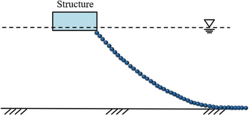
Figure 3: DEM model of mooring line

In the catenary test, the two ends of a stretchable mooring line are fixed in the direction of a slope angle of 45∘. The main computational parameters are listed in Table 1. The DEM model was used to simulate the equilibrium position and tension of the mooring line, and the results were compared with the nonlinear FEM results [29], as shown in Fig. 4. Both the curve shape and the tension distribution of the mooring line in the equilibrium position obtained through DEM simulations were almost in exactly agreement with the results of Kim et al. [29]. The elongation of the mooring line was significant, inducing a tension relaxation in the middle part of the mooring line. Therefore, the developed DEM has excellent ability to simulate the large deformation of mooring lines.

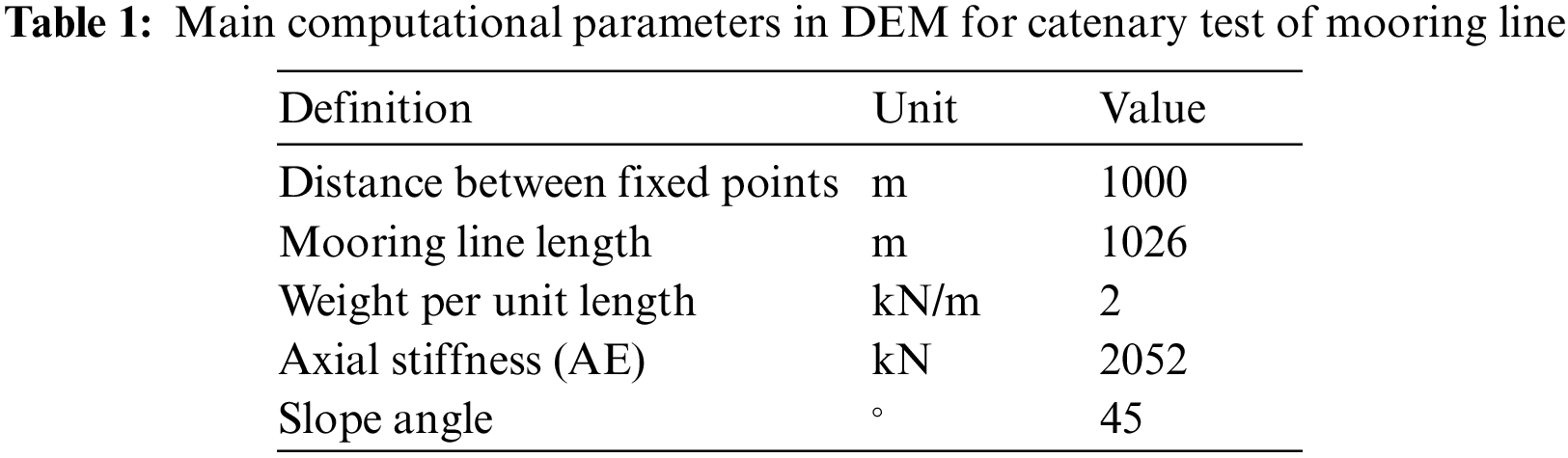
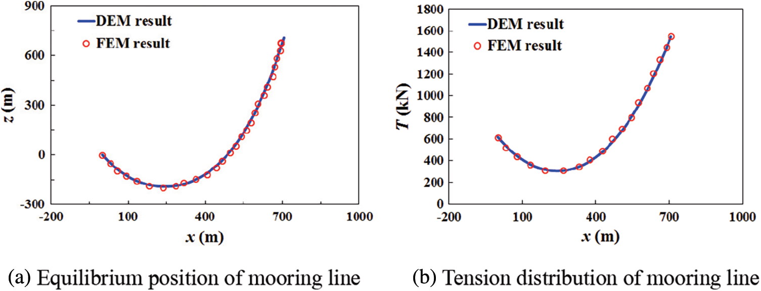
Figure 4: Comparison between DEM and FEM results of catenary test

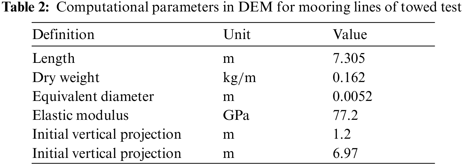
The DEM model was employed to calculate the dynamic response of the mooring line in the towed test [30]. The experimental system and DEM model are shown in Fig. 5, and the main parameters of the mooring line are listed in Table 2. The mooring line was towed by the top end which is in a simple harmonic surge with amplitude of 75 mm and period of 1.58 s. The motion of the marker located at 0.8m from the top-end of the mooring line was recorded in the test.

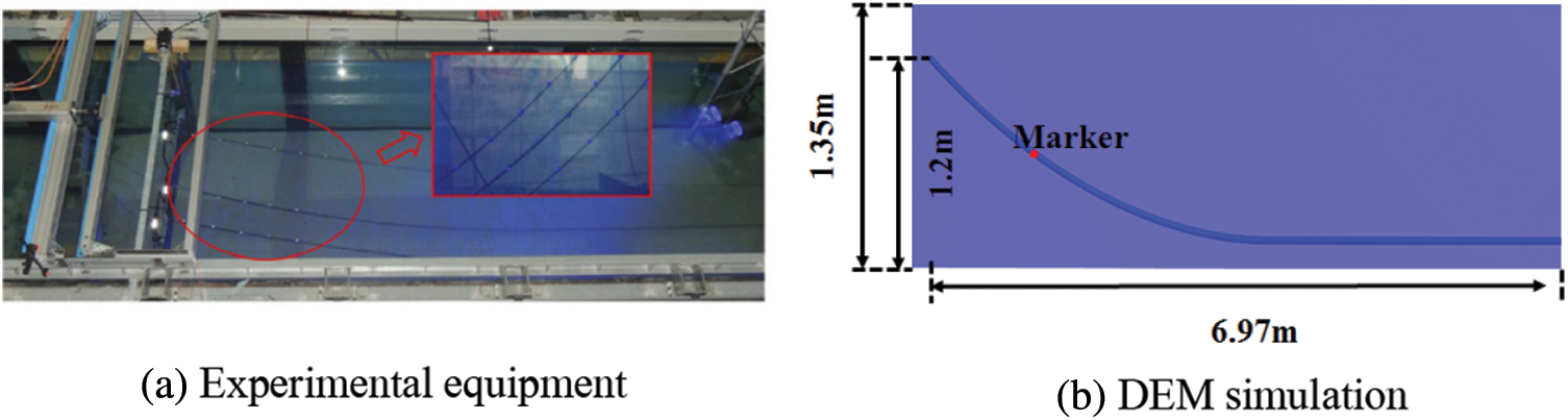
Figure 5: Mooring line in towed experiment and DEM simulation

The energy dissipation caused by hydrodynamic force has significant effect on dynamic behavior of the mooring line. The modified Morison formula [31] is employed to simulate the hydrodynamic force on a DEM element, as Eq. (8):

f→d=12CdD2ρ|v→r|v→r+14CaπD3ρa→rn+14πD3ρa→sn(8)

where D is the element diameter, ρ is the density of the fluid, Cd and Ca are the drag coefficient and added mass coefficient, respectively, v→r and a→rn are the relative velocity and normal acceleration of the fluid acting on the element, and a→sn is the normal acceleration of the fluid.

The calculation results were plotted compared with experimental results, as shown in Fig. 6. The calculated top-tension curve was consistent with the experimental data. The minimum tension, period and the asymmetry within a cycle induced by dynamic response of the mooring line are all consistent, but the maximum tension is slightly higher than the experimental value. Furthermore, the vertical motion of the marker was also compared. Overall, the vertical displacement is smaller than the experiment result, with a difference of less than 8%. Considering that the drag coefficient Cd is estimated according to Reynolds number, the error is reasonable. Hence, the DEM model is suitable to simulate dynamic response of mooring line.

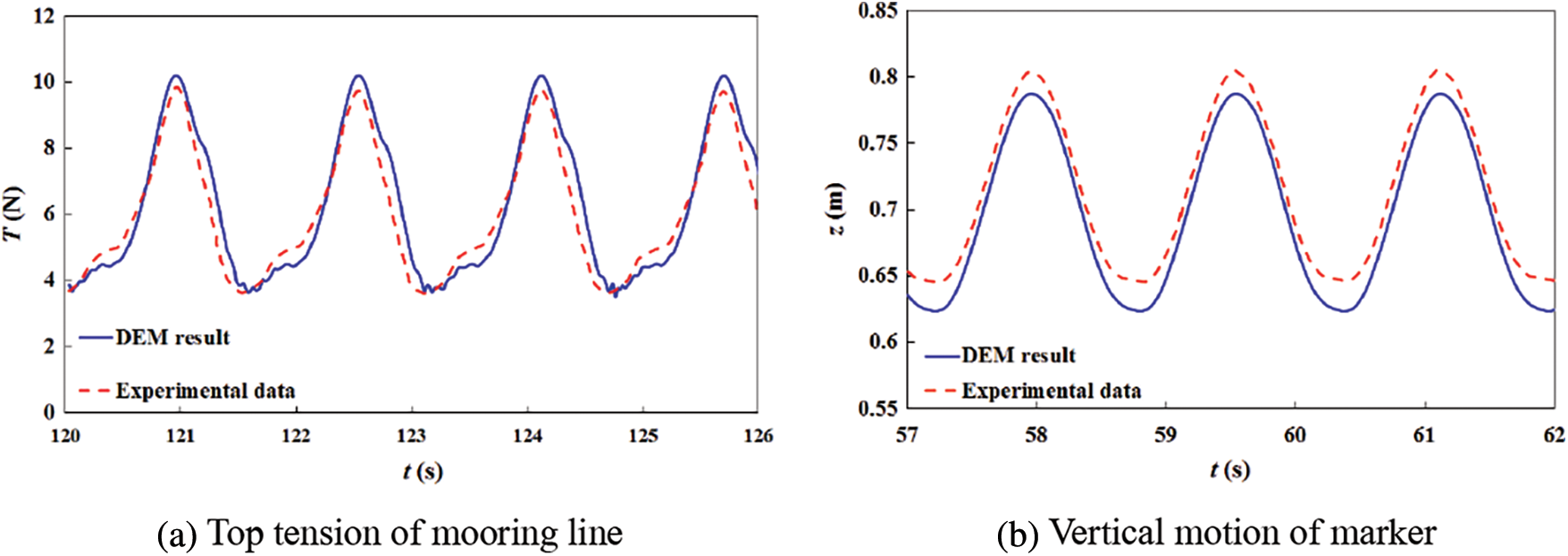
Figure 6: Comparison between DEM and experimental results of towed test

3  DEM Simulation of Interaction between Level Ice and Moored Semi-Submersible Structure

Based on the established DEM models of level ice and mooring lines, we adopted a moored semi-submersible structure to simulate its interaction with level ice. The platform with ice-resistant slope in the bow and stern mainly consisted of a hull and braces as Fig. 7; the platform was modeled as a rigid body with six degrees of freedom.

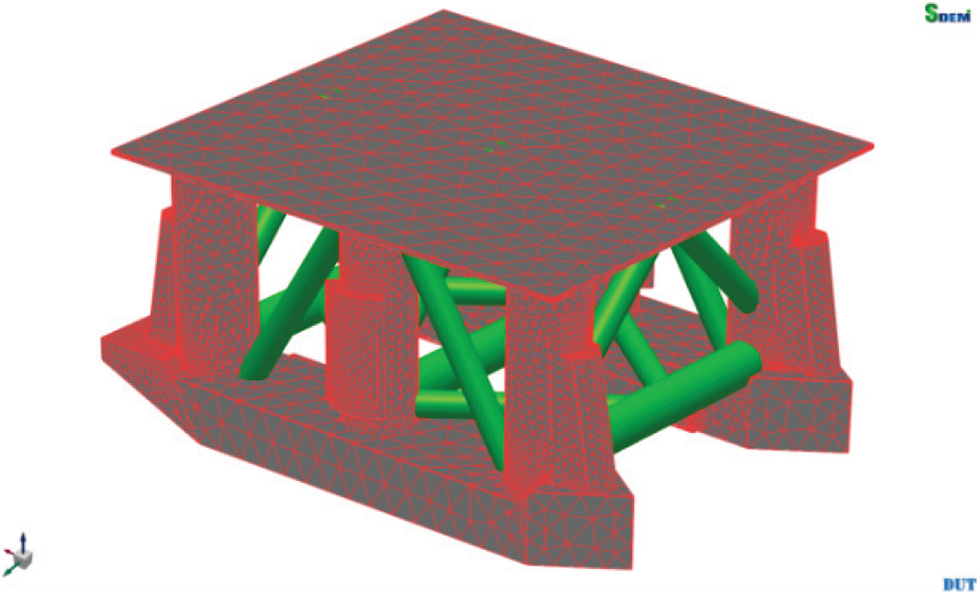
Figure 7: Semi-submersible structure in DEM simulation

3.1 Coupled Dynamic Equation of Moored Structure

The dynamic equation of a semi-submersible structure in the time domain is established according to the Cummins’ method [32]. The equation can be expressed as Eq. (9):

[MB+Madd(∞)]u¨+∫0t∫0∞2πC(ω)cos⁡[ω(t−τ)]dωu˙(τ)dτ+FB+FD=F(9)

where u is the motion vector including surge, sway, heave, roll, pitch and yaw, MB is the mass matrix, Madd(∞) is the added mass matrix when frequency ω=∞, FB is the buoyancy of the structure, C(ω) is the frequency-dependent damping coefficient according to which the potential damping is computed, FD is the quadratic damping term with FDi=Bi|u˙i|u˙i, F is the total extern load on the structure. In general, waves in the regions covered by level ice can be neglected. Therefore, we only considered the current drag force fc, ice load fi, and the mooring force fm to determine the global force on the semi-submersible structure. Therefore, the global force can be written as Eq. (10):

F=fc+fi+fm(10)

To simulate the rotation of the structure, a quaternion q was adopted to represent the global posture of the structure. The transition between q˙ and the rotation speed ωB in the local coordinate system fixed with the structure is expressed as Eq. (11):

[q˙0q˙1q˙2q˙3]=12[q0−q1−q2−q3q1q0−q3q2q2q3q0−q1q3−q2q1q0][0ωxBωyBωzB](11)

3.2 Numerical Simulation of Buoyancy of Semi-Submersible Structure

Buoyancy is the main component of restoring force and has significant effects on the stiffness of the dynamic system. Thus, the buoyancy of a structure was calculated based on the instantaneous submerged volume of the structure in every time step. For the hull composed of triangular elements (Fig. 7), the submerged volume is the sum of volume of the tetrahedron elements constructed by a reference pointin the water level and a submerged triangle area as Fig. 8. The volume of a tetrahedron element is given as Eq. (12):

Vi=13SiO⋅n(12)

where Si is the area of the triangular elements, O is the vector from the reference point O in the water level to an arbitrary point Oi in the triangular area, and n is the unit normal vector of the triangular elements.

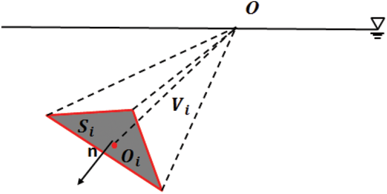
Figure 8: Tetrahedron element composed of reference point and triangle hull element

A numerical method was developed for simulating the buoyancy acting on the bracings. Each bracing is uniformly discretized into n segments along the axis of the bracing, as shown in Fig. 9a. The buoyancy of the bracing is the sum of buoyancy of each segment as Eq. (13):

FB=ΔL∑1nρgAi(13)

where ΔL is the segment length, ρ is the density of seawater, and g is the acceleration due to gravity. The submerged cross-sectional area Ai of each segment is calculated as Eq. (14):

Ai={πR2(hcosθ)≤−R−(hcos⁡θ)R2−(hcos⁡θ)2+R2arccos⁡(hcos⁡θ)−R≤(hcos⁡θ)<R0(hcos⁡θ)≥R(14)

where R is the radius of the cross-sectional section, h is the height of the cross-sectional section circle relative to the water surface, θ is the inclination of the brace to the water surface, as shown in Fig. 9b.

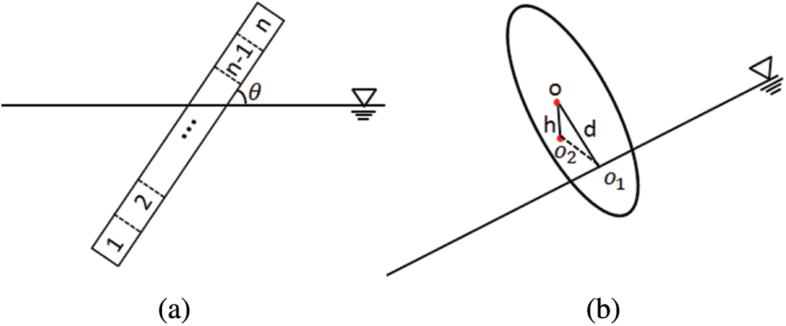
Figure 9: Sketch of a bracings intersecting with the water level

A free pitch oscillation test of the semi-submersible structure was simulated based on the proposed method for buoyancy calculations. The zero-up-crossing frequencies for different amplitudes of oscillation are as shown in Fig. 10. The resonance frequency the amplitude of oscillation increases with the amplitude of oscillation. Compared with the linear spring model, the proposed method can precisely simulate the nonlinear variation of the buoyancy during the pitch oscillation.

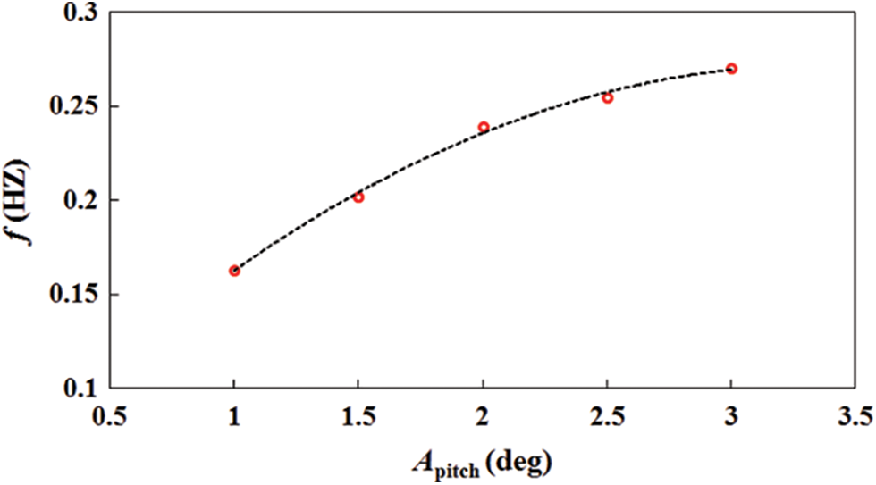
Figure 10: Zero-up-crossing frequencies for different oscillation amplitudes of the semi-submersible structure

4  DEM Simulations of Ice Load and Dynamic Behaviors of Semi-Submersible Structure

Based on the methods, we calculated the interaction between the semi-submersible structure and the level ice. The ice load and dynamic response of the structure were analyzed to validate reliability of the DEM method. Further, a series of simulations were performed to study the effect of ice thickness on the ice load and positioning ability of the semi-submersible structure.

4.1 Construction of Mooring System in Level Ice and Input Parameters

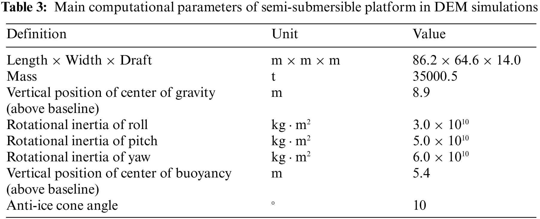
The moored semi-submersible platform concept was designed for drilling operations in the Barents sea. Considering that the maximum depth of the water is 600 m in the region, the depth was set to 400 m in the simulation. The interaction between mooring lines and the seafloor is calculated directly based on the contact law between spherical elements and the boundary of an arbitrary shape [33]. Here the seafloor was assumed to be a plane. The main parameters of the semi-submersible platform are shown in Table 3.

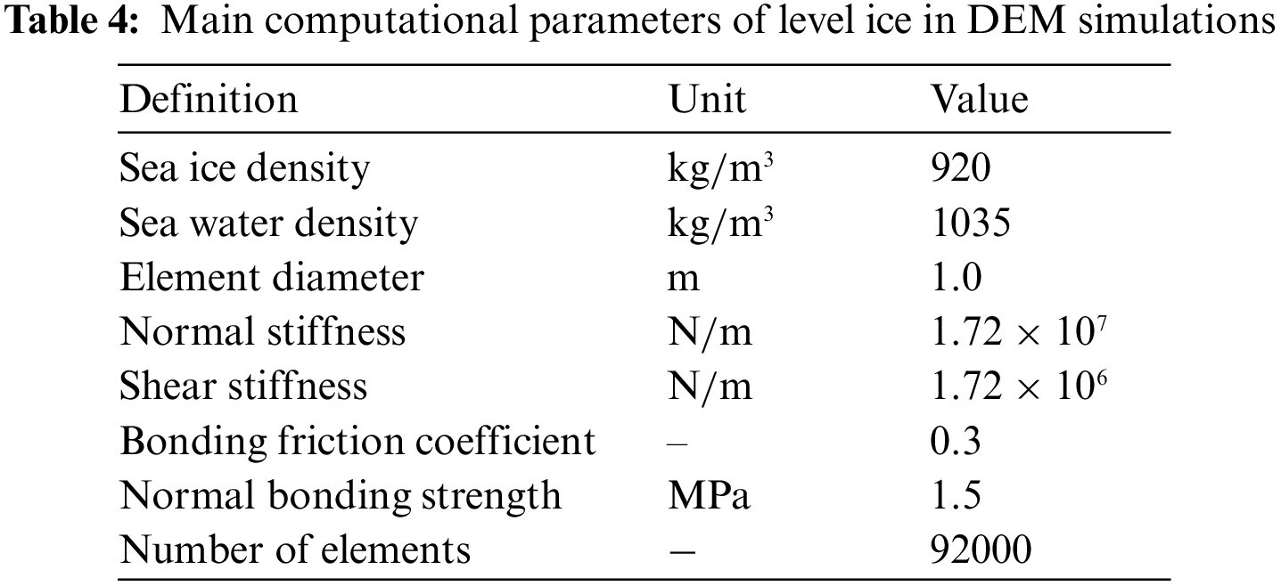
The level ice was assumed to be dragged by a current of 1 m/s with an ice area of 200 m × 400 m. The boundary of the level ice was set as a spring boundary, and the ice thickness is 1.0 m. The main DEM parameters are listed in Table 4.

The spread mooring system comprises 12 catenary mooring lines. The 12 mooring lines are grouped into four bundles stretching out in four directions symmetrically. Each bundle consisted of three mooring lines, and the angle between the adjacent lines is 5°, as shown in Fig. 11. Each mooring line consisted of three segments; the properties of the moorings are listed in Table 4, where EA is the axial stiffness and D is the equivalent diameter. The vertical distance between the fairlead and anchor point was 385 m and the tension of the mooring line was 221.7 kN.

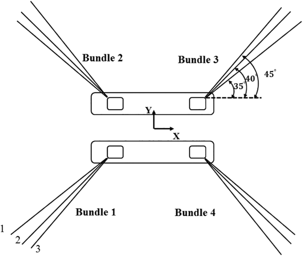
Figure 11: Schematic of mooring line arrangement of semi-submersible structure

The simulating time duration was set as 200 s to ensure the stability of the result and meanwhile, avoid the influence of the boundary of the level ice. According the wave propagation theory and related parameters of the DEM elements, the time step was set to be 10−5 s.

4.2 Ice Load and Mooring Load Simulated Using DEM

Fig. 12 shows four phases of the interaction between the level ice and moored semi-submersible structure: (a) initial contact, (b) equilibrium position, (c) drift motion, and (d) sea ice removal. At the initial stage, the level ice impacted the semi-submersible structure, forcing the structure to move. The semi-submersible structure is derived by the level ice to equilibrium point (14.7 m in the x-direction) in a nearly constant velocity, as shown in Fig. 13. After arriving at the equilibrium point, the structure started to vibrate periodically due to the coupled action of the ice load and mooring force. The level ice acted on the ice-resistant cone of the bow in a mixed failure mode of crushing and bending failures. Finally, the broken ice flowed through the semi-submersible structure without an obvious jam in front of the ice-resistant cone or among the braces.

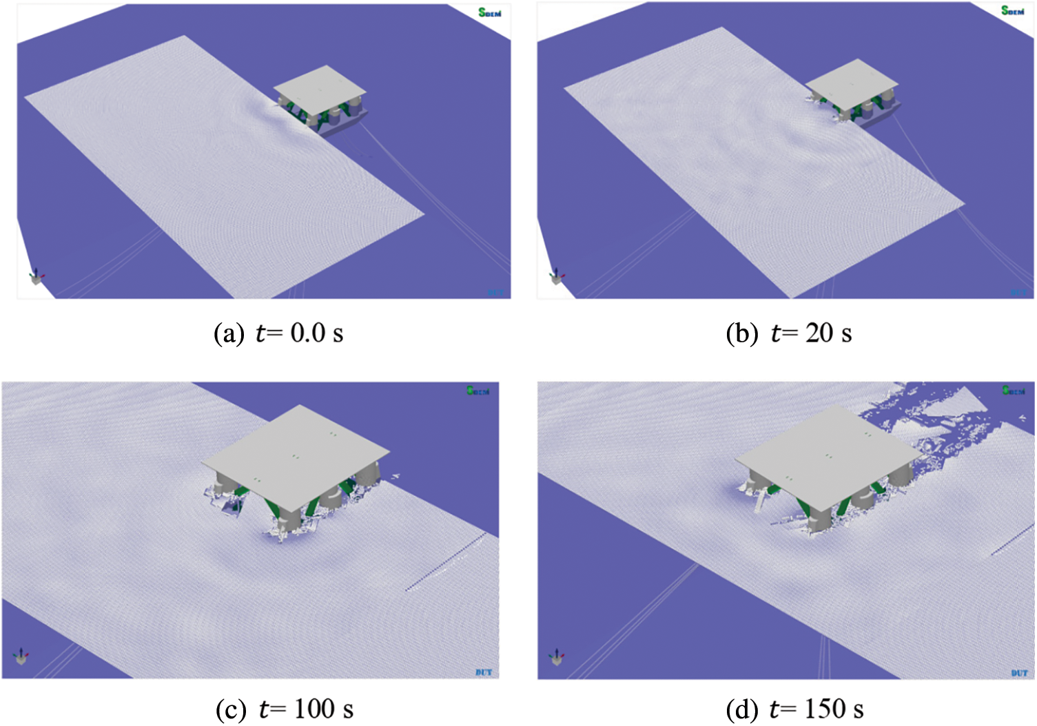
Figure 12: Interaction between level ice and semi-submersible structure simulated using DEM

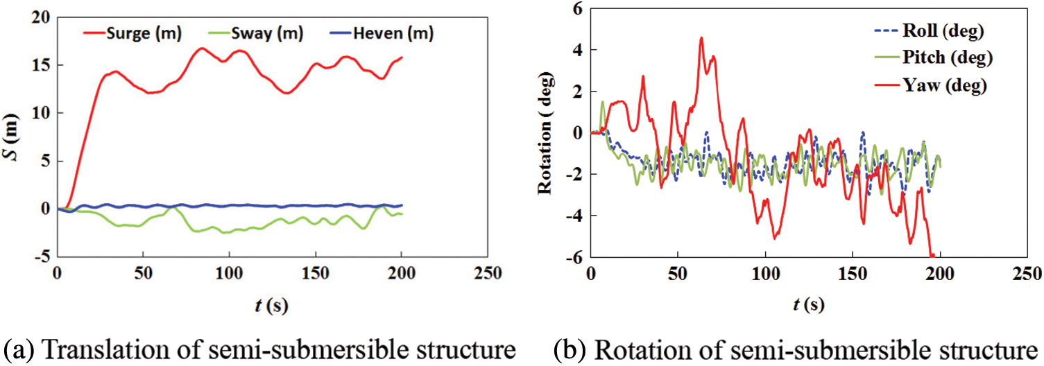
Figure 13: Dynamic motion of semi-submersible structure under ice load

The cone angle and dynamic friction angle of the ice-resistant structure were 10∘ and 26.5∘, respectively. According to the theory of Croasdale [34], only the crushing failure of the level ice occurs when the cone angle is less than the dynamic friction angle for a fixed cone. However, the mixed failure mode was observed in the simulation results, indicating that the dynamic response of the structure has an effect on failure mode of the level ice.

The amplitudes of surge, sway and heave are respectively 17.3, 3.6 and 0.2 m, respectively, and the maximum horizontal offset were less than 5% of the water depth (Fig. 13). Obviously, the mooring system satisfied the API 2SK requirements for station-keeping of the mooring structure. For the rotation, the amplitudes of the roll, pitch and yaw were 3.2∘, 2.6∘ and 5.9∘, respectively. The amplitude of the yaw was significantly greater than the amplitudes of the roll and pitch, whereas the frequencies of roll and pitch were higher than that of the yaw. The amplitude of the yaw significantly influenced on the interaction angle between the level ice and the semi-submersible structure, which may reduce the effect of ice-resistant structure. Therefore, it is essential to optimize the mooring system to constrain the yaw motion.

Fig. 14 shows the time history of ice load on the semi-submersible structure. The force in x-direction was the main load, greater than the loads in the other two directions. The maximum value of the load in x-direction was 30.1 kN. The ice load curve in the y-direction indicated apparent non-simultaneous failures of the level ice, which was also observed during the model test of the interaction between the level ice and semi-submersible structure [5]. The load in z direction was small, which shows that the crushing failure was the main failure mode in the ice-structure interaction.

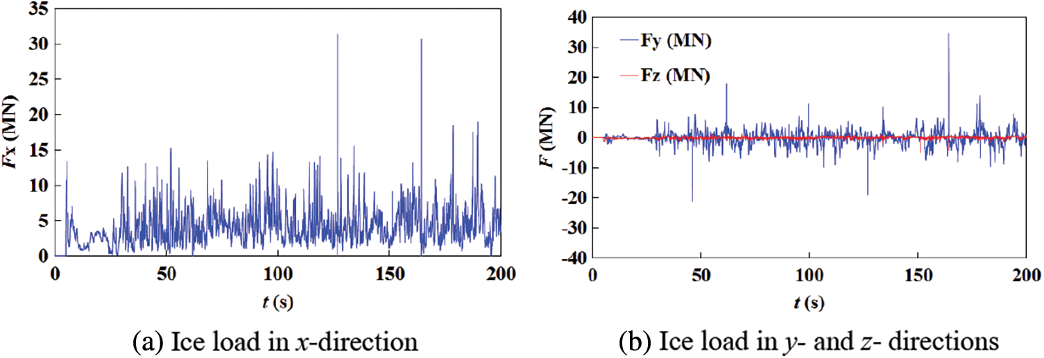
Figure 14: Time history of ice load on the semi-submersible structure simulated using DEM

The load on the semi-submersible structure without the conical ice-resistant structure can be estimated with the ISO formula [35]:

Fh=CRhD(hh1)n(Dh)m(15)

In Eq. (15), CR=1.5MPa; h1=1m; h is the ice thickness; D is the equivalent diameter of the columns of semi-submersible structure; n=−0.5+h/5; m=−0.16. The ISO result of the ice load on the semi-submersible structure was 40.1 kN. The comparison of the ISO result and the DEM result showed the conical ice breaking structure reduced the ice load by about 30%. As the ISO result is generally conservative, the DEM result was reasonable.

Fig. 15 shows the mooring forces of four mooring lines in different bundles in x-direction. As the semi-submersible structure moved to the equilibrium position, the mooring lines in Bundle 1 and 2 were tightened gradually, whereas those in Bundles 3 and 4 gradually relaxed. Subsequently, all the mooring lines started to vibrate. The overall trend of the mooring force in Bundle 1 and Bundle 2 followed the low-frequency drift (as Fig. 13a) of the semi-submersible structure. On the contrary, the rotation of the semi-submersible structure (as Fig. 13b) and wave transmission along the mooring lines induced high- frequency oscillation of the mooring force.

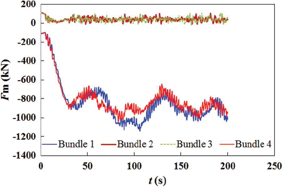
Figure 15: Mooring forces of mooring lines in different bundles in x-direction

The maximum tension of the mooring lines is a important critical design parameter for moored structures, according to API 2SK [36]. Fig. 16 shows the history of the maximum tension in the three mooring lines in Bundle 1. The tensions of the three mooring lines were somewhat consistent. The maximum tension of the mooring lines is 1.9 MN, which is significantly lower than the fracture strength 4.4 MN. The mooring system satisfied the recommended safety factor of 1.67.

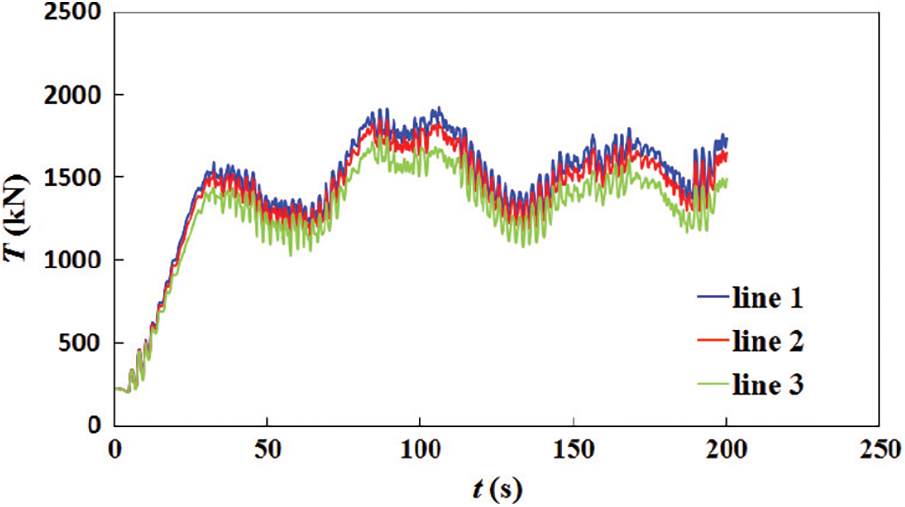
Figure 16: Tension of mooring lines in Bundle 1 in x-direction

4.3 Influence of Ice Thickness on Ice Load and Mooring Load

Ice thickness is a key parameter in ocean engineering design for ice-covered regions. A series of numerical calculations were conducted to analysis the effect of ice thickness on the ice load of the moored semi-submerged structure. The ice thickness ranged from 1 to 1.6 m in intervals of 0.2 m in the simulation. The other parameters of the semi-submerged structure, level ice and mooring system are listed in Tables 3–5, respectively.

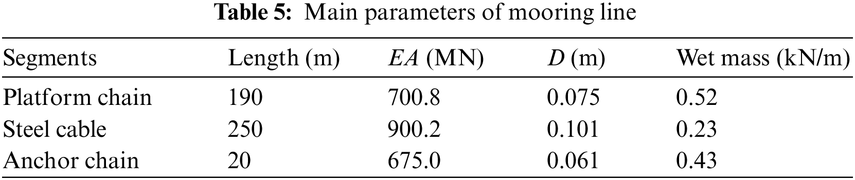
Fig. 17 shows the maximum values of the ice load in x- and z-directions in different ice thicknesses. It is noted that the maximum ice load in the both directions increases linearly with the increase of the ice thickness. The relationship was also observed in experimental results of other structures, such as Kulluk [1] and moored tankers [2]. When the ice thickness varied from 1 to 1.6 m, the maximum value of the ice load in x-direction increased about 70%. The ratio of the maximum value of the ice load in z-direction to that in x-direction decreased steadily. This may be because the crushing failure became more dominant in the mixed fracture mode of the level ice as the ice thickness increased.

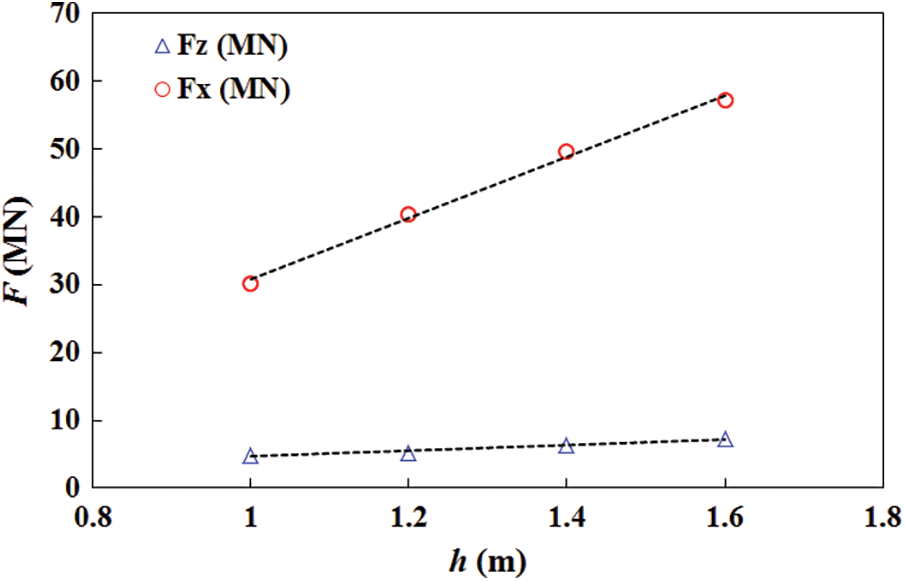
Figure 17: Maximum ice loads of semi-submersible structure for different ice thicknesses

Fig. 18 shows the maximum values of the restoring force of the mooring system in different ice thickness and the corresponding offsets of the semi-submersible structure. The maximum restoring force increased linearly from 7.2 to 11.3 MN as the ice thickness increased. Due to the dynamic effect, the maximum restoring force was far lower than the maximum ice load in the x-direction. The maximum offset smax increased linearly from 17.6 to 23.8 m, and the mean offset smax increased linearly from 14.6 to 18.7 m. It is of concern that the offset reached 15.9 m, when the ice thickness was 1.2 m. That means level ice with a thickness of more than 1.2 m will induce a mean offset of the semi-submersible structure exceeding the design criteria [36]. Hence, a greater pretension or a dynamic assisting system should be considered in the design of the mooring system for the thick level ice.

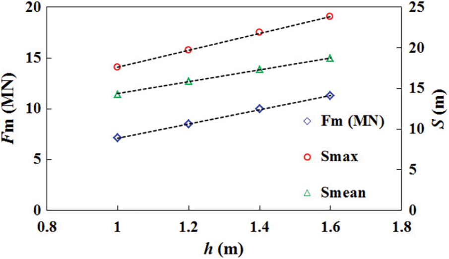
Figure 18: Maximum restoring forces of mooring system and offsets of semi-submersible structure for different ice thicknesses

5  Conclusions

A DEM method was established in the study to accomplish coupled calculations of the ice load and mooring force of moored structures in level ice. The DEM models of the level ice and mooring lines were based on spherical elements with different parallel bonding models. A catenary test and a towed test were simulated to validate the accuracy of the mooring line model. The dynamic response of a semi-submersible structure was simulated using the proposed DEM model. In the simulations, the buoyancy was calculated based on the instantaneous submerged volume of the semi-submersible structure to model the nonlinear dynamic characteristics of the structure. The comparison between the DEM result and the ISO result validated the reasonability of the DEM method to simulate the ice load and mooring force of a moored structure in level ice.

The DEM results demonstrated the dynamic behavior of the semi-submersible structure significantly influenced the failure mode of level ice. The surge and yaw motion were the most critical among the motions of the semi-submersible structure in level ice with six degrees of freedom. The tension of the mooring lines mainly depended on the surge motion of the structure.

The influences of the ice thickness on the ice load and the mooring force were also analyzed. The results shown the maxim values of the ice load and mooring force were all in a linear positive correlation with the ice thickness. The mean and maximum offset also increased evidently as the ice thickness increased. For the mooring system analyzed in this paper, the mean offset exceeded the design criteria for the level ice thicker than 1.2 m. The mooring system should be optimized for the thick level ice in future studies.

Funding Statement: This study is financially supported by the National Natural Science Foundation of China (Grant Nos. 11872136, U20A20327 and 42176241).

Conflicts of Interest: The authors declare that they have no conflicts of interest to report regarding the present study.

This work is licensed under a Creative Commons Attribution 4.0 International License, which permits unrestricted use, distribution, and reproduction in any medium, provided the original work is properly cited.