Computer Modeling in Engineering & Sciences

DOI: 10.32604/cmes.2022.019828

ARTICLE

A Fast Element-Free Galerkin Method for 3D Elasticity Problems

Zhijuan Meng1, Yanan Fang1 and Yumin Cheng2,*

1School of Applied Science, Taiyuan University of Science and Technology, Taiyuan, 030024, China
2Shanghai Key Laboratory of Mechanics in Energy Engineering, Shanghai Institute of Applied Mathematics and Mechanics, School of Mechanics and Engineering Science, Shanghai University, Shanghai, 200072, China
*Corresponding Author: Yumin Cheng. Email: ymcheng@shu.edu.cn
Received: 18 October 2021; Accepted: 15 December 2021

1  Introduction

The 3D elasticity problem is one of the typical mechanical problems in engineering. Because of the complexity of this type of problems, it is difficult to get the analytical solution when the problems are defined in complicated domains. Therefore, the study of the numerical method for 3D elasticity has important theoretical and practical significance. At present, lots of methods have been applied to simulate elasticity problems, such as the finite element method (FEM) [1], finite difference method [2], boundary element method (BEM) [3] and meshless method [4–7].

The meshless method has been an important numerical method for scientific and engineering problems [8–13]. When using the meshless method to solve problems, only discrete nodes need to be distributed in the problem domain and on the boundary. Furthermore, different problems can flexibly distribute the quantity of nodes according to the characteristics. Therefore, the meshless method has good adaptability and high calculation accuracy. It is more suitable for solving those complex problems, for example, crack growth, super large transfiguration and high-speed collision.

The IEFG method is one of the important meshless methods. The shape function is constructed using the improved moving least-squares (IMLS) approximation [14,15]. The IMLS approximation is based on the ordinary least-squares method which has high accuracy and has been applied in various fields [16–18]. Furthermore, the basis functions of the IMLS method are weighted orthogonally. Compared it with the classical element-free Galerkin method, the IEFG method has fewer coefficients, and the computational speed is faster. Zhang et al. used the IEFG method to simulate 3D heat conduction problems [19], 3D potential problems [20] and 3D wave propagation [21]. Ma et al. used the IEFG method to simulate groundwater pollution prevention and control and its application in fluid flow [22]. Peng et al. used it to simulate 3D viscoelasticity problems [23]. Zheng et al. used it to simulate diffusional drug release problems [24]. Yu et al. used it to simulate three-dimensional elastoplasticity problems [25]. Liu et al. used it to simulate elastic large deformation problems [26] and inhomogeneous swelling of polymer gels [27]. Cai et al. used it to simulate elastoplasticity large deformation problems [28]. Wu et al. used it to simulate the elasticity [29]. Zou et al. used it to simulate fracture problems of airport pavement [30]. Cheng et al. used it to simulate the unsteady Schrödinger equation [31]. Cheng et al. used it to simulate nonlinear large deformation [32]. However, for 3D problems, the CPU running time of IEFG method is still long. To improve the computational efficiency, the DSM is introduced to complete the 3D problems.

Using the DSM, the 3D problem can be changed into a series of interrelated 2D problems. Li et al. first chose the DSM to solve the 3D linearly elastic shell [33] and incompressible Navier-Stokes equations [34]. Hou et al. solved a 3D elliptic equation appling the dimension splitting algorithm [35]. Ter Maten EJW applied the splitting method to solve fourth order partial differential equations [36]. Bragin et al. applied dimension splitting to analyze the conservation law [37]. Meng et al. presented the dimension splitting element-free Galerkin method to simulate 3D potential problems [38], 3D wave equations [39], 3D advection-diffusion problems [40] and 3D heat conduction problems [41]. Cheng et al. used the dimension splitting and improved complex variable element-free Galerkin method to simulate 3D problems [42–45]. Wu et al. applied the interpolating dimension splitting element-free Galerkin method to simulate 3D heat conduction and 3D potential problems [46,47]. Peng et al. combined the dimension splitting method and reproduce kernel particle method [48–50] to simulate some classical 3D problems [51–53]. The results of references [38–53] show that the computational efficiency can be greatly improved by the DSM.

In this paper, the FEFG method for 3D elasticity is proposed. The key problem is transforming a 3D elasticity into a series of interrelated 2D elasticities using dimension splitting. Then the 2D problems are simulated with the IEFG method and FDM is chosen in the splitting direction. The final discretized system equations of the 3D elasticity problem are obtained. Some specific examples are provided to illustrate the high accuracy and efficiency of the FEFG method for 3D elasticity by comparing the results of the FEFG method with ones of the IEFG method and analytical solutions.

2  The IMLS Approximation

The trial function of the moving Least-squares (MLS) method approximation is

(1)

where are basis functions, m is the number of basic functions. are the coefficients of .

The form of is often given according to the characteristics of the problem.

To minimize the local approximation error, the coefficients are calculated by the weighted least square method. Let the functional

(2)

where means the weight function, are points whose influence domain include ,

(3)

(4)

(5)

(6)

In order to obtain , from

(7)

we have

(8)

where

(9)

(10)

Finally, we can obtain the trial function as

(11)

where represents the shape function. We have

(12)

(13)

For the IMLS method, a set of orthogonal functions is chosen as the basis function. The ill conditioned or singular equations can be avoided. The inverse of the matrix can be obtained directly, which improves the calculation efficiency.

The orthogonal basis functions can be structured by the Schmidt method. For example, basis functions

(14)

are orthogonalized to the following orthogonal basis functions.

(15)

Eq. (7) can be expressed as

(16)

If is a set of orthogonal functions, that is

(17)

Eq. (16) becomes to

(18)

We can simply have

(19)

Then

(20)

where

(21)

Substituting Eq. (19) into Eq. (11), we obtain

(22)

where mean the shape function, and

(23)

3  The FEFG Method for 3D Elasticity

The equilibrium equation of 3D elasticity is

(24)

(25)

(26)

with the boundary conditions

(27)

(28)

where mean the stress, mean the body force, mean the displacement, is the boundary of problem domain , and . mean the known displacement on , mean the known traction on , and is the unit external normal vector to .

Then, the elasticity problem composed of Eqs. (24) and (25) and the boundary conditions is solved by the FEFG method.

The 3D problem domain is divided into 2D subdomains along direction , which is chosen as the splitting direction, that is, 2D planes are inserted into . And the distance between two adjacent 2D sub-domains is . That is

(29)

where

(30)

(31)

For a fixed , Eqs. (24) and (25), the essential boundary conditions Eq. (27) and the natural boundary conditions Eq. (28) can be transformed as

(32)

(33)

with the boundary conditions

(34)

(35)

where mean the displacement in the 2D domain , mean the known displacement on , mean the known traction on , and , , mean the unit outward normal to boundary .

Applying the IEFG method to solve the 2D problem of Eqs. (32)–(35), the trial function at is related to the value at nodes whose domain of influence covers . It can be expressed as

(36)

where

(37)

(38)

The strain at any point in subdomain is

(39)

It can be written as

(40)

where

(41)

The stress at any point in subdomain is

(42)

For plane stress problems,

(43)

and for plane strain problems,

(44)

where E means Young's modulus, means Poisson's ratio, and means the elasticity matrix [54].

The penalty method is applied to apply the essential boundary conditions, and the weak form of the Galerkin integral of Eqs. (32)–(35) is

(45)

where

(46)

is the shear modulus, and

(47)

(48)

(49)

(50)

(51)

(52)

If is the displacement on along direction , , otherwise .

Eqs. (36), (40), (42) and (47) are substituted into Eq. (45). Then, we have

(53)

To get the solvable algebraic equations, all integrals in Eq. (53) need to be analyzed separately.

The first integral term in Eq. (53) is

(54)

where

(55)

The second integral term in Eq. (53) is

(56)

where

(57)

The third integral term in Eq. (53) is

(58)

where

(59)

The fourth integral term in Eq. (53) is

(60)

where

(61)

The fifth integral term in Eq. (53) is

(62)

where

(63)

The sixth integral term in Eq. (53) is

(64)

where

(65)

Substituting Eqs. (54), (56), (58) (60), (62) and (64) into Eq. (53), we obtain

(66)

For the is arbitrary, we let

(67)

where

(68)

(69)

In order to obtain the solution of Eq. (67), points are uniformly inserted along direction in domain . Let

(70)

(71)

(72)

(73)

(74)

Using the FDM in the splitting direction , we have

(75)

Then, Eq. (67) is written as

(76)

(77)

(78)

(79)

The matrix form of Eqs. (76)–(79) is

(80)

where

(81)

Let

(82)

(83)

(84)

Eq. (80) is simplified to

(85)

The solution of Eq. (85) is the numerical solution of the displacement in direction and at each node on the middle layer .

The boundary value problem composed of Eqs. (25) and (26) and the corresponding boundary conditions can also be solved by the FEFG method, and the numerical solutions of displacement in direction and at each node can be obtained. Finally, we can get the numerical solutions of Eqs. (24)–(28).

In this paper, the FEFG method is for isotropic materials. We think that the FEFG method can also solve 3D linear elasticity for anisotropic materials. As long as the constitutive equations of anisotropic materials are established, the FEFG method can be obtained. It can be used as our later research topic.

4  Numerical Examples

Four related numerical examples are calculated using the FEFG method. The outcomes under different penalty factors, scale parameters and node distributions of the FEFG method are studied. Through comparing the numerical outcomes of the FEFG method with those of the IEFG method, the superiority of the FEFG method for 3D elasticity problems can be found. We can find that the calculation efficiency of the FEFG method is much faster than the IEFG method and the calculation accuracy of the FEFG method is also high.

The relative error is defined as

(86)

where

(87)

4.1 Cube under Uniformly Distributed Load

The cube was subjected to a uniformly distributed load as shown in Fig. 1. The side length is 2 m. The distributed load is , the shear modulus is and Poisson's ratio is . The analytical solution of displacement is given as

(88)

(89)

(90)

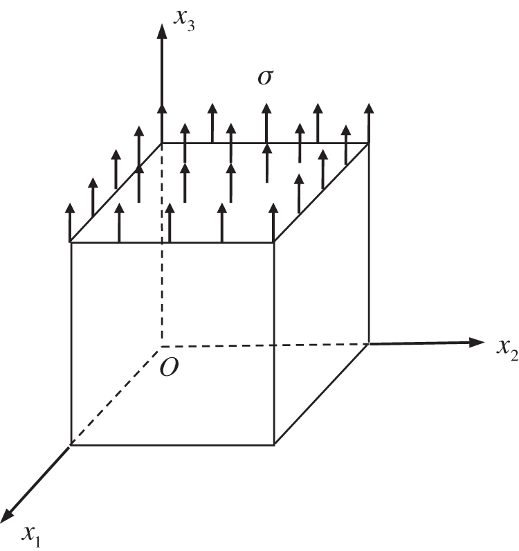
Figure 1: A cube under a uniformly distributed load

Using the IEFG method to solve this problem, 11 × 11 × 11 node distributions are selected, the influence domain factor , and the penalty factor . Then, the CPU running time is 12.78 s. The overall relative error is . The relative errors of the displacement in direction , and are , and , respectively.

Then, the FEFG method is used to solve this problem. Direction is chosen as the splitting direction. Nine planes are inserted along direction , and 11 × 11 nodes are evenly distributed on the plane . In addition, and . Then, the CPU running time is 0.64 s. The overall relative error is . The relative errors of the displacement in directions and are and , respectively. The parameter selection makes the FEFG method optimal.

Table 1 shows the calculation accuracies and CPU running times of the FEFG and IEFG methods when is different. 11 × 11 × 11 node distributions were selected. In order to achieve high calculation accuracies for every method, for the IEFG method and for the FEFG method.

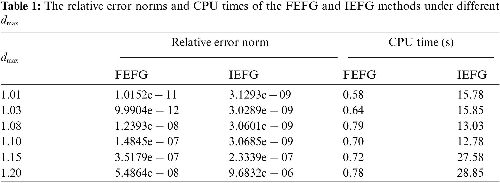
Fig. 2 shows that has great influence on the error. In this paper, we choose for the FEFG method.

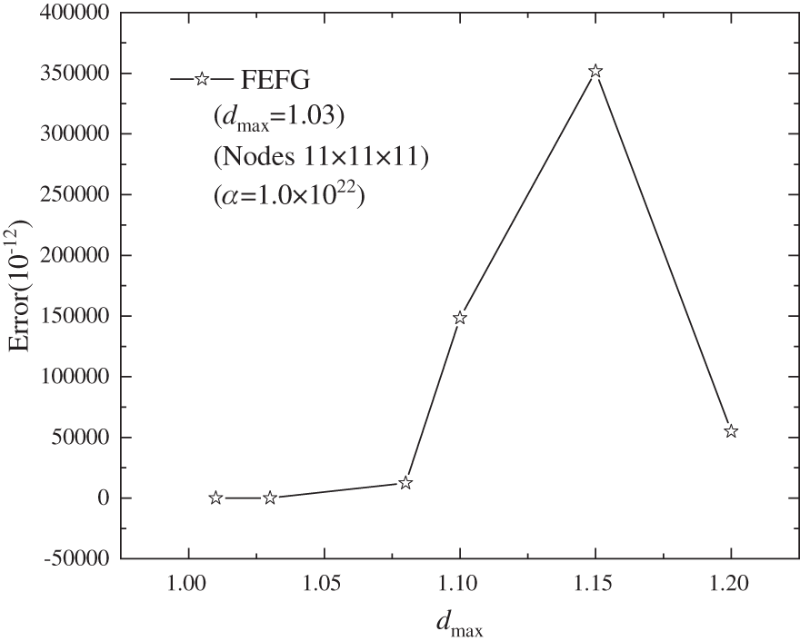
Figure 2: The error of the FEFG method with different

Table 2 shows the calculation accuracies and CPU running times of the FEFG and IEFG methods when the node distributions are different. We find that the calculation accuracies of the IEFG and FEFG method are both very high for this problem. However, the calculation time of the FEFG method is much shorter than that of the IEFG method. In this case, we set the node distribution is 11 × 11 × 11.

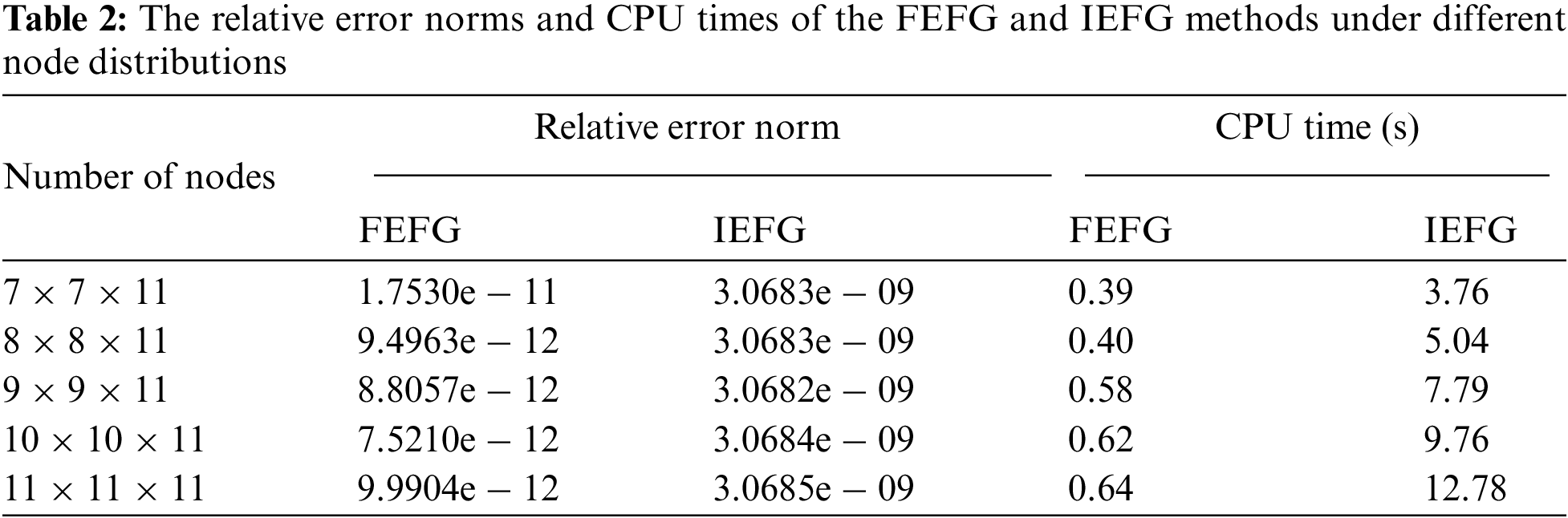
Table 3 illustrates the calculation accuracies and CPU running times of the FEFG method when the penalty factor is different. The has a great influence on the numerical results. Then the appropriate coefficient can be selected to obtain higher calculation accuracy. Fig. 3 illustrates the error of the FEFG method under different . In this paper, we choose for the FEFG method.

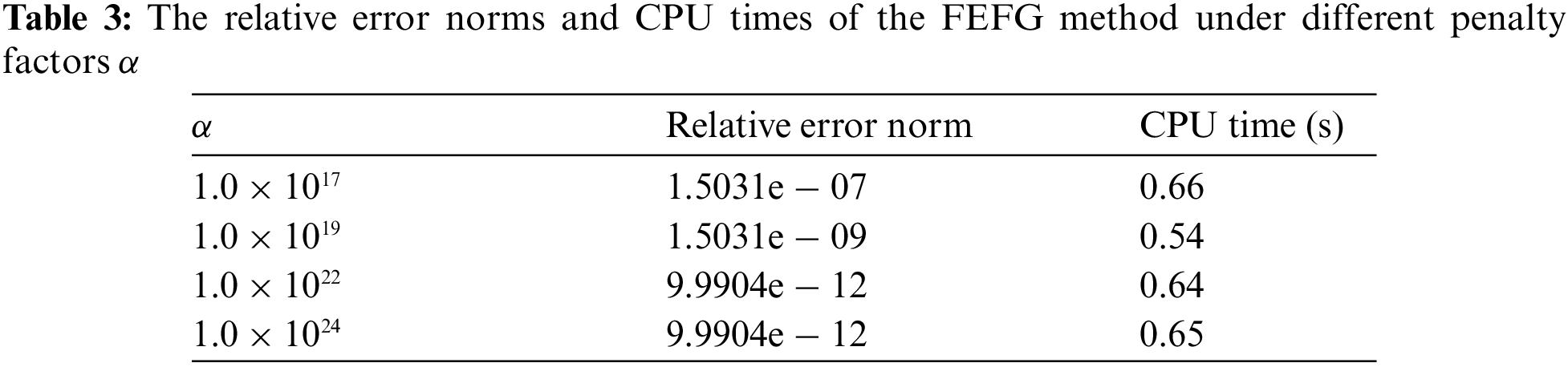
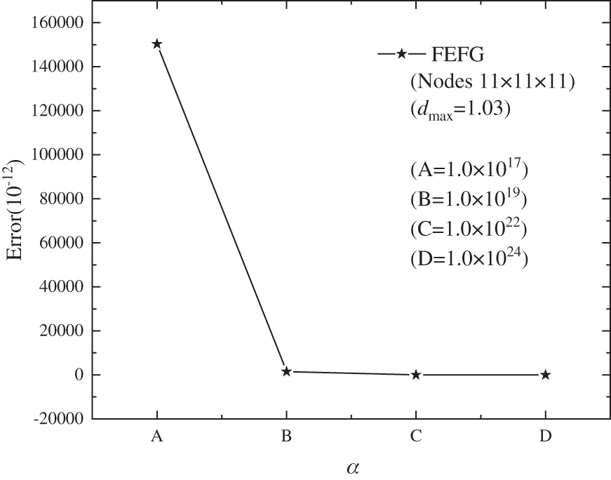
Figure 3: The error of the FEFG method is distributed with

Figs. 4–6 are the results of displacement , and of the FEFG method, IEFG method and analytical solution along direction , and , respectively. We find that the two methods are very consistent with the analytical results and the FEFG method is faster than the IEFG method.

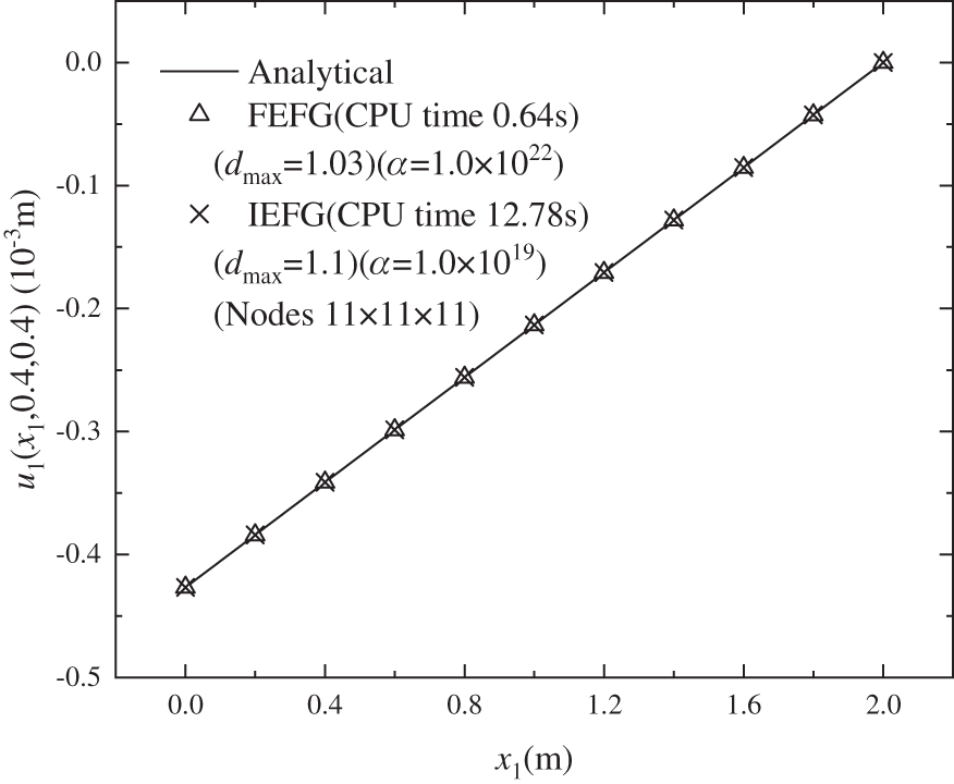
Figure 4: The distribution of the displacement along

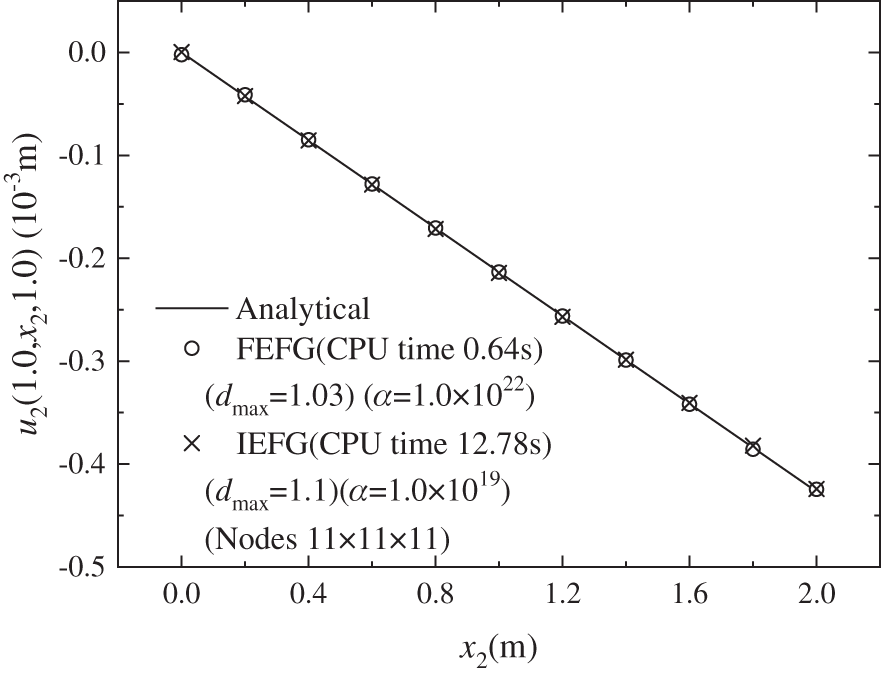
Figure 5: The distribution of the displacement along

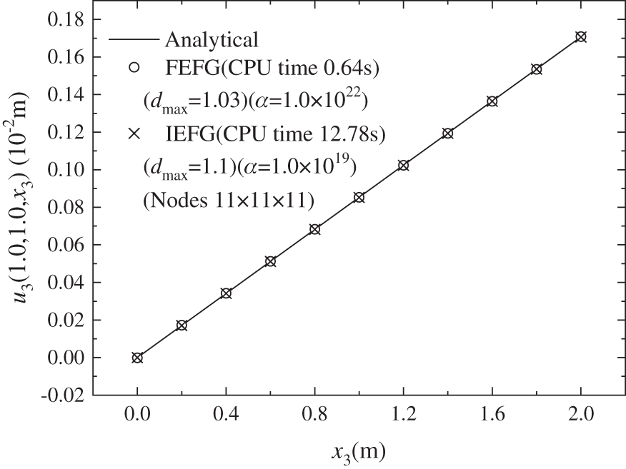
Figure 6: The distribution of the along

4.2 Prismatic Bar Considering Its Own Weight

Suppose the gravity of the bar per unit volume is as shown in Fig. 7. The body force are

(91)

(92)

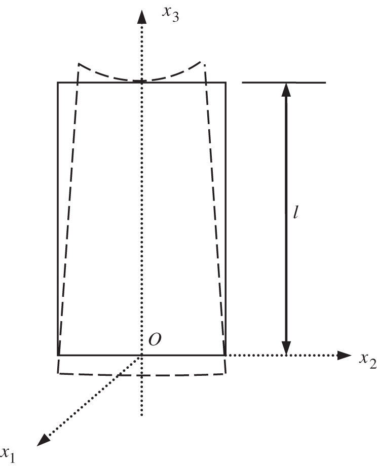
Figure 7: Prismatic bar

The stresses are

(93)

(94)

The geometrical size of the bar is , poisson's ratio is , density is and the Young's modulus is . The analytical solution of the displacement field is

(95)

(96)

(97)

Adopting the IEFG method to solve this problem, the node distribution is 5 × 5 × 11, , and . Then, the CPU running time is 44.53 s. The overall relative error is .

Next, the FEFG method is used to solve this problem. Direction is the splitting direction. Three planes are inserted along direction . On plane , 5 × 11 mesh nodes are selected evenly and , . Then, CPU running time is 0.38 s. The overall relative error is . It can be seen that the FEFG method can notably increase the computing efficiency.

Figs. 8–10 are comparison of displacements , and along direction , and by the FEFG and IEFG methods with analytical solutions. Fig. 11 is the calculation results of stress by the FEFG method, the IEFG method and the analytical solution along . We find that the two methods are very consistent with the analytical results and the FEFG method is faster than the IEFG method.

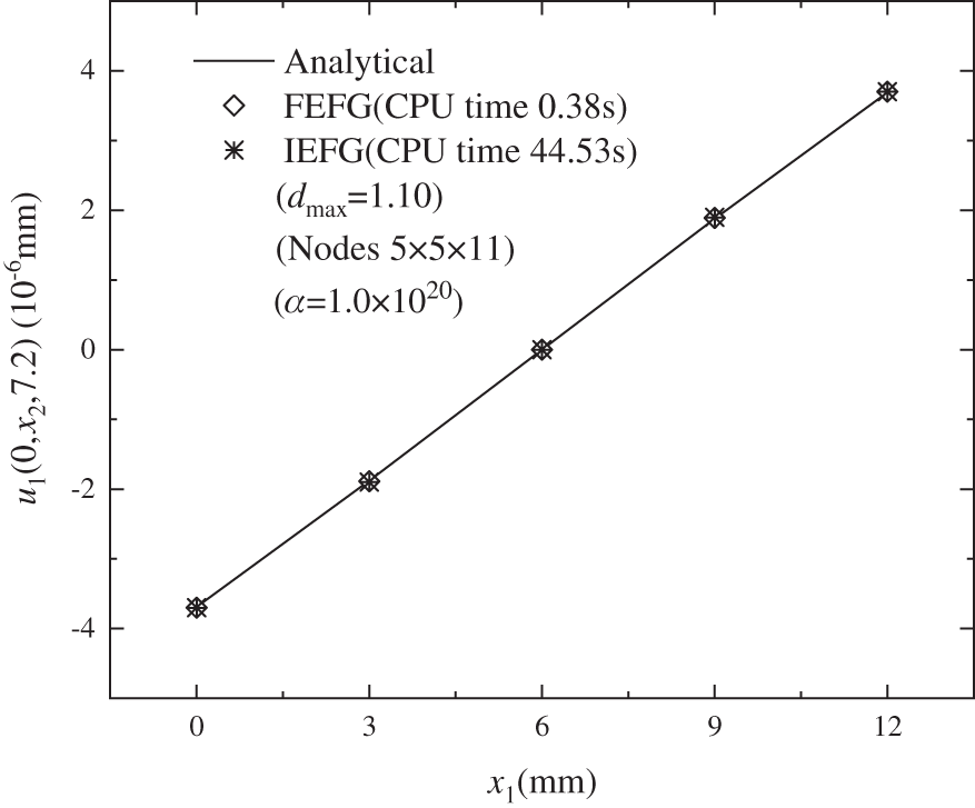
Figure 8: The distribution of displacement along

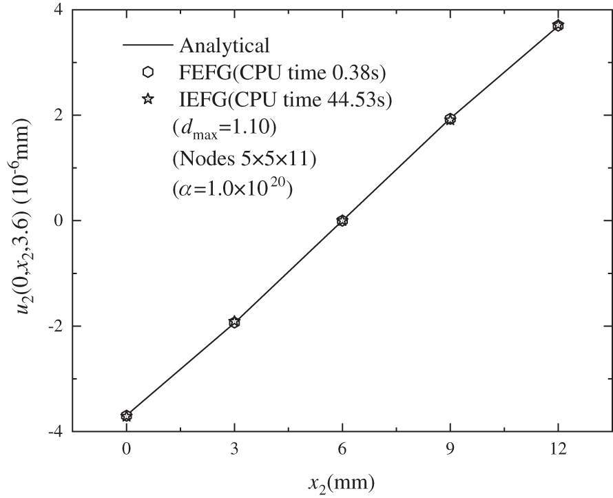
Figure 9: The distribution of displacement u2 along

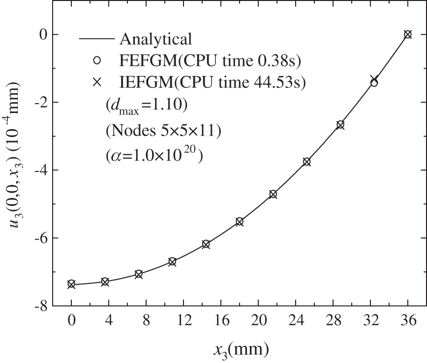
Figure 10: The distribution of displacement along

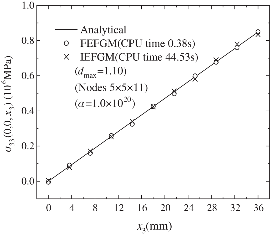
Figure 11: The distribution of normal stress along

Fig. 12 shows the relationship between stress and strain at point (0, 0, ) by the FEFG method, the IEFG method and the analytical solution. We can find that the numerical solutions agree well with the analytical solutions.

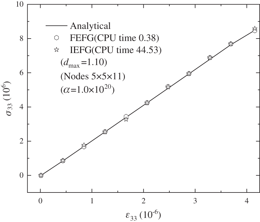
Figure 12: The effect of stress along strain

4.3 3D Semi-Infinite Solid

For a 3D semi-infinite solid in Fig. 13, is its boundary, and the displacement and stress are caused by a distributed load. The weight per unit volume is . The body forces are

(98)

(99)

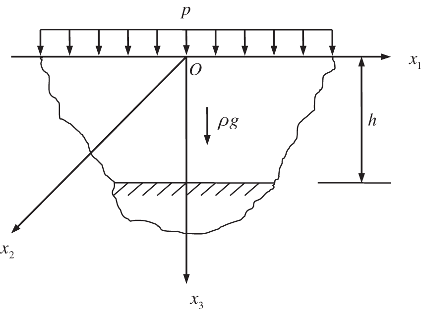
Figure 13: 3D semi-infinite solid

In addition, , , , and . Here, p is the ratio of the pressure per unit area in plane , is the density, v is the Poisson's ratio and E is the Young's modulus. The analytical results of this case are

(100)

(101)

(102)

(103)

After selecting a cuboid 300 meters long, 300 meters wide and 100 meters high, the IEFG method is used to solve this problem, and 6 × 6 × 9 mesh nodes are selected. , and . Then, the CPU running time is 5.75 s, and the overall relative error norm of and are 0.0982 and 0.1030, respectively.

Next, the FEFG method is selected to solve this problem. The direction is the splitting direction. Four planes are inserted along direction . On plane , 6 × 9 nodes are evenly distributed. In addition, , and . Then, the CPU running time is 0.38 s, and the overall relative error norm of and are 0.0575 and 0.0691, respectively. It can be seen that the FEFG method is much faster and more accurate than the IEFG method in solving the and of this case.

Table 4 illustrates the calculation accuracies and CPU running times of the FEFG method and the IEFG method when is different. In addition, the node distribution is 6 × 6 × 9, and . It can be seen that the IEFG method and FEFG method both have better computational precision, as shown in . For this case, we let .

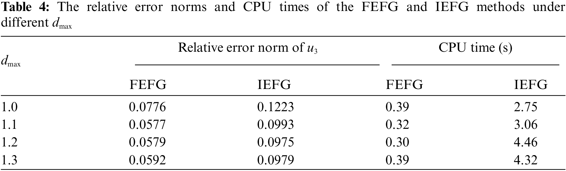
Table 5 illustrates the calculation accuracies and CPU running times of the FEFG with different node distributions. It can be seen that the FEFG method is convergent. For this problem, we choose the integral node distribution is 6 × 6 × 9.

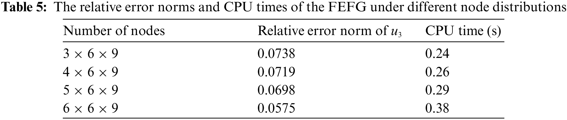
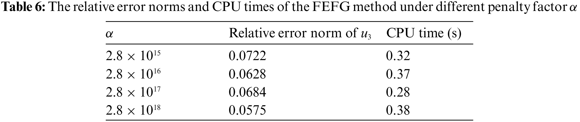
Table 6 illustrates the calculation accuracies and CPU running times of the FEFG method when the penalty factor is different. For this case, we choose for the FEFG method.

Figs. 14–16 show the calculation outcomes of the FEFG method, the IEFG method and the analytical results of displacement and the distribution of the normal stresses and along direction , respectively. It can be seen that the results of the FEFG method are closer to the analytical solution than those of the IEFG method.

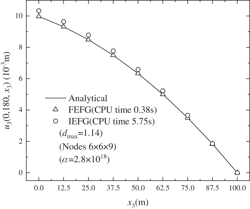
Figure 14: The distribution of the displacement along

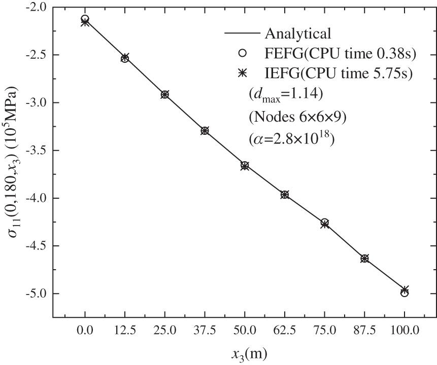
Figure 15: The distribution of the normal stress along

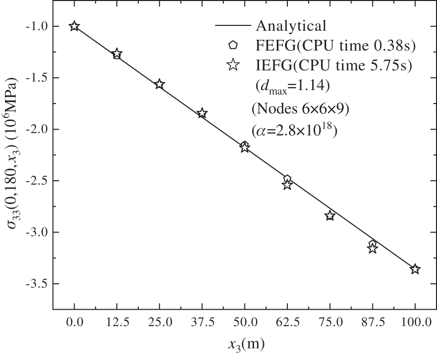
Figure 16: The distribution of the normal stress along

4.4 Hollow Cylinder Subjected to Internal Pressure

Consider a hollow cylinder subjected to uniform internal pressure. Fig. 17 shows the quarter region and Fig. 18 shows the nodes arrangement on the quarter model on each plane . The inner surface is subjected to uniformly distributed pressure , Poisson's radio is , the Young's modulus is . The inner and outer radius of the cylinder are and , respectively, and the height of the cylinder . The analytical solution of the problem is

(104)

(105)

(106)

(107)

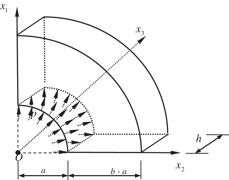
Figure 17: A hollow cylinder under distributed internal pressure

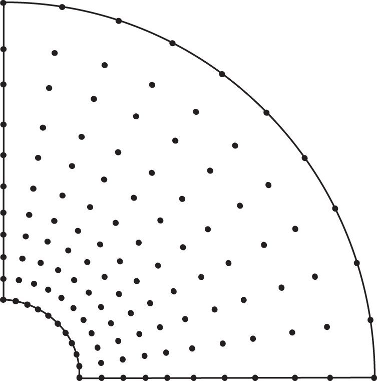
Figure 18: Nodes arrangement on the quarter model on each plane

We only consider a quarter of the problem domain. Selecting the IEFG method to solve this problem, 11 × 11 × 5 nodes are selected. and . Then, the CPU running time is 22.71 s, and the overall relative error norm of is .

Next, the FEFG method is selected to solve this problem. The direction is the splitting direction. Three planes are inserted along direction . On plane , 11 × 11 nodes are distributed as shown in Fig. 18. In addition, and . Then, the CPU running time is 1.47 s, and the overall relative error norm of is similar to that of the IEFG method. It can be seen that the FEFG method is much faster than the IEFG method in solving the solution of this case.

Figs. 19–21 show the calculation outcomes of the FEFG method, the IEFG method and the analytical results of displacement , stress and along direction r, respectively. It can be found that the numerical results obtained by the FEFG method and the IEFG method are in good agreement with the analytical solutions, and the FEFG method runs faster than the IEFG method.

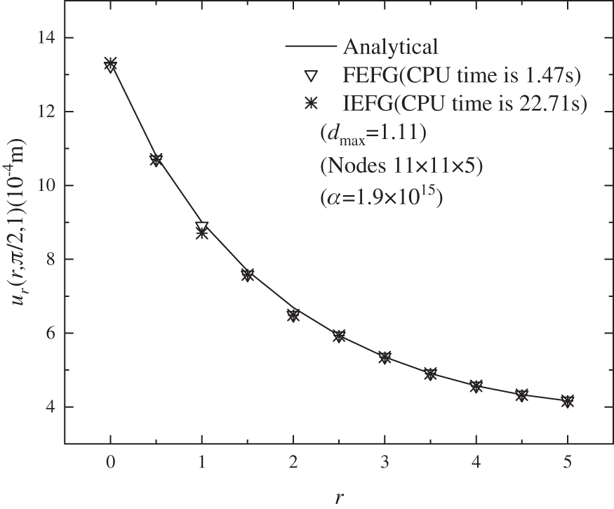
Figure 19: The distribution of the normal displacement along

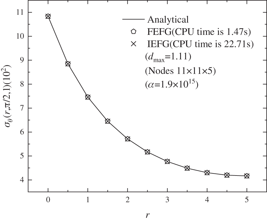
Figure 20: The distribution of the normal stress along

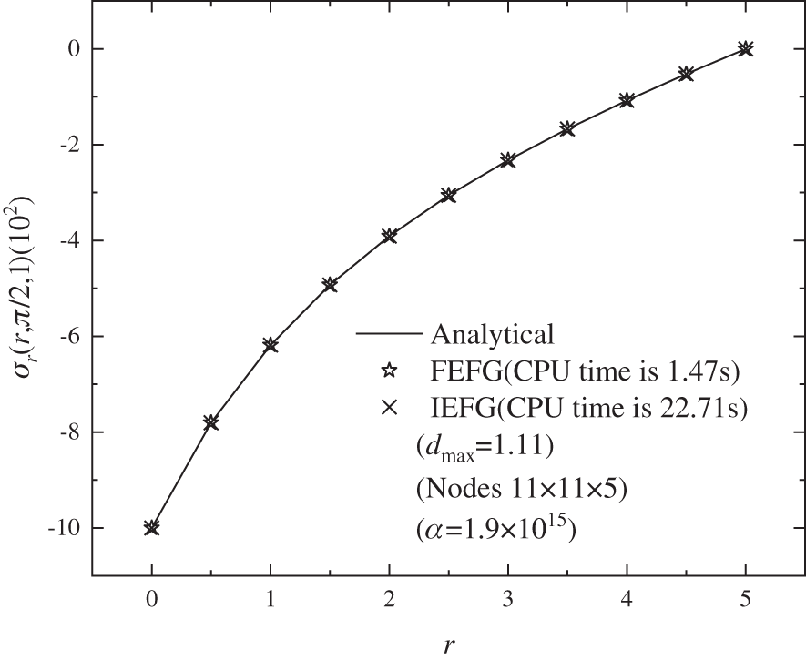
Figure 21: The distribution of the normal stress along

5  Conclusions

In this paper, the FEFG method for the 3D elasticity problem is established. The 3D elasticity problems are divided into a set of related 2D problems along the dimension splitting direction. Then, the IEFG method is chosen to solve these 2D problems. The FDM is selected in the dimension splitting direction. The final solvable discrete system equations of the 3D elasticity problem are obtained. In contrast to the IEFG method, the FEFG method saves the computing time of the shape function by reducing the dimensionality. Furthermore, the numerical results of the FEFG method and the IEFG method are both agree with the analytical results. Numerical examples indicate that the FEFG method for three-dimensional elasticity problems is efficient and convergent.

Funding Statement: This work was supported by the National Natural Science Foundation of China (Grant Nos. 52004169 and 11571223).

Conflicts of Interest: The authors declare that they have no conflicts of interest to report regarding the present study.

References

 1.  Hoang, T. T. P., Vo, D. C. H., Ong, T. H. (2017). A Low-order finite element method for three dimensional linear elasticity problems with general meshes. Computers & Mathematics with Applications, 74(6), 1379–1398. DOI 10.1016/j.camwa.2017.06.023. [Google Scholar] [CrossRef]

 2.  Hossain, M. Z., Ahmed, S. R., Uddin, M. W. (2005). A new mathematical model for finite-difference solution of three-dimensional mixed-boundary-value elastic problems. International Journal of Computational Methods, 2(1), 99–126. DOI 10.1142/S0219876205000387. [Google Scholar] [CrossRef]

 3.  Popov, V., Power, H. (2001). An O(N) Taylor series multipole boundary element method for three-dimensional elasticity problems. Engineering Analysis with Boundary Elements, 25(1), 7–18. DOI 10.1016/S0955-7997(00)00052-7. [Google Scholar] [CrossRef]

 4.  Zhang, Z., Liew, K. M. (2010). Improved element-free Galerkin method (IEFG) for solving three-dimensional elasticity problems. Interaction & Multiscale Mechanics, 3(2), 123–143. DOI 10.1016/S0955-7997(00)00052-7. [Google Scholar] [CrossRef]

 5.  Miao, Y., Wang, Y. H. (2006). Meshless analysis for three-dimensional elasticity with singular hybrid boundary node method. Applied Mathematics & Mechanics, 27(5), 673–681. DOI 10.1007/s10483-006-0514-z. [Google Scholar] [CrossRef]

 6.  Li, X. L. (2012). A priori and a posteriori analysis of the meshless Galerkin boundary node method for three-dimensional elasticity. Engineering Analysis with Boundary Elements, 36, 993–1004. DOI 10.1016/j.enganabound.2011.12.015. [Google Scholar] [CrossRef]

 7.  Alavi, S. M. R., Aghdam, M. M., Eftekhari, A. (2006). Three-dimensional elasticity analysis of thick rectangular laminated composite plates using meshless local Petrov-Galerkin (MLPG) method. Applied Mechanics & Materials, 5–6, 331–338. DOI 10.4028/www.scientific.net/AMM.5-6.331. [Google Scholar] [CrossRef]

 8.  Cheng, Y. M., Chen, M. J. (2003). A boundary element-free method for linear elasticity. Acta Mechanica Sinica, 35(2), 435–448. DOI 10.3321/j.issn:0459-1879.2003.02.010. [Google Scholar] [CrossRef]

 9.  Dai, B. D., Cheng, Y. M. (2007). Local boundary integral equation method based on radial basis functions for potential problems. Acta Physica Sinica, 56(2), 597–603. DOI 10.7498/aps.56.597. [Google Scholar] [CrossRef]

10. Bai, F. N., Li, D. M., Wang, J. F. (2012). An improved complex variable element-free Galerkin method for two-dimensional elasticity problems. Chinese Physics B, 21(2), 020204. DOI 10.1088/1674-1056/21/2/020204. [Google Scholar] [CrossRef]

11. Cheng, Y. M., Liu, C., Bai, F. N. (2015). Analysis of elastoplasticity problems using an improved complex variable element-free Galerkin method. Chinese Physics B, 24(10), 16–25. DOI 10.1088/1674-1056/24/10/100202. [Google Scholar] [CrossRef]

12. Abbaszadeh, M., Khodadadian, A., Parvizi, M., Dehghan, M., Heitzinger, C. (2018). A direct meshless local collocation method for solving stochastic cahn–hilliard–cook and stochastic swift–hohenberg equations. Engineering Analysis with Boundary Elements, 98, 253–264. DOI 10.1016/j.enganabound.2018.10.021. [Google Scholar] [CrossRef]

13. Wu, Q., Peng, P. P., Cheng, Y. M. (2021). The interpolating element-free Galerkin method for elastic large deformation problems. Science China Technological Sciences, 64, 364–374. DOI 10.1007/s11431-019-1583-y. [Google Scholar] [CrossRef]

14. Cheng, J. (2020). Data analysis of the factors influencing the industrial land leasing in shanghai based on mathematical models. Mathematical Problems in Engineering, 2020, 1–11. DOI 10.1155/2020/9346863. [Google Scholar] [CrossRef]

15. Cheng, J. (2021). Mathematical models and data analysis of residential land leasing behavior of district governments of Beijing in China. Mathematics, 9, 2314. DOI 10.3390/math9182314. [Google Scholar] [CrossRef]

16. Cheng, J. (2020). Analyzing the factors influencing the choice of the government on leasing different types of land uses: Evidence from shanghai of China. Land Use Policy, 90, 104303. DOI 10.1016/j.landusepol.2019.104303. [Google Scholar] [CrossRef]

17. Cheng, J. (2021). Residential land leasing and price under public land ownership. Journal of Urban Planning and Development, 147(2), 5021009. DOI 10.1061/(ASCE)UP.1943-5444.0000701. [Google Scholar] [CrossRef]

18. Cheng, J. (2021). Analysis of commercial land leasing of the district governments of Beijing in China. Land Use Policy, 100, 104881. DOI 10.1016/j.landusepol.2020.104881. [Google Scholar] [CrossRef]

19. Zhang, Z., Wang, J. F., Cheng, Y. M., Liew, K. M. (2013). The improved element-free Galerkin method for three-dimensional transient heat conduction problems. Science China, 8(2), 153–165. DOI 10.1007/s11433-013-5135-0. [Google Scholar] [CrossRef]

20. Zhang, Z., Zhao, P., Liew, K. M. (2009). Analyzing three-dimensional potential problems with the improved element-free Galerkin method. Acta Mechanica Sinica, 44(2), 273–284. DOI 10.1007/s00466-009-0364-9. [Google Scholar] [CrossRef]

21. Zhang, Z., Li, D. M., Cheng, Y. M., Liew, K. M. (2012). The improved element-free Galerkin method for three-dimensional wave equation. Acta Mechanica Sinica, 28(3), 808–818. DOI 10.1007/s10409-012-0083-x. [Google Scholar] [CrossRef]

22. Abbaszadeh, M., Dehghan, M., Khodadadian, A., Heitzinger, M. (2019). Analysis and application of the interpolating element free Galerkin (IEFG) method to simulate the prevention of groundwater contamination with application in fluid flow. Journal of Computational and Applied Mathematics, 112453. DOI 10.1016/j.cam.2019.112453. [Google Scholar] [CrossRef]

23. Peng, M. J., Li, R. X., Cheng, Y. M. (2014). Analyzing three-dimensional viscoelasticity problems via the improved element-free Galerkin (IEFG) method. Engineering Analysis with Boundary Elements, 40, 104–113. DOI 10.1016/j.enganabound.2013.11.018. [Google Scholar] [CrossRef]

24. Zheng, G. D., Cheng, Y. M. (2020). The improved element-free Galerkin method for diffusional drug release problems. International Journal of Applied Mechanics and Engineering, 12(8), 2050096. DOI 10.1142/S1758825120500969. [Google Scholar] [CrossRef]

25. Yu, S. Y., Peng, M. J., Cheng, H., Cheng, Y. M. (2019). The improved element-free Galerkin method for three-dimensional elastoplasticity problems. Engineering Analysis with Boundary Elements, 104, 215–224. DOI 10.1016/j.enganabound.2019.03.040. [Google Scholar] [CrossRef]

26. Liu, F. B., Cheng, Y. M. (2018). The improved element-free Galerkin method based on the nonsingular weight functions for elastic large deformation problems. International Journal of Applied Mechanics, 7, 1850023. DOI 10.1142/S2047684118500239. [Google Scholar] [CrossRef]

27. Liu, F. B., Cheng, Y. M. (2018). The improved element-free Galerkin method based on the nonsingular weight functions for inhomogeneous swelling of polymer gels. International Journal of Applied Mechanics, 10, 1850047. DOI 10.1142/S1758825118500473. [Google Scholar] [CrossRef]

28. Cai, X. J., Peng, M. J., Cheng, Y. M. (2018). The improved element-free Galerkin method for elastoplasticity large deformation problems. Scientia Sinica-Physica,Mechanica & Astronomica, 48, 24701. DOI 10.1360/SSPMA2017-00231. [Google Scholar] [CrossRef]

29. Wu, Y., Ma, Y. Q., Feng, W., Cheng, Y. M. (2017). Topology optimization using the improved element-free Galerkin method for elasticity. Chinese Physics B, 26, 80203. DOI 10.1088/1674-1056/26/8/080203. [Google Scholar] [CrossRef]

30. Zou, S. Y., Xi, W. C., Peng, M. J., Cheng, Y. M. (2017). Analysis of fracture problems of airport pavement by improved element-free Galerkin method. Acta Physica Sinica, 66, 120204. DOI 10.7498/aps.66.120204. [Google Scholar] [CrossRef]

31. Cheng, R. J., Cheng, Y. M. (2016). Solving unsteady schrödinger equation using the improved element-free Galerkin method. Chinese Physics B, 25, 020203-1-9. DOI 10.1088/1674-1056/25/2/020203. [Google Scholar] [CrossRef]

32. Cheng, Y. M., Bai, F. N., Liu, C., Peng, M. J. (2016). Analyzing nonlinear large deformation with an improved element-free Galerkin method via the interpolating moving least-squares method. International Journal of Applied Mechanics and Engineering, 5, 1650023-1-22. DOI 10.1142/S2047684116500238. [Google Scholar] [CrossRef]

33. Li, K. T., Shen, X. Q. (2007). A dimensional splitting method for the linearly elastic shell. International Journal of Computational Mechanics, 84, 807–824. DOI 10.1080/00207160701458328. [Google Scholar] [CrossRef]

34. Chen, H., Li, K. T., Wang, S. (2013). A dimension split method for the incompressible Navier–Stokes equations in three dimensions. International Journal for Numerical Methods in Fluids, 73, 409–435. DOI 10.1002/fld.3803. [Google Scholar] [CrossRef]

35. Hou, Y. R., Wei, H. B. (2012). Dimension splitting algorithm for a three-dimensional elliptic equation. International Journal of Computational Mechanics, 89, 112–127. DOI 10.1080/00207160.2011.631531. [Google Scholar] [CrossRef]

36. ter Maten, E. J. W. (1986). Splitting methods for fourth order parabolic partial differential equations. Computing, 37, 335–350. DOI 10.1007/BF02251091. [Google Scholar] [CrossRef]

37. Bragin, M. D., Rogov, B. V. (2016). On exact dimensional splitting for a multidimensional scalar quasilinear hyperbolic conservation law. Doklady Mathematics, 94, 382–386. DOI 10.1134/S1064562416040086. [Google Scholar] [CrossRef]

38. Meng, Z. J., Cheng, H., Ma, L. D., Cheng, Y. M. (2018). The dimension split element-free Galerkin method for three-dimensional potential problems. Acta Mechanica Sinica, 34, 50–62. DOI 10.1007/s10409-017-0747-7. [Google Scholar] [CrossRef]

39. Meng, Z. J., Cheng, H., Ma, L. D., Cheng, Y. M. (2019). The hybrid element-free Galerkin method for three-dimensional wave propagation problems. International Journal for Numerical Methods in Engineering, 117, 15–37. DOI 10.1002/nme.5944. [Google Scholar] [CrossRef]

40. Ma, L. D., Meng, Z. J., Chai, J. F., Cheng, Y. M. (2020). Analyzing 3D advection-diffusion problems by using the dimension splitting element-free Galerkin method. Engineering Analysis with Boundary Elements, 111, 167–177. DOI 10.1016/j.enganabound.2019.11.005. [Google Scholar] [CrossRef]

41. Meng, Z. J., Cheng, H., Ma, L. D., Cheng, Y. M. (2019). The dimension splitting element-free Galerkin method for 3D transient heat conduction problems. Science China, 62, 040711. DOI 10.1007/s11433-018-9299-8. [Google Scholar] [CrossRef]

42. Cheng, H., Peng, M. J., Cheng, Y. M. (2017). The hybrid improved complex variable element-free Galerkin method for three-dimensional potential problems. Engineering Analysis with Boundary Elements, 84, 52–62. DOI 10.1016/j.enganabound.2017.08.001. [Google Scholar] [CrossRef]

43. Cheng, H., Peng, M. J., Cheng, Y. M. (2018). The dimension splitting and improved complex variable element-free Galerkin method for 3-dimensional transient heat conduction problems. International Journal of Applied Mechanics, 114, 321–345. DOI 10.1002/nme.5745. [Google Scholar] [CrossRef]

44. Cheng, H., Peng, M. J., Cheng, Y. M. (2017). A fast complex variable element-free Galerkin method for three-dimensional wave propagation problems. International Journal of Applied Mechanics, 9, 1750090. DOI 10.1142/S1758825117500909. [Google Scholar] [CrossRef]

45. Cheng, H., Peng, M. J., Cheng, Y. M. (2020). The hybrid complex variable element-free Galerkin method for 3D elasticity problems. Engineering Structures, 219, 110835. DOI 10.1016/j.engstruct.2020.110835. [Google Scholar] [CrossRef]

46. Wu, Q., Peng, M. J., Fu, Y. D., Cheng, Y. M. (2021). The dimension splitting interpolating element-free Galerkin method for solving three-dimensional transient heat conduction problems. Engineering Analysis with Boundary Elements, 128, 326–341. DOI 10.1016/j.enganabound.2021.04.016. [Google Scholar] [CrossRef]

47. Wu, Q., Peng, M. J., Cheng, Y. M. (2021). The interpolating dimension splitting element-free Galerkin method for 3D potential problems. Engineering with Computers, 1–4. DOI 10.1007/s00366-021-01408-5. [Google Scholar] [CrossRef]

48. Liu, W. K., Jun, S., Li, S., Adee, J., Belytschko, T. (1995). Reproducing kernel particle methods for structural dynamics. International Journal for Numerical Methods in Engineering, 38, 1655–1679. DOI 10.1002/nme.1620381005. [Google Scholar] [CrossRef]

49. Liu, W. K., Li, S., Belytschko, T. (1997). Moving least square reproducing kernel method (I) Methodology and convergence. Computer Methods in Applied Mechanics and Engineering, 143(1–2), 113–154. DOI https://dx.doi.org/10.1016/S0045-7825(96)01132-2. [Google Scholar]

50. Li, S. F., Liu, W. K. (1999). Reproducing kernel hierarchical partition of unity, part I: Formulations. International Journal for Numerical Methods in Engineering, 45, 251–288. DOI 10.1002/(SICI)1097-0207(19990530)45:3<251::AID-NME583>3.0.CO;2-I. [Google Scholar] [CrossRef]

51. Peng, P. P., Cheng, Y. M. (2021). Analyzing three-dimensional wave propagation with the hybrid reproducing kernel particle method based on the dimension splitting method. Engineering with Computers, 3, 1–17. DOI 10.1007/S00366-020-01256-9. [Google Scholar] [CrossRef]

52. Peng, P. P., Cheng, Y. M. (2020). Analyzing three-dimensional transient heat conduction problems with the dimension splitting reproducing kernel particle method. Engineering Analysis with Boundary Elements, 121, 180–191. DOI 10.1016/j.enganabound.2020.09.011. [Google Scholar] [CrossRef]

53. Peng, P. P., Wu, Q., Cheng, Y. M. (2020). The dimension splitting reproducing kernel particle method for three-dimensional potential problems. International Journal for Numerical Methods in Engineering, 121, 146–164. DOI 10.1002/nme.6203. [Google Scholar] [CrossRef]

54. Yang, J. J., Wen, P. H. (2018). Meshless method theories and approaches. Beijing: Science press. [Google Scholar]

This work is licensed under a Creative Commons Attribution 4.0 International License, which permits unrestricted use, distribution, and reproduction in any medium, provided the original work is properly cited.