Computer Modeling in Engineering & Sciences

DOI: 10.32604/cmes.2022.019970

ARTICLE

An Optimized Convolutional Neural Network with Combination Blocks for Chinese Sign Language Identification

Yalan Gao, Yanqiong Zhang and Xianwei Jiang*

Nanjing Normal University of Special Education, Nanjing, 210038, China
*Corresponding Author: Xianwei Jiang. Email: jxw@njts.edu.cn
Received: 29 October 2021; Accepted: 15 December 2021

1  Introduction

According to statistics, there are hundreds of millions of deaf people in the world, and there are more than 27.9 million deaf people in China [1]. As a visual language, sign language plays an important role in the life of most deaf people. It is an essential tool for them to live, learn and communicate in deaf communities all over the word. Sign language, like vocal language, is naturally produced and expresses information according to its own grammatical rules [2]. Experts in sign language use the term “phonology” to refer to the study of the structure and composition of gestures. Signs in sign language have five basic components: hand shape, movement, position, direction and non-manual features [3]. However, fewer people can understand sign language because of its complexity. This leads to a real communication barrier between the deaf community and the rest of society. At present, two solutions are being tried to solve the problem. One method is to convert speech into text for the deaf to see, namely, intelligent speech recognition, such as seeing of iFLYTEK. Another method is to convert sign language into text or speech, namely sign language recognition, which is what we want to discuss.

Sign Language Recognition (SLR) automatically converts sign language into text, speech and so on by computer technology, which involves computer vision, pattern recognition, human-computer interaction, etc. It has important research significance and application value. Some early efforts on SLR can be dated back to the 1990s. According to the different acquisition methods of sign language data, there are two main categories of the SLR system: sensor-based and vision-based. The former needs to use devices equipped with sensors to extract the shape and motion of gestures, the latter obtains images and videos from the camera [4]. From the research object, sign language recognition can be divided into finger spelling recognition, isolated word recognition and continuous sentence recognition.

Among traditional machine learning models, Hidden Markov Models (HMM) are widely employed in sign language recognition, and literature [5–7] have introduced them. In addition, Support Vector Machines (SVM) are also the most commonly adopted method for sign language recognition. Literature [8–11] all mentioned the content of sign language recognition by support vector machine alone or in combination. Traditional manual feature extraction and classification are two important components of traditional machine learning models, in literature [12–14], some classical algorithms of images processing and recognition were discussed diffusely. In recent years, modern convolutional neural networks have been diffusely applied in the field of image recognition [15,16]. Vision-based sign language image recognition occupies a large proportion of sign language recognition. Literature [17–22] have a different description of this. The deep neural network owns the ability of self-learning and self-organization, with the power of computing enhancing, it can achieve better performance. Furthermore, some other design methods are mentioned in researches [23–29]. Dynamic Time Warping (DTW), Long Short-Term Memory (LSTM) [30], BLSTM-3D ResNet [31], k-nearest neighbor (k-NN), skin color modeling, random forest, extreme learning machine (ELM) and key-frame-based center editing method are all very classic and effective. Although many different algorithms and approaches were proposed, they all have some limitations and application scenarios. Thus, it is not easy to give the comparisons and evaluations scientifically.

In this paper, an optimized convolutional neural network with combination blocks (CNN-CB) for Chinese Sign language identification was proposed. Different combinations of blocks were tried. This convolutional neural network is fully optimized on each block. Besides, advanced technologies of batch normalization, dropout, and Leaky ReLU were introduced to achieve excellent performance. In the experiments, we compared pooling methods, activation functions, dropout rate and different permutations of combination blocks, respectively. Finally, we compared the proposed method with the 13 state-of-the-art methods, and the results show that our method is superior.

2  Dataset

Although Chinese sign language is divided into gesture sign language and fingerspelling sign language, fingerspelling sign language is the most certain, which can be used as the element of Pinyin words. On the contrary, gesture sign language has local differences and is not unique. Therefore, images of Chinese fingerspelling sign language are employed in our data set, including a total of 1320 images and 30 categories. Here, thirty categories include the letters a to z, and the two-syllable letters zh, ch, sh, and ng. Meanwhile, each category has 44 images from volunteers. Every image was preprocessed with size of 256 × 256. As shown in Fig. 1, a sample that contains all categories is demonstrated. Besides, to help understand and focus on the abbreviated words, a list of abbreviations is shown in Table 1.

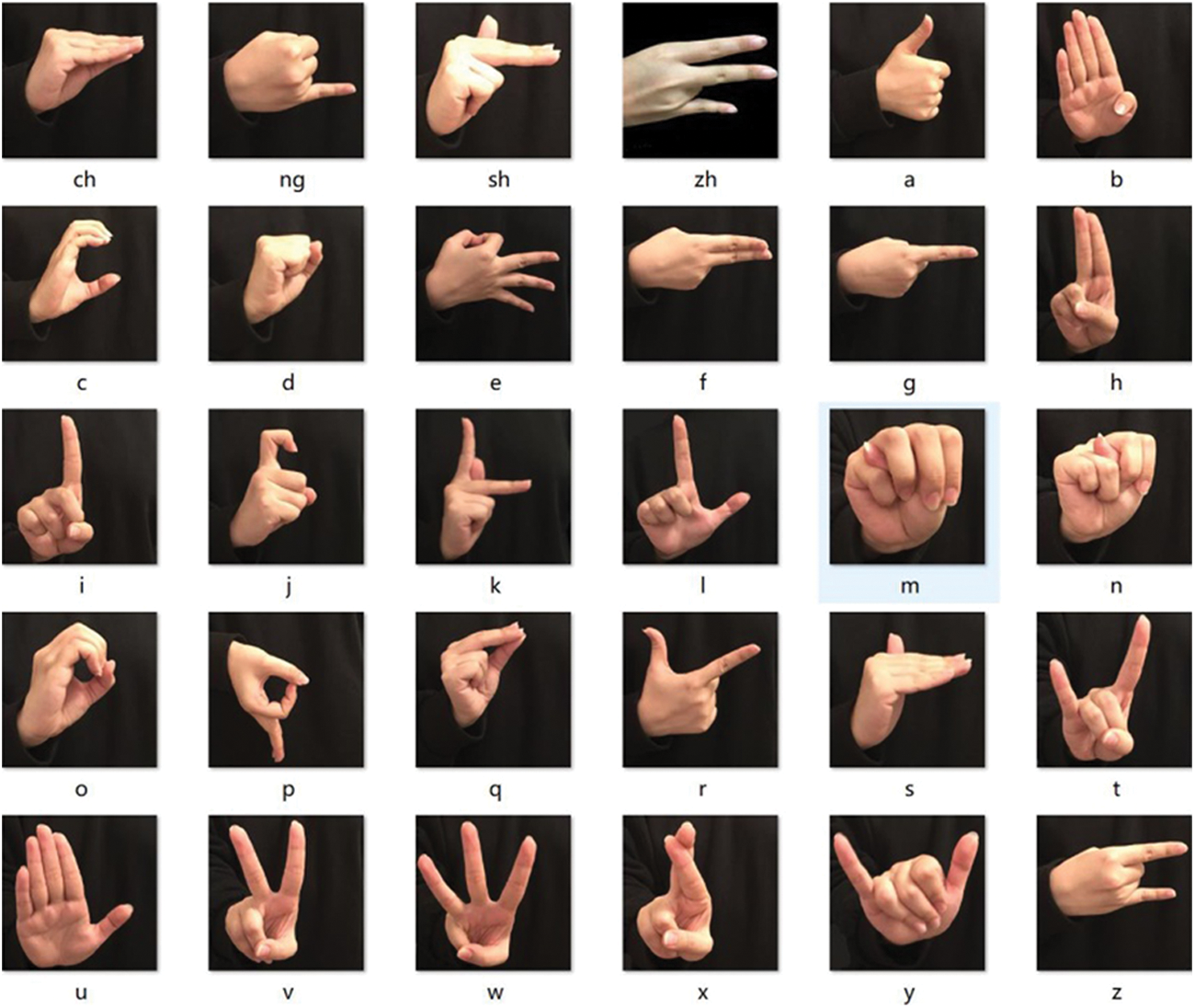
Figure 1: A sample of Chinese sign language

3  Methodology

3.1 Convolutional Layer

Many neurons have been found to have a small local receptive field in the visual cortex, responding only to visual stimuli within a limited area of the visual field. The receptive fields of different neurons overlap to form a complete field of vision. Different neurons respond to different parts of the field, like lines at different angles, and different neurons in the same receiving field respond to different parts of the field. Some neurons have a larger receptive field and respond to complex patterns made up of low-level patterns. This structure enables the visual cortex to detect all the complex and simple patterns in the field of vision. The above research results contributed to the emergence of neurocognitive machines, which eventually developed into convolutional neural networks (CNN) [32].

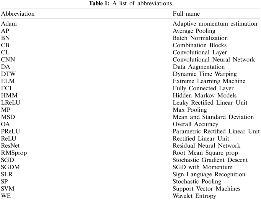
The convolutional layer (CL) is the most important part of convolutional neural network [33]. More convolutional layers are used to obtain deeper feature information. After many convolutions, features in the image can be extracted. Through a simple instance, Fig. 2 illustrates the process of convolution operation: input a 4 × 4 image, after two 2 × 2 convolution kernels carry out convolution operation, it becomes a 3 × 3 feature image. The convolution layer slides over the input layer with a step of 1.

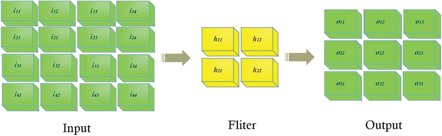
Figure 2: The process of convolution operation

Compute the input of the first convolutional layer nerve o11:

conv(input,fliter)=i11×h11+i12×h12+i21×h21+i22×h22

The calculation method of the neurons is the same. After all the outputs are calculated, the whole output graph is obtained. Generally, we use more convolutional layers to obtain deeper feature information.

The convolutional layer has such feature as “incomplete connection and parameter sharing”, which greatly reduces network parameters, ensures network sparsity and prevents over-fitting.

3.2 Pooling Layer

Adjacent pixels in the image tend to have similar values, so usually adjacent output pixels in the convolution layer also have similar values. This means that most of the information contained in the output of the convolution layer is redudent. Therefore, it is believed that image features can be represented at a higher level of abstraction. The pooling layer solves this problem. The role of the pooling layer is to reduce the number of output values by reducing the size of the input or reducing the dimensionality.

Pooling layer is usually sandwiched between continuous convolutional layers, which is used to compress the amount of the parameters, reduce over-fitting and improve robustness. Its specific operation is basically the same as that of the convolutional layer, except that the convolution kernel of the pooling layer only takes the maximum or average value of the corresponding position [34]. Therefore, the pooling layer can also be divided into Max Pooling (MP), Average Pooling (AP) and Stochastic Pooling (SP), etc. [35–37]. Max Pooling and Average Pooling are widely used. Because the size of the convolution kernel can be reduced through pooling and the corresponding features can be retained, it is mainly used for dimensionality reduction [38,39].

Pooling is typically carried out through relatively simple maximum, minimum, or average operations. As shown in Figs. 3 and 4, an example of max pooling with a pool size of 2 and an average pooling sample with the same parameters are given as follows.

Figure 3: An example of max pooling

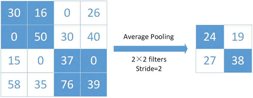
Figure 4: An example of average pooling

Average pooling is realized by averaging the values in the field, which can restrain the variance increase of estimated values due to the limitation of neighborhood size, and is characterized by better background retention effect. Max pooling is achieved by taking the maximum value of feature in the neighborhood, which can suppress the phenomenon of estimated mean caused by network parameter errors and better extract texture information. In this paper, we compared the two methods to extract feature information.

Additionally, in stochastic pooling, the elements in the feature map are randomly selected based on their probability values. Stochastic pooling ensures that neurons with non-maximum response values in the feature map can enter the next layer for extraction. Thus, it makes stochastic pooling have stronger generalization ability and avoid over-fitting. As shown in Fig. 5, an example of SP was provided, which demonstrated the whole process from the original map to generating a probability map and finally gaining stochastic pooling output.

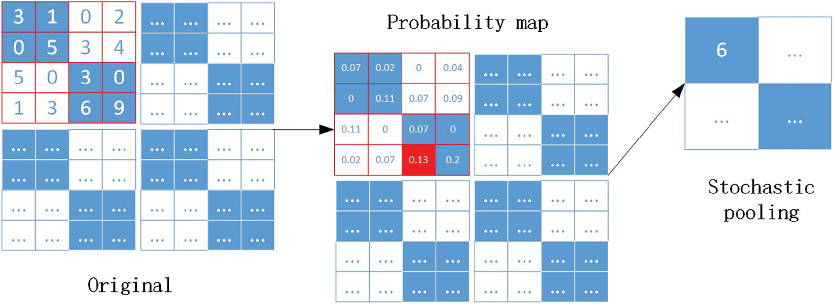
Figure 5: An example of stochastic pooling

3.3 Batch Normalization

In the process of deep network training, internal covariate shift changes data distribution of internal nodes due to changes in network parameters [40]. This requires the upper-layer network to constantly adjust to the change of input data distribution, but will lead to the decrease of network learning speed, network training process is prone to fall into gradient saturation zone, slowing down the network convergence speed [41]. Batch normalization (BN) can solve this problem by smoothing and optimizing the solution space, regularization is achieved.

The BN approach, which greatly accelerates models training while maintaining predictive accuracy, has been adopted as a standard model layer by some good models. The training of deep neural networks often requires repeated initialization of debugging parameters, and the utilization of small learning rate parameters results in slow training. In addition, the saturated nonlinear model, the function derivative tends to 0 in the saturated region, also makes the model difficult to train. Before the nonlinear layer, the BN method stabilizes the input distribution of each layer by controlling the mean and variance of input distribution of each layer, thus promoting the training effect.

The BN is a step that converts the input of mini-batch into approximate normal distribution by using standardized variables. Take a mini-batch with a capacity of N as sample set X, and calculate each single example in turn.

μbatch=1n∑i=1n⁡xi(1)

σ2batch=1n∑i=1n⁡(xi−μbatch)2(2)

xi^=xi−μbatchσ2batch+δ(3)

yi=αxi^+γ(4)

The denominator of Eq. (3) δ is a smoothing term, which is used to avoid zero-error in the case of minimal variance. Observe the first three steps, normalize the input data into standardized variables with mean 0 and variance approximately 1, and then perform scaling and shifting through linear transformation of Eq. (4). Learn the appropriate scale of scaling and translation through the parameter training of α and γ to restore model expression, then get the batch norm output of mini-batch. After the training, the parameter α and γ are learned.

The expectation after transformation is:

M(xi^)=1σ2batch+δM(x−μbatch)=1σ2batch+δ[M(x)−μbatch]=0(5)

The variance after transformation is:

Var(xi^)= M{[xi^−M(xi^)]2}=M{xi^2−2xi^M(xi^)+[M(xi^)]2}              =M(xi^2)−2[M(xi^)]2+[M(xi^)]2=M(xi^2)−[M(xi^)]2              =M[(x−μbatchσ2batch+δ )2]=1σ2batch+δM[(x−μbatch)2]              =μbatch2μbatch2+δ≈1  (6)

Due to the small value of the smoothing factor δ, the mean value of the transformed result is 0 and the variance is close to 1.

The two learnable parameters α and  γ was introduced in BN. The introduction of these two parameters is to restore the expression ability of the data itself and perform linear transformation on normalized data. In particular, when α2=σ2 and  γ=μ, can achieve identity transformation and retain the distribution information of the original input features.

According to the results, the neural network generally uses BN to achieve better training effect and has the following advantages: i) It allows the network to use saturation activation function, alleviates the gradient transfer problem; ii) It makes the input data of each layer in the network relatively stable, and accelerates the speed of model learning; iii) It makes the model less sensitive to the parameters in the network, simplifies the parameter turning process, and makes the network learning more stable. iv) It has a certain regularization effect.

3.4 ReLU, Leaky ReLU and Parametric ReLU

3.4.1 ReLU

Activation function is a function added to an artificial neural network to help the network learn complex patterns in data. Similar to the neuron-based model in the human brain, the activation function ultimately determines what to fire into the next neuron.

Rectified linear unit (ReLU) function is a popular activation function in deep learning [42–44]. The illustration of ReLU activation function is shown in Fig. 6.

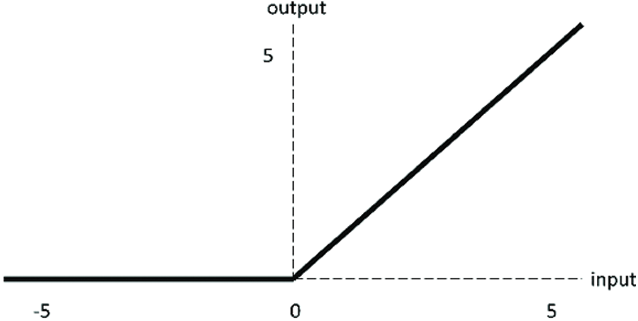
Figure 6: The illustration of ReLU activation function

The corresponding function expression is:

σy={max(0,y),y≥00,y<0(7)

ReLU itself is a piecewise linear function, but it can continuously approach a nonlinear function piecewise. Compared with general Sigmoid function and TANH function, ReLU function has the following advantages: i) ReLU has sparsity, which enables the sparse model to better mine relevant features and fit training data; ii) Calculations are much faster. ReLU function has only linear relationships, so it can be computed faster than Sigmoid and TANH; iii) In the region y > 0, the problem of gradient saturation and gradient disappearance does not occur; iv) Low computational complexity, no exponential operation is required, as long as a threshold value can be obtained.

3.4.2 Leaky ReLU

In the ReLU function, if the input to the activation function is negative for all sample inputs, then the neuron can no longer learn, which is called Dead ReLU problem. Leaky rectified linear unit (LReLU) is an activation function specifically designed to solve the Dead ReLU problem.

Leaky ReLU is very similar to ReLU, with the difference only in the part of the input less than 0 where the value of ReLU is 0, while the part of the input less than 0 is negative and has a slight gradient [45]. Fig. 7 shows the function image of Leaky ReLU.

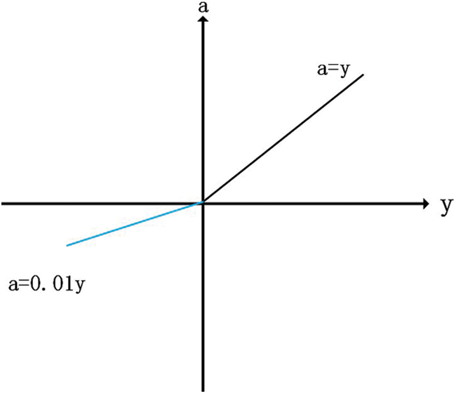
Figure 7: The illustration of Leaky ReLU

The corresponding function expression is:

f(yi)={yi,yi>0ayi,yi≤0(aisusually0.01)(8)

In addition to all the advantages inherited from ReLU, Leaky ReLU has the following advantages: i) Leaky ReLU adjusts the negative zero gradient problem by giving a very small linear component of y to a negative input of 0.01y; ii) Leak helps to expand the scope of ReLU function, usually a value is about 0.01; iii) Leaky ReLU's function range is negative infinity to positive infinity. But the result of this function is not consistent. Although it has all the characteristic of ReLU activation functions, such as computational efficiency, fast convergence, and no saturation in the positive region.

3.4.3 Parametric ReLU (PReLU)

In LReLU, a is a fixed constant. Parametric ReLU (PReLU) proposed to learn the optimal value of δ from the data propagation itself through back propagation [46,47]. This provides a more general rectifier function where the additional computational cost is negligible. By sharing δ across channels, the number of additional learnable parameters is further reduced (see Fig. 8)

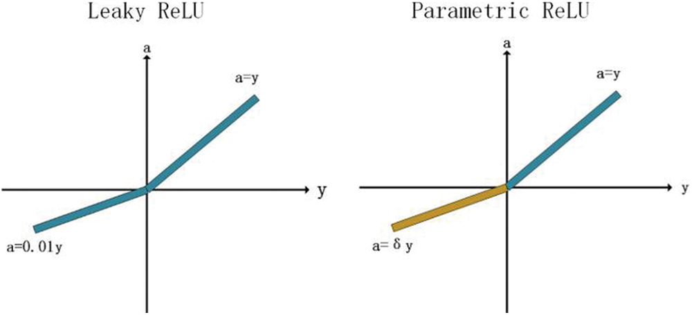
Figure 8: Comparison of Leaky ReLU and Parametric ReLU

Parameter δ is usually a number between 0 and 1, and is usually relatively small.

3.5 Dropout

Since large-scale neural networks are time-consuming and prone to overfitting, the advent of dropout solves both problems. Dropout came to the fore in 2012, when Hinton wrote about dropout in a paper. When a complex feedforward neural network is trained on a small dataset, it is easy to overfit. In order to prevent overfitting, the performance of neural network can be improved by preventing the interaction of feature detectors [48].

Dropout typically applies to the output of the full connection layer (FCL) [49]. If there is over-fitting for the neural network, the neural network discards neurons randomly in a certain proportion through the dropout layer, so that the network model in each training will be different. Multiple epochs are equivalent to training multiple models, and each model participated in the vote on the final result, this not only reduces the scale of the neural network, but also prevents over-fitting and improves the generalization ability of the model [50,51].

In the training process of each iteration, we randomly throw away part of the neurons. In view of the network nodes in each layer is set to eliminate neural network of probability, the frame for the dotted neurons are discarded, and then deleted from the node in and out of attachment, finally get a node less, smaller networks, then the network structure in this training will be simplifies. The schematic diagram of dropout was shown in Fig. 9.

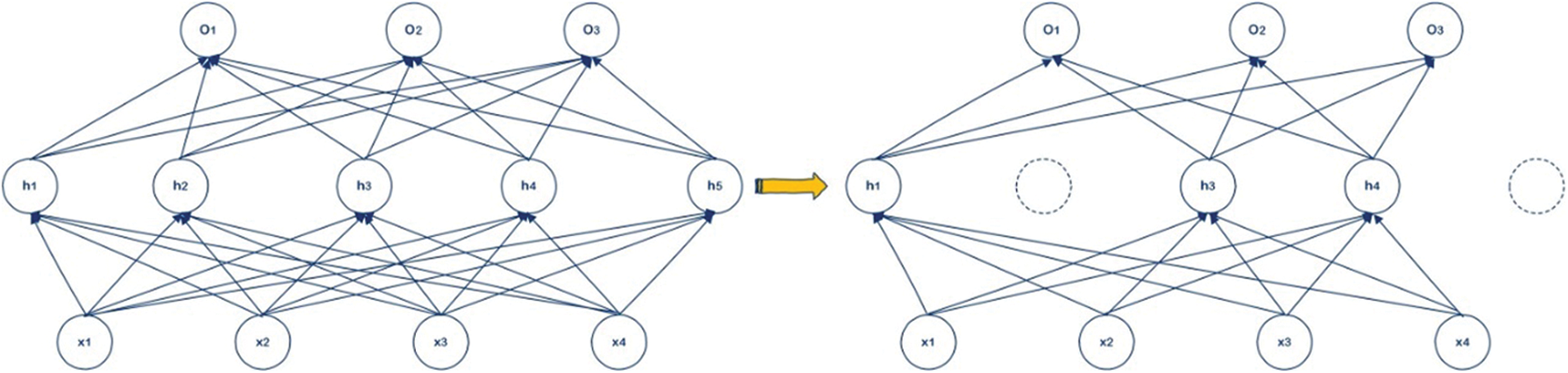
Figure 9: Schematic diagram of dropout

In addition, according to the traditional dropout theory, it should discard several pixels on the feature map. However, this approach is not very effective in CNN, and an important reason is the similarity between adjacent pixels. Because not only are they very close in terms of the input values, but they have similar neighbors, similar receptive fields, and the same convolution kernel. The feature map of CNN is a three-dimensional matrix composed of width, height and channel number. Therefore, in CNN, we can also randomly discard the channel as a unit, which can increase the modeling ability of other channels and reduce the co-adaptation problem among channels.

In the training model stage, it is inevitable to add a probabilistic process to each unit of the training network, and the corresponding formulas are as follows:

ti(l)∼Bernoulli(p)(9)

Y(l)~=t(l)∗Y(l)(10)

zj(l+1)=Wj(l+1)Y(l)~+bj(l+1)(11)

yj(l+1)=f(zj(l+1))(12)

In the above formulas, ∗ is an element-level multiplication, for any layer l, ti(l) is a vector of independent Bernoulli random variable. The probability p of each variable is 1, and f is any activation function. This method is equivalent to taking the appearance network from the large network, and the backpropagation is to do the back propagation of the current sub-network. During the test, the weights were scaled to Wtest(l)=pW(l) . Generally speaking, ||W||2≤c is limited in the backpropagation, when c is usually 2, 3, 4, which can limit the weight, that is Max-norm regularization. By using dropout, learning rate can be increased appropriately.

Furthermore, there are a few points to note: i) Generally, when the dropout rate is 0.5, dropout has the strongest regularization effect, that is to say, p(1−p) will be maximized at p=0.5. ii) We need to scale W using the dropout rate during testing. The weight of the dropout network is equivalent to scaling the weight of the dropout network by a factor of (1−p). In a dropout network, nodes are not dropped during testing, which is equivalent to a normal network, and therefore requires (1−p) times scaling [51].

3.6 Proposed Network: CNN-CB

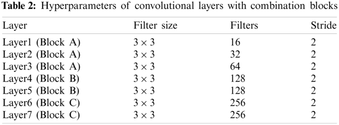
In this paper, a nine-layer convolutional neural network with combination blocks (CNN-CB) was built to identify Chinese sign language, which contains seven convolutional layers with blocks and two fullyconnected layers. As shown in Fig. 10, there are three types of combination blocks: Conv-BN-ReLU-Pooling (Block A), Conv-BN-ReLU (Block B), Conv-BN-ReLU-BN (Block C). Here, Block A is a traditional combination, mainly used to verify and examine the location of pooling operations. Block B is a comparative combination, mainly used to observe the effect of different ReLU functions and difference between whether there is a pooling operation. Block C is an innovative combination that introduces a double BN structure, mainly used to observe the positive significance it brings. In each block, batch normalization, ReLU and pooling all played their respective roles and improved the overall performance. We fine-tuned the hyperparameters to optimize the CNN model. Hyperparameters of convolutional layers with combination blocks was demonstrated in Table 2, here, the values of filters, filter size and stride were listed. Meanwhile, we set padding values as “same”. The probability of dropout rate was set to 0.4 and softmax function was applied.

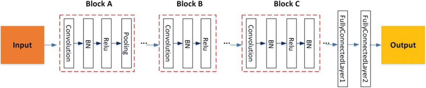
Figure 10: Architecture of the proposed network

3.7 M-Fold Cross-Validation

The larger the amount of data used for model training, the better the trained model will generally be. Therefore, the division of training set and test set means that we cannot make full use of the existing data at hand, so the model effect is affected to a certain extent. Cross-validation is proposed based on this background [52,53].

In M-fold cross validation, the original data is evenly divided into m subspace or folds [54,55]. From the m-folds or groups, for each iteration, one group is selected as validation data and the remaining (m − 1) groups are selected as training data. This process is repeated m times until each group is treated as validation and retained as training data. The final accuracy of the model is calculated by capturing the average accuracy of M-model validation data. A schematic diagram of M-fold cross-validation was given in Fig. 11.

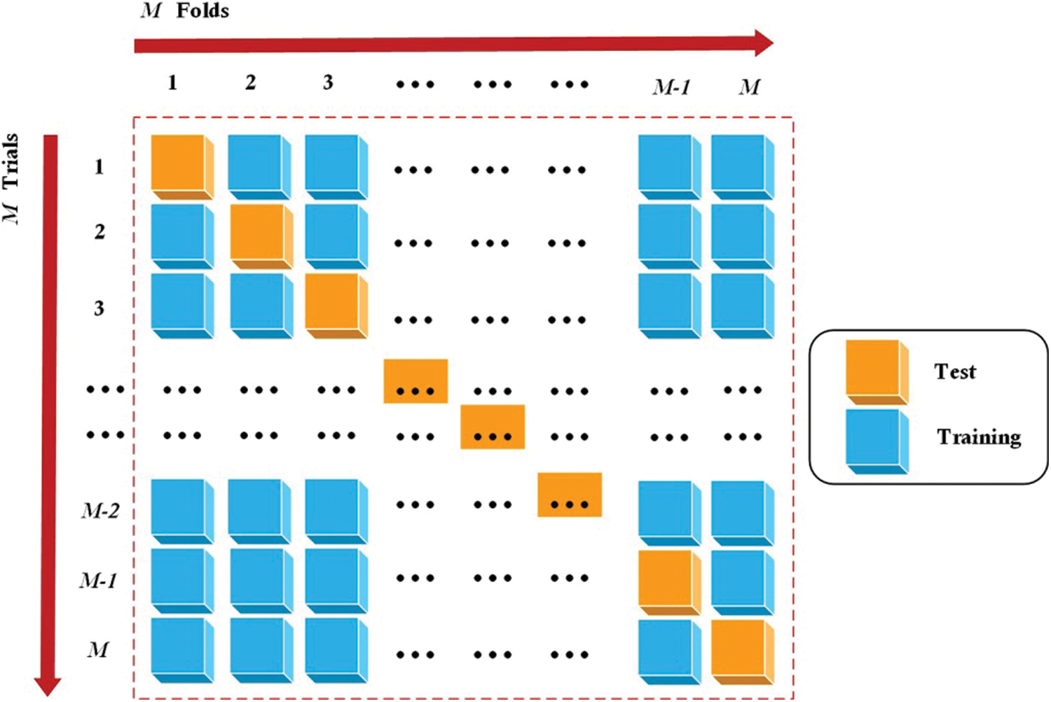
Figure 11: The schematic diagram of M-fold cross-validation

Let's take m = 10 as an example to introduce the steps of the 10-fold cross-validation: i) Divide all data sets into 10 parts; ii) Take one piece of data as test set and use the other nine pieces as training set to train the model, and then calculate the mean square error (MSE) of the model on the test set, denoted as E; iii) The result of an average of 10 trials is the final MSE, the calculation formula is as follows:

CV(m)=1m∑i=1m⁡Ei(13)

The selection of m is the key of the method [56]. The larger m is, the more data of the training set invested each time, and the smaller the deviation of the model. However, the larger m is, the greater the correlation of the training set selected each time is, which will lead to the larger variance of the final test error. In general, as a rule of thumb we usually choose m = 5 or 10. The advantage of cross-validation is that it can obtain as much valid information as possible from limited data, so that it can learn samples from multiple angles and avoid falling into local extremum. In this process, both training samples and test samples have been learned as much as possible.

3.8 Optimization Algorithms

Optimization algorithm is the eye of neural network and the basis of its vigorous development. Stochastic gradient descent (SGD) is one of the most commonly used algorithms to perform optimization, and is also the most commonly used method to optimize neural networks so far. SGD solves the issue of random small batch samples, but it still has some problems such as adaptive learning rate and easy to get stuck in small gradient points. To suppress the oscillation of SGD, inertial control can be used in the process of gradient descent, so momentum is added on the basis of SGD and first-order momentum is introduced, this is the SGD with momentum (SGDM). SGDM alleviates the issue that the local optimal gradient of SGD is 0, which cannot be continuously updated and the oscillation amplitude is too large, but it does not completely solve the problem. When the local gully is deep and the momentum is used up, it will still oscillate back and forth in the local optimal.

The RMSprop approach avoids the problem of continuous accumulation of second-order momentum, resulting in an early end to the training process. It utilizes root mean square prop (RMSprop) to effectively learn multilayer neural networks, and when properly initialized, the neural network suffers much less loss even for deep networks. It is suitable for non-stationary targets (both seasonal and periodic).

Adaptive momentum estimation (Adam) is the integrator of SGDM and RMSprop. SGDM adds first-order momentum on the basis of SGD, and RMSprop adds second-order momentum on the basis of SGD, Adam uses both the first and second order momenta. It basically solves a series of problems of gradient descent mentioned before, such as random small sample, adaptive learning rate, easy to get stuck in a small gradient point and so on.

In general, SGD is the most common optimizer, and Adam and RMSprop are the two most influential adaptive stochastic algorithms for training deep neural networks. While SGD has no acceleration effect, momentum is a modified version of SGD, adding the momentum principle. The latter RMSprop is again an upgrade to momentum, and Adam is again an upgrade to RMSprop. Adam has a fast convergence speed, while SGDM is slower, but they can converge to a good point eventually. Adam performed best in the training set, but SGDM did best in the verification set. It can be seen that SGDM is better than Adam in training set and verification set consistency. However, in some cases, the performance of Adam seems to be less than RMSprop, so it is not that the more advanced the optimizer, the better the results. So, it is necessary to choose the appropriate algorithm according to the characteristics and requirements of the data set.

4  Experiments, Results, and Discussions

4.1 Experimental Configuration

This experiment was carried out on a platform with CPU of Core i7, memory of 16 GB and Windows 10 operating system. Experimental configuration and related parameters were set as follows: InitialLearnRate was defined as 0.01, MiniBatchSize was defined as 256, LearnRateDropPeriod was set to 10, LearnRateDropFactor was set to 0.1, meanwhile, we ordered the maximum epoch as 30 and tested three training algorithms: SGDM, RMSProp and Adam, respectively. Overall accuracy (OA) was adopted to evaluate the results of experiment, which denotes the proportion of correct-classify samples in all samples.

4.2 Statistical Results

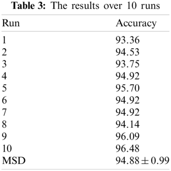
Our CNNCB model was employed via 10 runs with 10-fold cross-validation, in which three combination blocks: Conv-BN-ReLU-Pooling, Conv-BN-ReLU, Conv-BN-ReLU-BN were adopted. The results over 10 runs are displayed in Table 3. As can be seen, the MSD (mean and standard deviation) is 94.88 ± 0.99%, the highest accuracy reaches to 96.48% and the lowest accuracy is about 93.36%, respectively. It indicates that the results are steady and effective.

4.3 Pooling Method Comparison

In the experiment, we replaced the average pooling (AP) in block A with max pooling (MP) method. Meanwhile, we kept all the other settings unchanged. The results of 10 runs of max pooling are as follows: 92.97%, 93.75%, 92.58%, 94.14%, 94.14%, 94.14%, 93.75%, 93.75%, 94.53%, and 95.70%. The MSD of max pooling is 93.95 ± 0. 85%. The comparison against AP and MP is shown in Fig. 12. It demonstrates that AP is relatively superior to MP in term of identification accuracy.

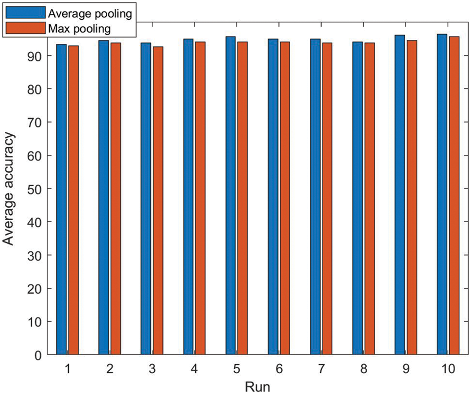
Figure 12: The comparison against AP and MP

4.4 Dropout Comparison

According to existing experience, the dropout rate is generally set to 0.5. Therefore, we varied the dropout rate around 0.5 as the comparison. The results of 10 runs under different dropout rates are demonstrated in Fig. 13. It can be seen that when the dropout rate is 0.4, the overall accuracy rate reaches its peak, which gives the best performance. Setting the dropout rate to 0.5 does not work well in this experiment. When the dropout rate is 0.5, 0.6 and 0.7, the overall accuracy are 91.72 ± 0.80%, 93.59 ± 1.72% and 91.88 ± 1.01%, respectively. Among them, the result of setting dropout rate to 0.6 is close to the highest accuracy rate. Therefore, the optimal dropout rate is 0.4.

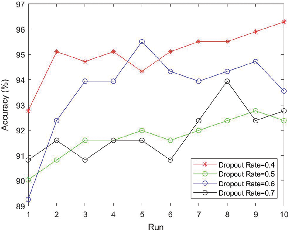
Figure 13: Effect under different dropout rates

4.5 ReLU vs. Leaky ReLU

In the experiment, we compared the effects of ReLU and Leaky ReLU. The results were presented in Fig. 14. It can be observed that in ten runs Leaky ReLU is superior to ReLU. ReLU reaches average accuracy of 92.30 ± 0.59%, which is low than the average accuracy of Leaky ReLU about 2.5 percentage point. The reason is that ReLU cannot fix the issue of zero-downside while Leaky ReLU can solve the issue of dead neurons by adopting the small negative gradient flow. Thus, the data distribution was corrected and the information of negative axis will not be lost, which enhances performance and achieves better accuracy.

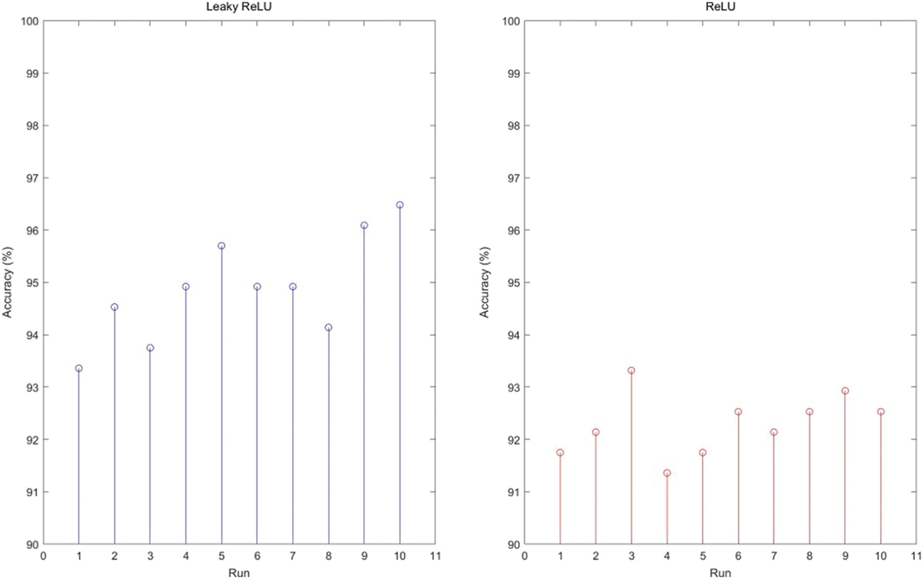
Figure 14: Leaky ReLU vs. ReLU

4.6 Block Comparison

In this experiment, we compared our combination blocks method with other four model of combination blocks: 2(Block A-Block B)-1(Block B)-2(Block C), 3(Block A)-2(Block B)-1(Block C), 2(Block A)-1(Block C)-1(Block A)-2(Block B), and 3(Block A)-4(Block B). The results were presented in Table 4. It can be observed that our method achieved superior performance than all other methods. Meanwhile, we can draw three conclusions: (i) After introducing the Batch Normalization technology twice in one block, the overall performance and effect are much better. That is, Block C played a more significant role. As can be seen in Table 3, Model1 reached MSD 94.88 ± 0.99%, which is superior to Model5 87.42 ± 1.41%. (ii) The double BN structure should be placed in the back convolutional layer. We can observe that Block C is set to last position in Model1, Model2 and Model3. Thus, the performance brought by this structure is significantly better than the way that Block C is placed in the middle in Model4. (iii) Put the pooling operation in front. That is, there should be no other modules before Block A. Obviously, the performance degradation of Model2 and Model4 is mainly due to the appearance of other blocks before Block A.

The reason why our proposed method is the best among all five methods lies in the following two points: (i) The batch normalization technology was employed, which normalized the latest inputs with a mini batch, thus, the input layer was evenly distributed. The introduction of dual BN technology strengthens this effect, which can better prevent the problem of gradient disappearance and accelerate learning convergence. (ii) The pooling layer can be used to achieve dimensionality reduction and reduce the overfitting and computational burden of activation maps due to too many features. Put the pooling operation in the front convolutional layer to achieve dimensionality reduction as soon as possible, and the effect is better. In addition, pooling also helps to maintain invariance-to-translation.

4.7 Comparison to State-of-the-Art Methods

In this experiment, our CNN-CB method was compared with some traditional machine learning methods: HCRF [57], HMM [58], SVM-HMM [59], GLCM-MGSVM [60], WE+SVM [61], HMI-RBF-SVM [62], FSVM [63], WE-kSVM [64]. As can be seen in Table 5, our method is eventually superior to all eight state-of-the-art methods. Additionally, some modern CNN methods: 6L CNN-LReLU [21], eight-Layer CNN [22], AlexNet-DA-Adam [65], 9L-CNN [66], CNN7-DA [67] were compared with our method. The results were displayed in Table 6. It can be observed that our CNN-CB method also achieved superior performance. Intuitively shown in Fig. 15, our method has achieved a significant lead.

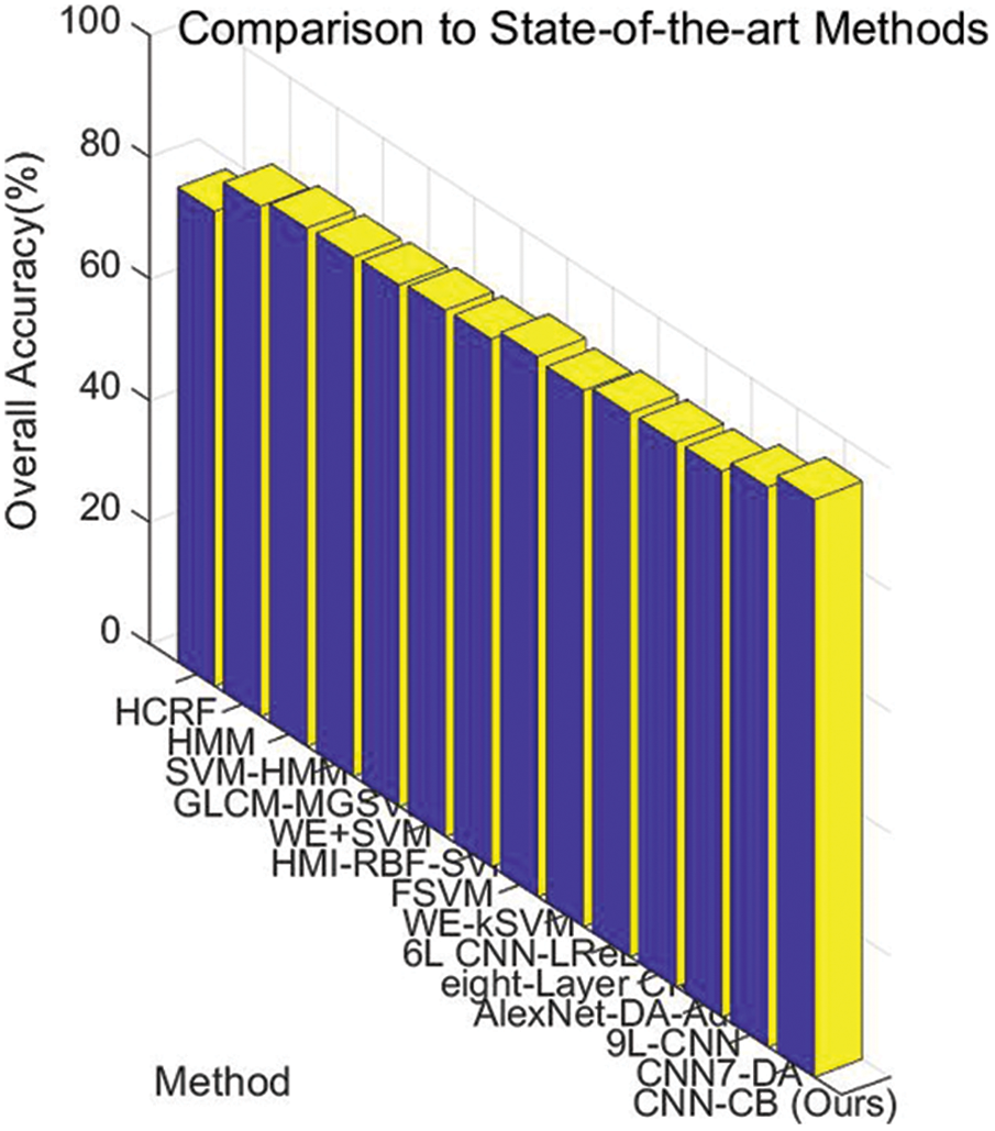
Figure 15: Comparison to state-of-the-art methods

The reason why our CNN-CB method gives the best overall accuracy among all Chinese sign language identification approaches lies in one point. An optimized CNN with combination blocks, including advanced techniques such as batch normalization, pooling, Leaky ReLU, dropout, was employed. Among them, BN can evenly distribute the input layer and avoid gradient disappearance. Adopting dual BN promotes the effect and speeds up learning convergence. Pooling operation achieves dimensionality reduction, which decreases burden of computation and reduces the overfitting. The utilization of Leaky ReLU can fix the issue of “dead neurons” and correct the data distribution. The dropout technology can not only shrink the scale of neural network, but also ameliorate the ability of generalization. Particularly, different combinations of blocks: Conv-BN-ReLU-Pooling, Conv-BN-ReLU, Conv-BN-ReLU-BN enhance performance and achieve better accuracy.

5  Conclusion

In this study, an optimized convolutional neural network with combination blocks was proposed to identify Chinese sign language. Three different combinations of blocks: Conv-BN-ReLU-Pooling, Conv-BN-ReLU, Conv-BN-ReLU-BN were adopted, including batch normalization, pooling, ReLU and dropout techniques. The results displayed that our CNN-CB method gained an overall accuracy of 94.88 ± 0.99%, which is superior to thirteen state-of-the-art methods: eight traditional machine learning approaches and five modern convolutional neural network approaches.

Meanwhile, there are some weaknesses in our approach. First of all, our dataset including 1320 images is relatively insufficient, which needs to be extended further more. Next, more probable combinations can be tested and more advanced technologies can be tried.

Thus, in the future, more Chinese sign language images should be obtained to avoid over-fitting and improve the training performance. Furthermore, research on Chinese sign language video recognition should be on the agenda. Data augmentation technique and optimized training models should be focused on. Moreover, some advanced deep learning network models such as ResNet, DenseNet, SqueezeNet can be tried.

Funding Statement: This work was supported from The National Philosophy and Social Sciences Foundation (Grant No. 20BTQ065).

Conflicts of Interest: The authors declare that they have no conflicts of interest to report regarding the present study.

This work is licensed under a Creative Commons Attribution 4.0 International License, which permits unrestricted use, distribution, and reproduction in any medium, provided the original work is properly cited.