Computer Modeling in Engineering & Sciences

DOI: 10.32604/cmes.2022.020394

ARTICLE

Low Carbon Economic Dispatch of Integrated Energy System Considering Power Supply Reliability and Integrated Demand Response

Jian Dong, Haixin Wang, Junyou Yang*, Liu Gao, Kang Wang and Xiran Zhou

School of Electrical Engineering, Shenyang University of Technology, Shenyang, 110870, China
*Corresponding Author: Junyou Yang. Email: junyouyang@sut.edu.cn
Received: 20 November 2021 Accepted: 14 December 2021

1  Introduction

In recent years, with the development of the world economy and the increasing depletion of fossil fuels, the problem of insufficient energy supply has become increasingly prominent [1,2]. On 05 March, 2021, China pointed out in the government work report that CO2 emissions would be at the peak by 2030 and achieve carbon neutrality by 2060. As an important carrier for the development of the energy internet, the integrated energy system (IES) can promote the coordination and complementation of various energy sources [3,4]. Meanwhile, the IES has made significant contributions to building clean, low-carbon and efficient energy systems. However, with the deepening of energy coupling, the IES is confronted with enormous challenges due to fluctuating wind and PV power outputs and the uncertainty of multi-energy demands [5–7].

The operation economy and power supply reliability are two essential factors in energy management and optimization of the IES [8–10]. Power supply reliability is an important indicator to measure the stable operation of the power grid, and economic benefit is an important goal in the development of IES [11].

Regarding the low-carbon operation of IESs, Wang et al. [12] proposed an optimal scheduling model based on the carbon trading mechanism. IES operators can purchase or sell carbon quotas in the carbon trading market. The results show that considering carbon trading can reduce the operation cost of the IES. Zhai et al. [13] proposed an economic dispatch method for low-carbon power system considering the uncertainty of electric, thermal and cold loads. Yang et al. [14] proposed an optimal scheduling model for the combination of the microturbine (MT) and power to gas (P2G) units. The typical load scenarios are obtained by scenario generation and reduction techniques to improve wind power consumption and reduce carbon dioxide emissions. Although the above literature can realize the low-carbon operation of the system, the flexible resources of the demand side are not considered.

Considering integrated demand response (IDR) in IES can promote renewable energy consumption and reduce carbon emissions. Bahrami et al. [15] established a power system scheduling model considering demand response (DR) resources and carbon trading and verify its effectiveness in promoting wind power consumption and reducing carbon emissions. Zeng et al. [16] introduced the split-flow carbon capture power plant and DR into the IES to achieve low carbon.

Although remarkable results are achieved in the economic dispatch of the IES, the above models are solved by traditional methods, and the optimization effect is dependent on the prediction accuracy of sources and loads. With the development of the artificial intelligence (AI) technique, reinforcement learning (RL) has been paid more attention to the optimal control of power system [17–20]. The RL model can accumulate experience and improve policies by continuous interaction with the environment. In particular, the deep reinforcement learning algorithm combining deep neural network and reinforcement learning is of better adaptive learning ability and optimized decision-making ability for nonconvex and nonlinear problems [20–22]. In [23], microgrid (MG) real-time energy management based on deep reinforcement learning was proposed, and MG energy management is described as a Markov decision process (MDP) to minimize the daily operating cost. In [24], the energy management of IES was described as a constrained optimal control problem and solved by the asynchronous advantage actor critic algorithm.

The above studies provided the foundation for the application of the DRL approach in the IES. However, most of the above models only consider the economy and security of IES, without consideration of carbon dioxide emissions and other indicators in the system. In addition, in the face of collaborative optimization of multi-energy and energy storage, the model training may be time-consuming and prone to non-convergence.

This paper proposes a TD3-based integrated energy system source-load coordination optimization scheduling framework. Firstly, a combined optimization model of combined thermal and power (CHP), power to gas (P2G) and carbon capture system (CCS) is established, which can realize thermal-power decoupling and reduce carbon emissions. Secondly, the multi-objective optimization problem of IES is described as a Markov decision process, the environmental model of IES is established, and the action space, state space and reward function of the agent are designed. Finally, the low-carbon economic dispatch problem is solved by the twin delayed deep deterministic policy gradient (TD3), and the convergence ability and stability of this method are analyzed. Finally, the effectiveness of this method in the low-carbon economic dispatch of the IES is validated.

2  IES Model and Problem Description

Low-carbon operation optimization of the IES aims to improve the economic and environmental benefits of the system with the constraint of safe operation of the system. This paper studies a multi-objective optimization problem with optimal economic cost, carbon emissions, and reliability of system operation. The structure of the IES studied in this paper is shown in Fig. 1. The power grid includes combined thermal and power (CHP), carbon capture system (CCS), wind power, photovoltaic, battery storage (BS) and electricity load. The gas network comprises the natural gas station, gas storage (GS) and gas load. The thermal supply network mainly consists of thermal storage (HS) and thermal load. The energy conversion equipment mainly includes gas turbine, P2G and MT.

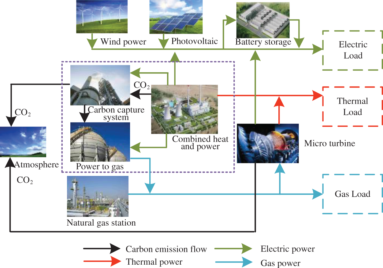
Figure 1: Structure diagram of the IES

2.1 IES Equipment

(1) CHP-CCS-P2G (CCP) Mathematical Model

The CHP units provide electric power and thermal power in the IES. The CHP has high carbon emissions and thermoelectric coupling characteristics, which causes severe environmental pollution. Therefore, according to the literature [25], the optimization model of CCP is established to reduce carbon emissions and improve the economic benefits of the IES. The principle of the CCP is shown in Fig. 2. P2G converts the electric power generated by CHP into natural gas, which strengthens the connection of the power-thermal-gas system and reduces the power output of CHP. The electric power consumed by P2G and CCS is directly taken from electric power generated by CHP. To reduce carbon emissions of CHP and carbon source cost of P2G, the CO2 is captured by CCS, and transmitted to P2G for recycling.

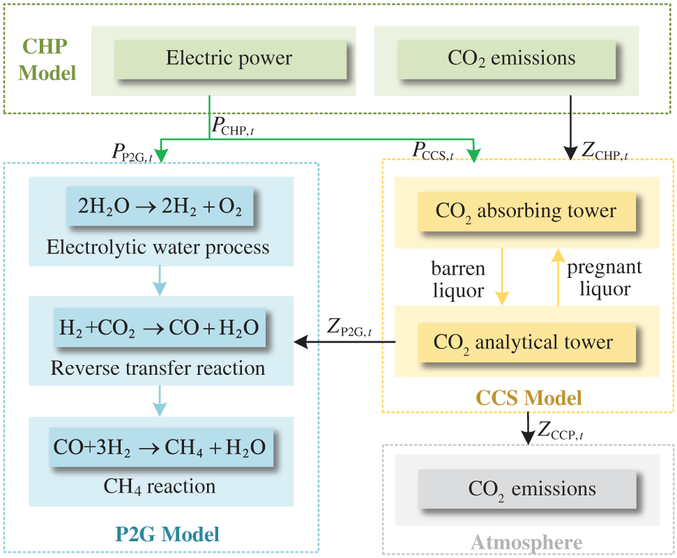
Figure 2: The principle of CCP combined optimization model

The electric power output of the CCP can be calculated by Eq. (1).

PCCP,t=PCHP,t−PP2G,t−PCCS,t, (1)

where PCCP,t is the electric power output of the CCP at time t, PCHP,t is the electric power generated by CHP, PP2G,t is the electric power consumed by P2G, PCCS,t is the electric power of CCS.

The gas power output of the CCP can be calculated by Eq. (2).

GCCP,t=GP2G,t=ηP2GPP2G,t, (2)

where GCCP,t is the gas power output of the CCP at time t, GP2G,t is the gas power output of the P2G, ηP2G is the conversion efficiency of P2G.

The electric power and ramp rate constraints of CCP can be described by Eqs. (3) and (4).

PCCPmin=PCHPmin−PP2Gmax−PCCSmax≤PCCP,t≤PCHPmax−PP2Gmin−PCCSmin=PCCPmax, (3)

ΔPCCPmin=ΔPCHPmin−ΔPP2Gmax−ΔPCCSmax≤PCCP,t+1−PCCP,t≤ΔPCHPmax−ΔPP2Gmin−ΔPCCSmin=ΔPCCPmax, (4)

where PCCPmin,PCHPmin,PP2Gmin and PCCSmin are the lower limits of electric power of CCP, CHP, P2G and CCS, PCCPmax,PCHPmax,PP2Gmax and PCCSmax are the upper limits of electric power of CCP, CHP, P2G and CCS, ΔPCCPmin,ΔPCHPmin,ΔPP2Gmin and ΔPCCSmin are the lower limits of electric power ramp rate of CCP, CHP, P2G and CCS, ΔPCCPmax,ΔPCHPmax,ΔPP2Gmax and ΔPCCSmax are the upper limits of electric power ramp rate of CCP, CHP, P2G and CCS.

The thermal power and ramp rate constraints of CCP can be described by Eqs. (5) and (6).

HCCPmin=HCHPmin≤HCCP,t≤HCHPmax=HCCPmax, (5)

ΔHCCPmin=ΔHCHPmin≤HCCP,t+1−HCCP,t,≤ΔHCHPmax=ΔHCCPmax, (6)

where HCCP,t + 1 and HCCP,t are the thermal power output of the CCP at time t and t + 1, HCCPmin and HCHPmin are the lower limits of thermal power of CCP and CHP, HCCPmax and HCHPmax are the upper limits of thermal power of CCP and CHP, HCCPmin andΔHCHPmin are the lower limits of thermal power ramp rate of CCP and CHP, ΔHCCPmax and ΔHCHPmax are limits of thermal power ramp rate of CCP and CHP.

The gas power and ramp rate constraints of CCP can be described by Eqs. (7) and (8).

GCCPmin=GP2Gmin≤GCCP,t≤GP2Gmax=GCCPmax, (7)

ΔGCCPmin=ΔGP2Gmin≤GCCP,t+1−GCCP,t≤ΔGP2Gmax=ΔGCCPmax, (8)

where GCCP,t+1 and GP2G,t are the gas power output of the CCP at time t and t+1, GCCPmin and GP2Gmin are the lower limits of gas power of CCP and P2G, GCCPmax and GP2Gmax are the upper limits of gas power of CCP and P2G, ΔGCCPmin and ΔGP2Gmin are the lower limits of gas power ramp rate of CCP and P2G, ΔGCCPmax and ΔGP2Gmax are the upper limits of gas power ramp rate of CCP and P2G.

(2) MT Mathematical Model

MT driven by natural gas is the essential equipment of the IES [25]. The mathematical model of MT is shown by Eqs. (9) and (10).

PMT,t=GMT,t⋅ηMT, (9)

HMT,t=GMT,t⋅(1−ηMT−ηloss), (10)

where PMT,t and HMT,t are the electric and thermal power of MT at time t, GMT,t is the natural gas consumption power of MT, ηMT is the power generation efficiency of MT, ηloss is the energy loss coefficient of MT.

The power and ramp rate constraints of MT can be described by Eqs. (11)–(14).

PMTmin≤PMT,t≤PMTmax, (11)

HMTmin≤HMT,t≤HMTmax, (12)

ΔPMTmin≤PMT,t−PMT,t−1≤ΔPMTmax, (13)

ΔHMTmin≤HMT,t−HMT,t−1≤ΔHMTmax, (14)

where PMTmin and PMTmax are the lower limits and upper limit of electric power of the MT, HMTmin and HMTmax are the lower limits and upper limits of thermal power of the MT, ΔPMTmin and ΔPMTmax are the lower limits and upper limit of electric power ramp rate of the MT, ΔHMTmin and HMTmax are the lower and upper limits of thermal power ramp rate of MT.

(3) Energy Storage Battery Model

The mathematical model of battery storage is expressed by Eqs. (15)–(17) [8].

SOCt+1=SOCt+ach,tηchPBS,ch,tQBSΔt+ax,disch,tPBS,disch,tηdischΔt, (15)

ach,t,adisch,t={0,1},∀t∈T, (16)

ach,t∧adisch,t=0,∀t∈N, (17)

where SOCt+1 and SOCt are the states of charge of the BS at time t + 1 and t, PBS,ch,t and PBS,disch, are the charging and discharging power of BS at time t (PBS,ch,t ≥ 0, PBS,disch,t ≤ 0). QBS is the capacity of BS, ηch and ηdisch are the charging and discharging efficiency of BS, Δt is the time interval, ach,t and adisch,t are the charging and discharging state parameters, ach,t = 1 represents the charging operation of the BS at time t, and similarly, adisch,t = 1 represents the discharging operation of the energy BS at time t.

The energy storage equipment is limited by the following charging and discharging power constraints and capacity constraints in Eqs. (18)–(21).

SOCmin≤SOCt≤SOCmax, (18)

0≤PBS,ch,t≤PBS,chmax, (19)

0≥PBS,disch,t≥PBS,dischmax, (20)

SOC1=SOCT, (21)

where SOCmin and SOCmax are maximum and minimum SOC values of the BS, PBS,chmax and PBS,dischmax are maximum charging and discharging power of the BS, SOC1 and SOCT are the initial and final values of the BS.

2.2 IES Model

(1) Electric Network Model

The power flow constraints can be formulated by Eq. (22) [18].

{Pi,t=Ui,t∑j∈iUj,t(Gijcos⁡θij,t+Bijsin⁡θij,t)Qi,t=Ui,t∑j∈iUj,t(Gijsin⁡θij,t−Bijcos⁡θij,t), (22)

where Pi,t is the active power of node i at time t, Qi,t is the reactive power of node i at time t, Ui,t and Uj,t are the voltage values of nodes i and j, Gij is the electric conductance between nodes i and j, Bij is the electrical susceptance between nodes i and j, θij,t is the phase angle difference between nodes i and j.

(2) Natural Gas Network Model

The mathematical description of the natural gas network mainly includes pipe flow, compressor and gas flow models. The pipe flow equation of natural gas is obtained by Eqs. (23) and (24).

Gmn=Zmnσmnσmn(Φm2−Φn2), (23)

σmn={1,Φm>Φn−1,Φm≤Φn, (24)

where Gmn is the steady-state flow rate of natural gas pipeline mn, Zmn is the pipeline constant, which depends on various factors (e.g., inner diameter, length, friction coefficient and temperature of the pipeline), Φm and Φn are the pressure of nodes m and n, σ is the flow direction coefficient of natural gas.

The mathematical model of the compressor can be described by Eq. (25).

Pcom=ZcomGcom,mn[(Φn/Φm)Dcom−1], (25)

where Pcom is the electric power of the compressor, Zcom is the compression ratio, Gcom,mn is the gas flow through the compressor, Dcom is the compressor parameter.

The gas flow constraints of the natural gas network can be described by Eqs. (26) and (27).

Zcommin≤Zcom=Φn/Φm≤Zcommax, (26)

Φnmin≤Φn≤Φnmax, (27)

where Zcommin and Zcommax are the lower and upper limits of the compression ratio of the compressor, Φnmin and Φnmax are the lower and upper limits of natural gas pressure at node n.

(3) Thermal Network Model

The thermal network model mainly includes the hydraulic model and thermodynamic model [26]. The hydraulic model is described by Eq. (28).

{AkM=MkBH=0, (28)

where Ak is the node-to-branch incidence matrix of the thermal network, M is the water flow matrix of the pipeline, and Mk is the water flow matrix of the node k, B is the loop-to-branch incidence matrix of the thermal network, H is the pipeline pressure loss matrix.

The thermodynamic model of the thermal supply network is expressed by Eq. (29).

{Hk=CHmk(Tk,s−Tk,o)Tk,out∑u∈Emu=∑l∈YmlTkl,inTend=(Tstart−Tg)e−εL/cHm+Tg, (29)

where Hk is the thermal power of node k of the thermal network, CH is the thermal capacity of water, mk is the water flow out of node k, Tk,s and Tk,o are the temperature of water flowing into and out of node k, E and Y are the upstream and downstream pipeline sets of node k, mu and ml are the water flow of pipelines u and l, Tk,out is the initial temperature of the downstream pipeline, Tkl,out is the terminal temperature of downstream pipeline l, Tstart and Tend are the initial and terminal temperature of the pipeline, Tg is the ambient temperature, ɛ is the thermal transfer coefficient of the pipeline, and L is the pipeline length.

2.3 IDR Model

As a flexible resource, IDR is conducive to achieving low-carbon economic operation and improving the operation reliability of the IES. IDR can reduce energy demand during peak load periods by reducing, converting and shifting electric power demand. Renewable energy is used to replace high carbon emission units.

The consumption of transferable electric load in the peak demand period is shifted to other periods. The sum of all transferred load is within a certain little range to satisfy the load demand. The transferable load complies with the following operating constraints:

{PLoad,i,t′=PLoad,i,t−PTra,i,tPLoad,i,t+υ′=PLoad,i,t+υ+PTra,i,t, (30)

δTra,iminPLoad,i,t≤PTra,i,t≤δTra,imaxPLoad,i,t, (31)

where P′Load,i,t and P′Load,i,t+υ are the electric load of node i after transfer at time t and t+υ, PLoad,i,t and PLoad,i,t+υ are the electric load of node i before transferring at time t and t+υ, PTra,i,t is the electric load of node i transferred from time t to time t+υ, δTra,imin and δTra,imax are the maximum and minimum proportional coefficients of the transferable load of node i.

Interruptible loads comply with the following operating constraints in Eqs. (32) and (33).

P′Load,i,t=PLoad,i,t−PInt,i,t, (32)

δInt,iminPLoad,i,t≤PInt,i,t≤δInt,imaxPLoad,i,t, (33)

where PInt,i,t is the electric load of node i interrupted at time t, δInt,imin and δInt,imax are the maximum and minimum proportionality coefficients of the interruptible load of node i.

Users can convert peak electric load demand to other energy sources. The convertible load model is shown by Eqs. (34) and (35).

PCon,i,t=ϕPGGCon,m,t+ϕPHHCon,k,t, (34)

δCon,iminPLoad,i,t≤PCon,i,t≤δCon,imaxPLoad,i,t, (35)

where PCon,i,ta is the reduced electric load of power grid node i at time t after conversion, GCon,m,ta is the increased gas load of gas network node m at time t after conversion, HCon,k,ta is the increased thermal load of thermal supply network node k, δCon,imin and δCon,imax are the maximum and minimum proportionality coefficients of the convertible load of node i.

2.4 Objective Function

In this paper, a low-carbon dispatching model of the IES is established to minimize the total cost of the system. The objective function is expressed by Eq. (36).

F=min(CO+CC+CCWind+CCPV+CIDR+CLS), (36)

where CO is the system operating cost, CC is the CO2 emission cost, CQF is the wind curtailment cost, CQG is the PV curtailment cost, CIDR is the IDR cost, and CLS is the load shedding cost.

(1) System Operating Cost

The system operating cost includes CCP operating cost and MT operating cost, which can be described by Eq. (37).

{CO=CCCP+CMTCCCP=∑x=1N[(aCHP,xPCHP,x,t2+bCHP,xPCHP,x,t+cCHP,x)+(aCCS,xPCCS,x,t+bCCS,xZCCS,x,t)+(aP2G,xPP2G,x,t+bP2G,xZP2G,x,t)]CMT=∑x=1NaMT,xPMT,x,t, (37)

where CCCP and CMT are the operating costs of CCP and MT, aCHP,x, bCHP,x and cCHP,x are the operating cost coefficients of CHP, aCCS,x and aP2G,x are the operating cost coefficients of CCS and P2G, ZCCS,x,t is the carbon emissions captured by CCS at time t, ZP2G,x,t is the carbon consumed by P2G x at time t, bCCS,x is the cost coefficient of CO2 capture of CCS, and bP2G,x is the cost coefficient of CO2 purchase of P2G.

(2) Carbon Trading Cost

The carbon emissions of the system come from CHP and MT, and the part of them is absorbed by CCS. The carbon trading cost can be described by Eq. (38).

CC=λ∑x=1N(ZCHP,x,t+ZMT,x,t−ZCCS,x,t−ZQ,t), (38)

where λ is the carbon trading cost coefficient, ZCHP,x,t is the carbon generated by CHP x at time t, ZMT,x,t is the carbon generated by MT, and ZQ,t is the carbon emission quota.

(3) Wind Curtailment Cost

The wind curtailment cost can be described as Eq. (39).

CCWind=aCWindPCWind,t, (39)

where aCWind is the penalty cost coefficient of wind power curtailment, PCWind,t is the wind power curtailment at time t.

(4) PV Curtailment Cost

The PV curtailment cost can be calculated by Eq. (40).

CCPV=aCPVPCPV,t, (40)

where aCPV is the penalty cost coefficient of PV curtailment, PCPV,t is the PV curtailment at time t.

(5) IDR Cost

The IDR cost is obtained by Eq. (41).

CIDR=∑i∈ΩIDR(aTraPTra,i,tab+aIntPInt,i,ta+aConPCon,i,ta) (41)

where ΩIDR is the set of nodes participating in demand response, aTra, aInt and aCon are the cost coefficients of transferable load, interruptible load and convertible load.

(6) Power Supply Reliability

To improve the power supply reliability of the IES, this paper uses the loss of power supply probability (LPSP) as the standard to measure the power supply reliability. The power supply reliability is calculated by Eq. (42).

LPSPt=PLS,tPLoad,t, (42)

where PLS,t is the load shedding power at time t.

The load shedding cost can be calculated by Eq. (43).

CLS=aLSPLS,t, (43)

where aLS is the load shedding cost coefficient.

2.5 Objective Function

To meet the demand of electric-gas-heat load in each operation period, the system balance constraints are given by Eq. (44).

{PCCP,i,t+PPV,i,t+PWind,i,t+PBS,disch,i,t+PBS,ch,i,t=PLoad,i,t−PTra,i,t−PInt,i,t−PCon,i,t−PLS,i,tGG,m,t+GCCP,m,t−GMT,m,t=GLoad,m,t+GCon,m,tHCCP,k,t+HMT,k,t=HLoad,k,t+HCon,k,t, (44)

where PPV,i,t and PWind,i,t are PV and wind energy output power of power grid node i at time t, GG,t is the purchased gas power of gas network node m, while PLoad,i,t, GLoad,m,t and HLoad,k,t are electric load, gas load and heat load.

3  Deep Reinforcement Learning Model for Low Carbon Economic Dispatch of the IES

In this paper, the multi-objective optimization problem of low-carbon economic dispatch of the IES is solved by the DRL method. In this section, the optimal problem of low-carbon economic dispatch of the IES is transformed into a DRL framework and solved by the TD3 algorithm.

3.1 Problem Transformation

Reinforcement learning is the process of interacting with the environment, obtaining feedback, updating strategy, iterative until learning the optimal strategy [23]. This environmental interaction is described by the Markov decision process (MDP), which consists of five elements: state space S, action space A, transfer function T, reward function P and discount factor γ.

(1) State Space

The observed state of the IES is shown in Eq. (45), including the state of charge SOCt of battery storage, wind power output Pwind,t, PV output PPV,t, electric load PLoad,t, gas load GLoad, heat load HLoad,t and time t.

st=(SOCt,PWind,t,PLoad,t,GLoad,t,HLoad,t,t). (45)

(2) Action Space

The action space of the IES is shown in Eq. (46), including electric power output PCCP,t and gas power output GCCP,t of the CCP, electric power PMT,t of gas turbine, output power PBS,t of energy storage battery, and electric power PIDR,t of the IDR.

at=(PCCP,t,GCCP,t,PMT,t,PBS,t,PIDR,t). (46)

(3) Reward

The reward function is set to guide the agent to acquire the maximum cumulative reward from the current action. Therefore, as the reinforcement learning agent generally employs maximizing cumulative reward, the reward is a negative value of the objective function. The reward function can be described by Eq. (47).

Rt=−(CO+CC+CCWind+CCPV+CIDR+CLS)+r0, (47)

where r0 is a manually set constant, which is used to ensure that the cumulative reward of the agent changes from a negative value to a positive value in the learning process.

The punishment reward mainly includes two parts, agent action amplitude penalty and agent action change rate punishment, Which can be shown by Eq. (48).

χt=∑t=1T∑ai[κ11,imax(ai,t+1−ai,t−a11,i,max,0)+κ12,imax(ai,t−ai,t+1−ai,12,min,0)+κ21,imax(ai,t−ai,21,max,0)+κ22,imax(ai,t+1−ai,22,min,0)], (48)

where κ11,i, κ12,i are the upper and lower penalty coefficients of the agent’s climbing action, a11,i,max, ai,12,min are the upper and lower climbing limits of the action, κ21,i, κ22,i are the upper and lower penalty coefficients of the agent’s action, ai,21,max, ai,22,min are the upper and lower limits of the action.

3.2 Problem Solving Based on TD3 Algorithm

In this paper, the multi-objective optimization problem of low-carbon economic dispatch of the IES is solved by the DRL method. In this section, the optimal problem of low-carbon economic dispatch of the IES is transformed into a DRL framework and solved by the TD3 algorithm. TD3 is a DRL algorithm based on the actor-critic framework and DDPG. The principle of the TD3 algorithm is shown in Fig. 3. The actor-critic framework adopts two neural networks. The actor generates action according to state, and critic inputs state and action to generate Q value and learns reward and punishment mechanism to evaluate the behavior selected by the actor. The agent updates relevant parameters in the continuous state by updating the strategy of the actor and achieves the single-step update effect.

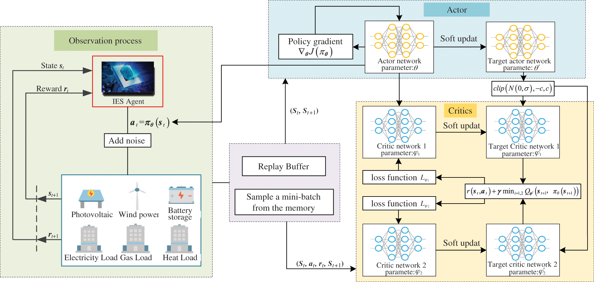
Figure 3: The principle of the TD3 algorithm

In the DDPG algorithm, the actor generates deterministic actions according to the policy function at=πθ(st). The parameter of the actor-network is θ, and the optimization objective can be described by Eqs. (49) and (50) [17].

J(πθ)=E[Q(st,πθ(st))], (49)

∇θJ(πθ)=∇θE[Q(st,at)]=E[∇θπθ(st)∇aQ(st,at)|at=πθ(st)], (50)

where Q(st,at) is the action-value function, which indicates the expected reward value of the selected action at in the state st.

The critic is a Q function, which is used to fit the state-action value. The critic evaluates the action in the current state and provides gradient information for the actor. The target is calculated by Eq. (51).

yt=r(st,at)+γQφ′(st+1,πθ(st+1)) (51)

where Qφ′ is the target Q network, yt is the target value of the critic network.

In DDPG, there is an overfitting phenomenon of the Q network, leading to the overestimation of the Q value. Under this circumstance, the policy network will affect the final performance by learning wrong information. TD3 algorithm can solve the overestimation problem of DDPG, restrict the overfitting of the Q network and reduce the deviation. Therefore, based on the DDPG framework, the improvements of TD3 are as follows:

(1) Clipped double-Q learning under actor-critic framework [27]. In the DDPG algorithm, both target actor-network and target critic network adopt the “soft update” method, which makes the actual network similar to the target network. It is difficult to separate the action selection and policy evaluation. Therefore, in the TD3 algorithm, the target value is obtained by clipping double-Q learning, and the Q value is constrained by two Q networks. Besides, corresponding minimum Q value in two Q networks are adopted to calculate the target Q value. According to the actor network πθ, the target value yt2 of the critic network Qφ2 is equal to yt1 as shown in Eq. (52).

yt1=r(st,at)+γmini=1,2Qφ′(st+1,πθ(st+1)). (52)

(2) Smoothen the target action. In the continuous action space, it is usually expected that the same actions can have similar values [25]. Therefore, the action output of the agent is smoothened by adding random noise to the target action. The value function is updated by Eqs. (53) and (54).

yt=r(st,at)+γmini=1,2Qφ′(st+1,πθ(st+1)+ε), (53)

ε∼clip(N(0,σ),−c,c), (54)

where ɛ is the random noise.

(3) Delay the update of the policy network. Policy network cannot be trained according to poor performance Q network evaluation [28]. Therefore, in TD3, the actor is updated after the critic is updated for n times. The target network parameters are updated by Eq. (55).

θ′=(1−τ)⋅θ′+τθ,φ′=(1−τ)⋅φ′+τφ, (55)

where τ is the soft update rate.

4  Case Study

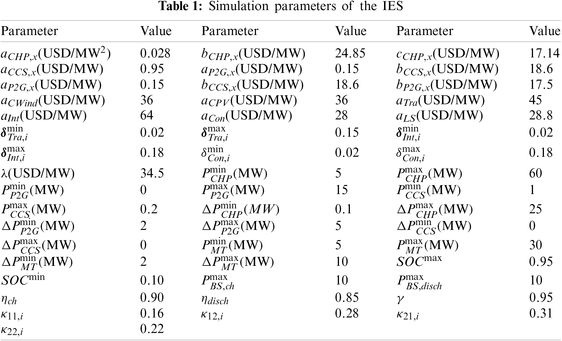
The simulation environment is established in the Gym toolkit of Open AI. The simulation structure of the IES in this paper is composed of IEEE 39-bus power system, 6-bus heating system and 20-bus natural gas system [1]. The natural gas price is 33 C//m. TD3 algorithm uses the neural network to fit actor and critic network. The number of hidden layers of the actor network is 3, and the number of neurons is 400, 200, 200. The hidden layer of the critic network is 3, and the number of neurons is 200, 100, 100. Simulation parameters of the IES are shown in Table 1 [5–7].

4.1 TD3 Algorithm Training Process

The data in this paper are taken from Liaoning province, China from 01 November 2020 to 28 February 2021. The training sets include the data from 01 November 2020 to 31 January 2021. The test sets from 01 February to 28th February are used to verify the optimized results after training. Training data is shown in Fig. 4.

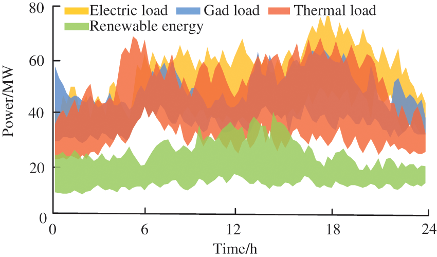
Figure 4: Historical sample data of IES

The training results of the TD3 algorithm are shown in Fig. 5. The reward value obtained by the agent at the initial stage of training is relatively low. The TD3 algorithm gets a stable optimal solution when the episodes approaching about 3000.

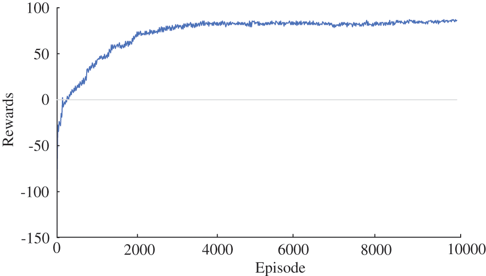
Figure 5: The cumulative reward value of agents

4.2 Scenario Analysis

To verify the effectiveness of the proposed multi-objective low-carbon scheduling method, the scheduling results of five different operating scenarios are compared.

Scenario 1: The optimization objective is the operation cost, and the economy of system operation is considered in the optimization process.

Scenario 2: CCP combined optimization model is utilized.

Scenario 3: Power supply reliability is considered based on scenario 2.

Scenario 4: IDR is considered based on scenario 2.

Scenario 5: IDR and power supply reliability are considered based on scenario 2.

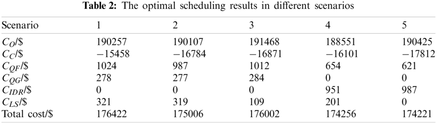
The optimal scheduling results in different scenarios are shown in Table 2. Compared with scenario 1, the system operation and total costs in scenario 2 are reduced by $150 and $1416. CCS captures CO2 emitted by CHP, and transmits it to P2G, thus saving the cost of P2G transmission and purchasing CO2. Compared with scenario 2, the total cost of the system in scenario 3 is increased by $996 to meet load requirements after considering system reliability. Compared with scenario 2, the power load demand in the peak period and the starting capacity of CHP units in scenario 4 are reduced. Compared with scenario 2, the load rejection of the system in scenario 5 is reduced to 0, and the wind curtailment cost is significantly reduced. At the same time, the PV curtailment costs are reduced to 0, and the total cost of the IES is reduced by $2201. Therefore, the method proposed can improve the reliability of the power supply and economic benefits.

CO2 emissions in different scenarios are shown in Fig. 6. In the load peak period (20:00–22:00), scenario 2 emits less CO2 than scenario 1 as the requirements of CO2 of P2G come from CCS. Scenario 4 has the lowest CO2 emissions due to the less CHP unit output during peak load periods. Scenario 3 considers the power supply reliability, improves the output of CHP units, resulting in the highest CO2 emissions. Considering power supply reliability and IDR, scenario 5 has slightly higher carbon emissions than scenario 4, but lower than scenario 2.

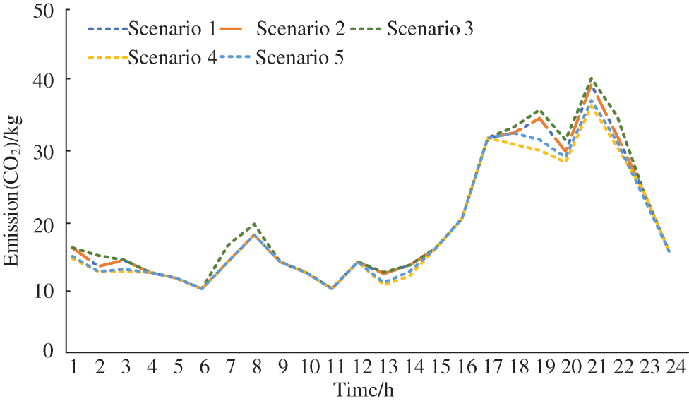
Figure 6: CO2 emissions in different scenarios

The load shedding rate in different scenarios is shown in Fig. 7. The load shedding rates in scenario 1 are the same as scenario 2, and the CCP combined optimization model does not affect power supply stability. In CCP combined optimization model, the electric power consumed by P2G and CCS is directly taken from electric power generated by CHP. The integrated energy system generates and consumes no additional power. Compared with scenario 1, the operation stability of the IES in scenario 3 is improved by considering the power supply reliability. Compared with scenario 1, the load demand in scenario 4 is less during the period (7:00–8:00, 19:00–22:00), and the power supply reliability is improved after considering the demand response.

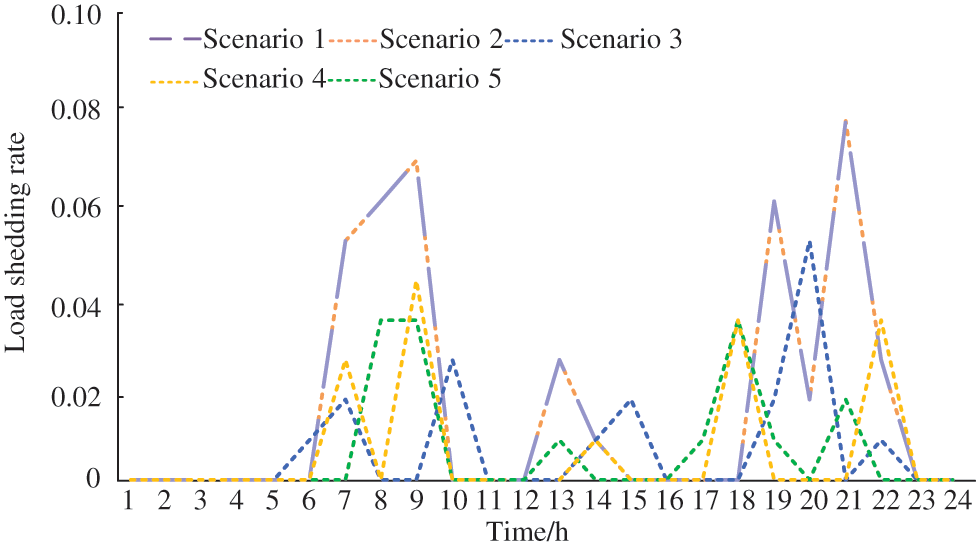
Figure 7: The load shedding rate in different scenarios

The scheduling results of the IES in different scenarios are shown in Fig. 8. In scenario 3, CHP unit output is significantly higher than other scenarios thanks to the consideration of power supply reliability. In scenario 4, the outputs of CHP units during peak load period are lower than those of other scenarios, and the outputs of renewable energy are higher than those of other scenarios during under load period due to the considerations of power supply reliability and IDR. In scenario 5, during the underestimation period (0:00–06:00) of load, the peak load demand is transferred to the underestimation period after demand response, and renewable energy outputs are significantly higher than those in other scenarios. During the peak load period (19:00–21:00), CO2 emissions are reduced while maintaining system reliability. The optimization method based on TD3 can achieve a better control effect in different scenarios.

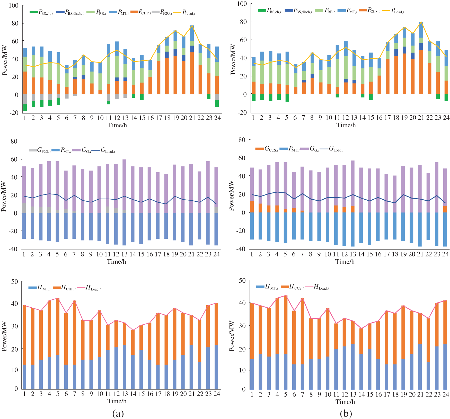
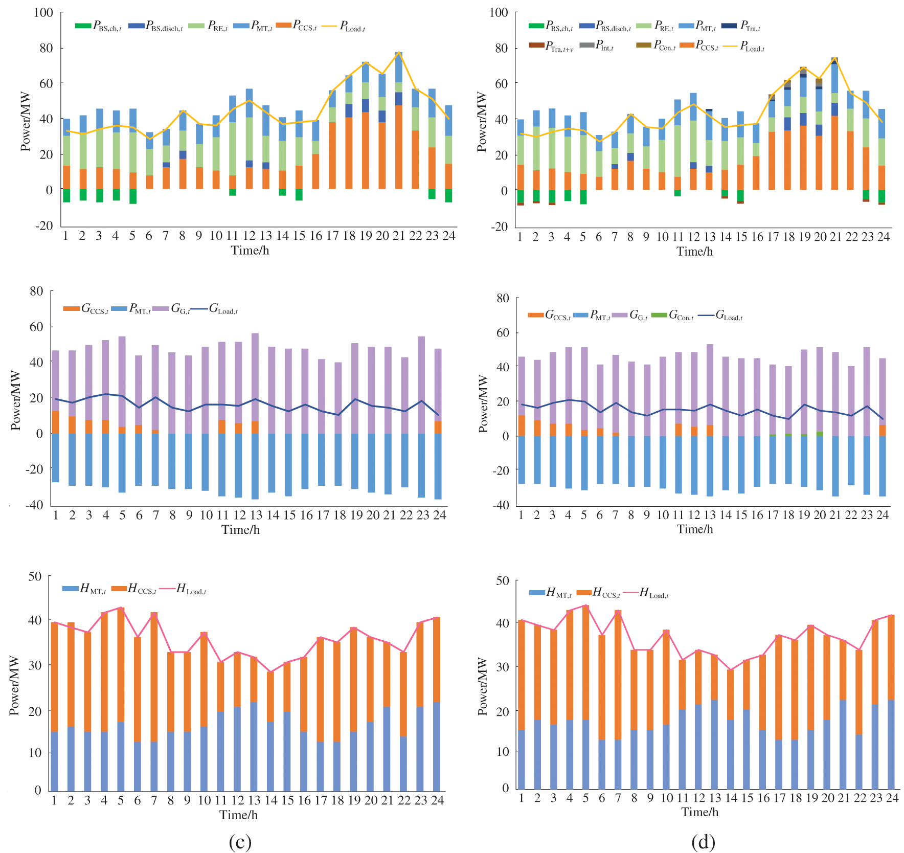
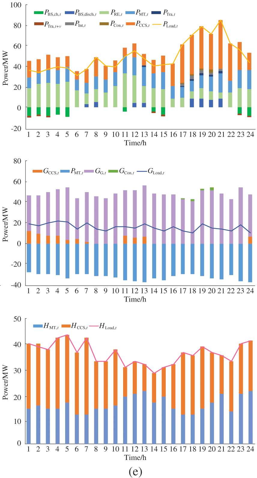
Figure 8: The power balances of the IES in different scenarios. (a) The power balances of the IES in scenario 1, (b) the power balances of the IES in scenario 2, (c) the power balances of the IES in scenario 3, (d) the power balances of the IES in scenario 4, (e) the power balances of the IES in scenario 5

4.3 Comparison Analysis

SAC, A3C, DDPG and DQN algorithms are selected to verify the effectiveness of the proposed low carbon optimization model. The parameters of SAC, A3C, DDPG and DQN are taken from the literature [29–32].

The reward curves of different comparison methods are shown in Fig. 9. The reward values obtained by DDPG and SAC algorithms are similar in convergence. The convergence speed of the A3C algorithm is higher than other methods due to the asynchronous architecture. The proposed optimization method based on TD3 has the best comprehensive performance and can obtain higher reward values.

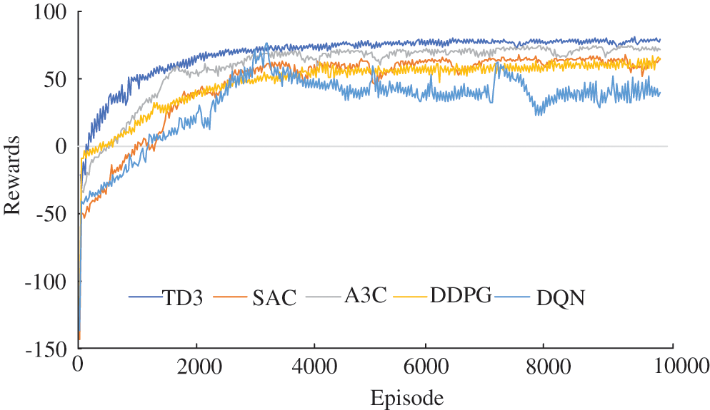
Figure 9: Reward curve in the training process of different algorithms

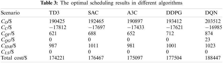
The optimal scheduling results in different algorithms are shown in Table 3. DQN algorithm has the highest operating cost due to the discretization of the agent action. The optimization results of the SAC algorithm and DDPG algorithm are similar, and the wind power curtailment cost of DDPG is higher than the SAC algorithm. A3C algorithm uses asynchronous mechanism, so the operating cost is lower than DQN, DDPG, and SAC algorithms. TD3 algorithm has the lowest cost and, obtains higher carbon emission benefits.

5  Conclusions

In this paper, a multi-objective optimization method based on TD3 is proposed for the low-carbon scheduling problem of the IES. On the power generation side, we develop the CCP combined optimization model. IDR and power supply reliability are considered on the power supply side. Moreover, we describe the multi-objective optimization problem as MDP and use the deep reinforcement learning method based on TD3 to solve it. The proposed method can achieve a better control effect in different scenarios. The results show that the proposed method saves the operation cost of the system and effectively reduces the CO2 emission of the IES. Compared with TD3, SAC, A3C, DDPG and DQN algorithms, the operating costs are reduced by 8.6%, 4.3%, 6.1% and 8.0%, respectively.

Funding Statement: This work was supported in part by the Scientific Research Fund of Liaoning Provincial Education Department under Grant LQGD2019005, in part by the Doctoral Start-up Foundation of Liaoning Province under Grant 2020-BS-141.

Conflicts of Interest: The authors declare that they have no conflicts of interest to report regarding the present study.

This work is licensed under a Creative Commons Attribution 4.0 International License, which permits unrestricted use, distribution, and reproduction in any medium, provided the original work is properly cited.