| Computer Modeling in Engineering & Sciences |
DOI: 10.32604/cmes.2022.020756
ARTICLE
RBMDO Using Gaussian Mixture Model-Based Second-Order Mean-Value Saddlepoint Approximation
1School of Mechanical and Electrical Engineering, University of Electronic Science and Technology of China, Chengdu, 611731, China
2Failure Mechanics & Engineering Disaster Prevention and Mitigation, Key Laboratory of Sichuan Province, Sichuan University, Chengdu, 610065, China
3Yangzhou Yangjie Electronic Technology Co., Ltd., Yangzhou, 225008, China
4Sichuan Special Equipment Inspection and Research Institute, Chengdu, 610100, China
5Food Safety Inspection Technology Center of Administration for Market Regulation of Sichuan Province, Chengdu, 610017, China
*Corresponding Author: Tao Lin. Email: dzkdmdb@163.com
Received: 10 December 2021; Accepted: 13 January 2022
Abstract: Actual engineering systems will be inevitably affected by uncertain factors. Thus, the Reliability-Based Multidisciplinary Design Optimization (RBMDO) has become a hotspot for recent research and application in complex engineering system design. The Second-Order/First-Order Mean-Value Saddlepoint Approximate (SOMVSA/FOMVSA) are two popular reliability analysis strategies that are widely used in RBMDO. However, the SOMVSA method can only be used efficiently when the distribution of input variables is Gaussian distribution, which significantly limits its application. In this study, the Gaussian Mixture Model-based Second-Order Mean-Value Saddlepoint Approximation (GMM-SOMVSA) is introduced to tackle above problem. It is integrated with the Collaborative Optimization (CO) method to solve RBMDO problems. Furthermore, the formula and procedure of RBMDO using GMM-SOMVSA-Based CO(GMM-SOMVSA-CO) are proposed. Finally, an engineering example is given to show the application of the GMM-SOMVSA-CO method.
Keywords: Uncertain factors; reliability-based multidisciplinary design optimization; saddlepoint approximate; gaussian mixture model; collaborative optimization
Multidisciplinary Design Optimization (MDO) is a methodology that deals with complex and coupled engineering system design problems [1,2]. MDO uses the cooperative mechanism of interaction to design complex systems and subsystems to improve product performance [3,4]. In actual engineering, the exchange of information between coupled disciplines will lead to the spread of uncertain factors [5–8]. However, in the original MDO method, the influence of uncertain factors is ignored, which may lead to product failure [9–11]. The Reliability-Based Multidisciplinary Design Optimization (RBMDO) method is proposed to deal with the influence of uncertain factors [12–23]. In RBMDO, reliability analysis methods mainly include three methods: the analytical method, the approximate analytical method, and the simulation method [24–27]. The analytical method can be used to handle simple reliability constraints. The simulation method requires lots of samples to obtain accurate analysis results [28]. The approximate analytical method is widely used because of its balance between calculation accuracy and efficiency [29,30].
Approximate analytical methods in multidisciplinary reliability analysis methods include First-Order/Second-Order Mean-Value Reliability Analysis (FOMVRA/SOMVRA) methods [31]. However, both of them require the Rosenblatt transformation, which may add to the complexity of the Limit State Function (LSF), resulting in low accuracy for uncertainty analysis [32,33]. To tackle this problem, Huang et al. [34] proposed a First-Order Mean-Value Saddlepoint Approximation (FOMVSA) method. Papadimitriou [35] proposed a Second-Order Mean-Value Saddlepoint Approximation (SOMVSA) method to increase the calculated precision of the FOMVSA method. In SOMVSA, however, only when the distribution of input random variables is Gaussian distribution can the output Moment Generating Function (MGF) be directly expressed by the input MGF.
To deal with this problem, Papadimitriou et al. [36] proposed a Gaussian Mixture Model-based Second-Order Mean-Value Saddlepoint Approximation (GMM-SOMVSA) method by using a Gaussian mixture model instead of randomly distributed random variables. Thus, in this study, the GMM-SOMVSA method is introduced and is integrated with the Collaborative Optimization (CO) method [37–39] to solve RBMDO problems. Furthermore, the formula and procedure of RBMDO using GMM-SOMVSA-Based CO (GMM-SOMVSA-CO) are proposed.
The other parts of this paper are organized as follows. In Section 2, MDO and RBMDO models are introduced. Current reliability assessment methods in RBMDO are also reviewed. In Section 3, the computational procedure of GMM-SOMVSA is introduced. In Section 4, the proposed method is explained, namely, the RBMDO method combining GMM-SOMVSA and CO (GMM-SOMVSA-CO). In Section 5, the calculated precision of the proposed method is proved using an engineering example. Finally, Section 6 concludes the paper.
2 The Emulation and Approximation Ways for the Reliability Assessment in RBMDO Issues
The RBMDO model is shown in Eq. (1).
where:
2.2 Emulation and Approximation Ways for the Reliability Assessment
The reliability
where:
Joint PDF is non-linear and random variables are multi-dimensional [40]. Therefore, under the modern scientific system, it is not easy to directly find the solution of Eq. (2). Currently, three strategies are often used to estimate
3 The Reliability Evaluation Method with GMM-SOMVSA
FOMVSA only uses the first two sample points of random variables as the research objects [47]. The Cumulative Distribution Function (CDF) and PDF of the LSF can be obtained by SA. And use of the MGF of the input random variables to compute the MGF of the LSF is allowed. These features make the computational procedure simple and clear; thus, it can roughly solve RBMDO problems. The detailed computational procedure is as follows:
Step I: Linearize the LSF. Linearized LSF using first-order Taylor expansion at the deterministic variable's value or the random variable's mean. The expansion expression is shown in Eq. (3) [34]:
where:
Step II: Calculate the Cumulative Generating Function (CGF) of the LSF. If the CGF of the random variable
where:
where:
Two important functional properties of CGF are given below to further illustrate the role of CGF in the reliability analysis method based on SA [34]:
Property 1: If the random variables in the variable space
Property 2: If
By these two properties, the CGF of
Find the solution where the first derivative of the above formula is equal to zero:
Step III: Calculate the PDF and CDF of the LSF. Through Eq. (7), the value of saddlepoint
where:
The failure probability (CDF of the LSF) can be obtained by Eqs. (9) or (10):
where:
In this method, the cost of calculating the limit state gradient is independent of the number of random variables. Only the first-order sensitivity derivative of the random variables needs to be input. Therefore, the most significant superiority of the FOMVSA method is that it reduces the computational cost [34]. Nevertheless, this method only uses Taylor first-order expansion, which leads to poor approximation of the LSF. This problem is especially notable when the variance of the random variables is large. Thus, this method is appropriate only when the standard deviation of random variables is small and the uncertainty of the model is low.
To improve the calculation accuracy of FOMVSA, SOMVSA method is proposed [35]. Compared with FOMVSA, this method has a more accurate approximate solution. And it can also solve the problem that FOMVSA cannot handle the large standard deviation of random variables [48]. The detailed computational procedure is as follows:
Step I: Linearize the LSF. Linearized LSF using second-order Taylor expansion at the deterministic variable's value or the random variable's mean. Its expression is as follows:
After simplifying the above equation, as shown in Eq. (13):
Express the above equation as a matrix polynomial form, as shown in Eq. (14):
The parameter expression is as follows:
Step II: Calculate the CGF of the LSF. Through the above derivation process, the MGF of the LSF
where:
Step III: Calculate the PDF and CDF of the LSF. Take the derivative of the CGF of the LSF
It should be noted that only when the input distribution is Gaussian input distribution can the SOMVSA method directly use the MGF of the input random variables to represent the output MGF like FOMVSA. Therefore, SOMVSA is only valid when the distribution of input variables is Gaussian distribution.
Regarding the problem that MVSOSA cannot handle non-Gaussian input variables, the GMM-SOMVSA method is proposed [36]. This method uses the Expectation Maximization (EM) algorithm to find the parameters of the Gaussian mixture model, thereby transforming the joint distribution of non-Gaussian inputs into the Gaussian mixture model. Finally, the MVSOSA method is used to solve the reliability of the system. The detailed steps are as follows:
Step I: Extract a sample of size M from the copula function
Step II: Use the inverse marginal CDFs and produce a sample
where:
Step III: Apply the EM algorithm to solve the parameters
Expected steps:
Maximization steps:
where: i represents the ith cycle;
The corresponding parameters are updated once every iteration. The iterative convergence conditions of the algorithm are as follows:
where:
Step IV: Linearize the LSF. From Eq. (14), the expanded LSF can be obtained.
Step V: Calculate the CGF of the expanded LSF.
The MGF of LSF can be expressed as follows:
where:
Take the natural logarithm of
Step VI: Calculate the PDF and CDF of the LSF. First, take the derivative of the CGF of the LSF
4 The Procedure of GMM-SOMVSA-CO
The GMM-SOMVSA is integrated with the CO method to solve the RBMDO problem, namely GMM-SOMVSA-CO method.
The solving procedure of GMM-SOMVSA-CO is as follows:
Step I: Set the initial value of the design variables
Step II: System-level optimization. The optimization model is as follows:
where:
Step III: Discipline-level optimization. The solution obtained by Eq. (24) is the design parameter of the ith discipline. The optimization model is as follows:
The reliability analysis at the discipline-level can be divided into 6 steps: (1) Extract a sample of size M from the copula function
Step IV: Determine whether the algorithm has converged. The solution
The GMM-SOMVSA-CO solution procedure is shown in Fig. 1.

Figure 1: GMM-SOMVSA-CO solution procedure
This example is the design optimization of the working device of a mining excavator. The actual picture and structure diagram of the mining excavator are shown in Figs. 2 and 3, respectively. The working device of the excavator consists of a lifting mechanism and a pushing mechanism. The mechanism composition and movement principle of the working device are shown in Fig. 4. The purpose of optimization is to maximize the lifting force

Figure 2: Actual pictures of mining excavator [49]

Figure 3: Schematic diagram of mining excavator structure

Figure 4: The mechanism composition and movement principle of the excavator working device
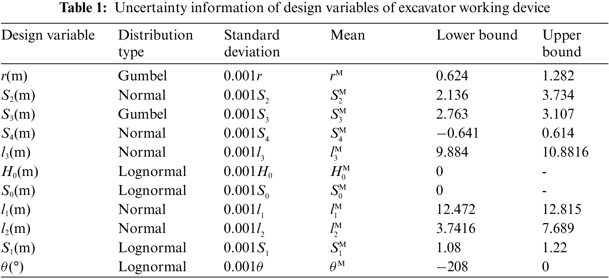
This optimization design has 11 design variables: r,
Divide this optimization problem into two disciplines, as shown in Fig. 5. Therefore, lifting discipline is discipline 1; pushing discipline is discipline 2.

Figure 5: Disciplinary division of optimization problems
The mathematical model of this optimization problem is shown as follows:
where: q is the standard excavating bucket capacity;
The system-level and discipline-level optimization mathematical model can be expressed by Eqs. (27)–(29).
The optimization model of the system layer is:
The optimization model of discipline 1 is:
The optimization model of discipline 2 is:
The target reliability is 0.98. The calculated results of GMM-SOMVSA-CO are contrasted with MCS-CO and FOMVSA-CO in Tables 2 and 3.
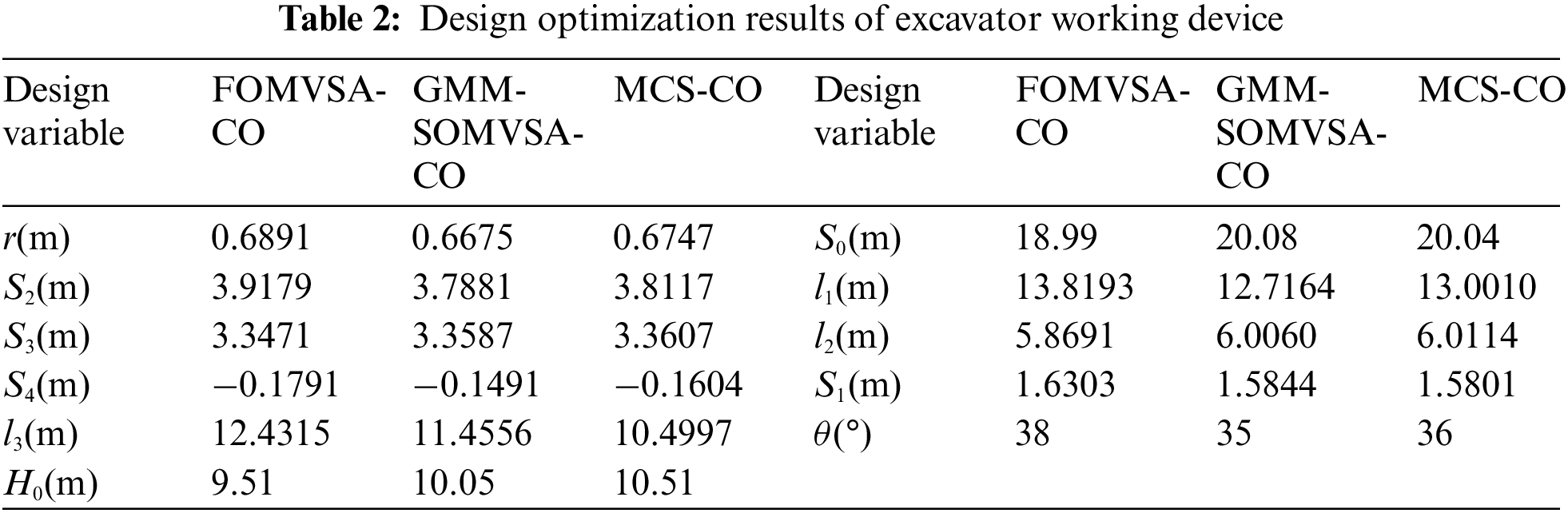
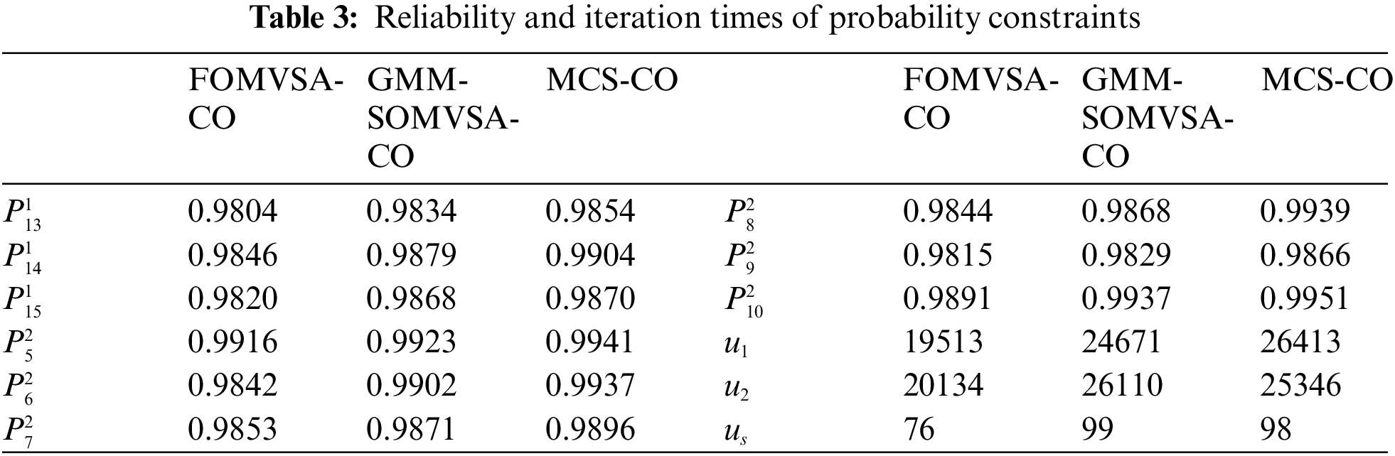
The reliability indexes of the three methods all meet the requirements of the example. However, compared with the FOMVSA-CO method, the GMM-SOMVSA-CO method and the MCS-CO method are more reliable. In addition, the solution result of the GMM-SOMVSA-CO method is closer to the solution result of the MCS-CO method, which indicates that the GMM-SOMVSA-CO method has higher accuracy.
In this paper, GMM-SOMVSA-CO is proposed to solve RBMDO issues. The proposed method introduces an EM algorithm to find the parameters of the Gaussian mixture distribution. Then the non-Gaussian input joint distribution is transformed into a Gaussian mixture distribution. Finally, the response MGF is computed to reckon the reliability of the system. This paper also gives the detailed computational procedure and mathematical model of GMM-SOMVSA-CO. An engineering example is used to show the application of the GMM-SOMVSA-CO. The GMM-SOMVSA-CO method mainly has three advantages. First, GMM-SOMVSA-CO has high solution accuracy. Second, it can solve the problem that SOMVSA cannot handle (the non-normal Gaussian distribution). Third, the optimization process of the GMM-SOMVSA-CO method is consistent with the existing engineering design division. The optimization problem of each discipline level represents a certain discipline field in the actual design problem. It is not necessary to consider the influence of other disciplines in the analysis and optimization of a single discipline.
Funding Statement: The support from the National Natural Science Foundation of China (Grant No. 52175130), the Sichuan Science and Technology Program (Grant No. 2021YFS0336), the China Postdoctoral Science Foundation (Grant No. 2021M700693), the 2021 Open Project of Failure Mechanics and Engineering Disaster Prevention, Key Lab of Sichuan Province (Grant No. FMEDP202104), the Fundamental Research Funds for the Central Universities (Grant No. ZYGX2019J035), the Sichuan Science and Technology Innovation Seedling Project Funding Project (Grant No. 2021112) and the Sichuan Special Equipment Inspection and Research Institute (YNJD-02-2020) are gratefully acknowledged.
Conflicts of Interest: The authors declare that they have no conflicts of interest to report regarding the present study.
1. Sun, X., Shi, Z., Lei, G., Guo, Y., Zhu, J. (2020). Multi-objective design optimization of an IPMSM based on multilevel strategy. IEEE Transactions on Industrial Electronics, 68(1), 139–148. DOI 10.1109/TIE.41. [Google Scholar] [CrossRef]
2. Ai, Q., Yuan, Y., Shen, S. L., Wang, H., Huang, X. (2020). Investigation on inspection scheduling for the maintenance of tunnel with different degradation modes. Tunnelling and Underground Space Technology, 106, 103589. DOI 10.1016/j.tust.2020.103589. [Google Scholar] [CrossRef]
3. Li, Y. H., Sheng, Z., Zhi, P., Li, D. (2021). Multi-objective optimization design of anti-rolling torsion bar based on modified NSGA-III algorithm. International Journal of Structural Integrity, 12(1), 17–30. DOI 10.1108/IJSI-03-2019-0018. [Google Scholar] [CrossRef]
4. Zhi, P., Li, Y., Chen, B., Li, M., Liu, G. (2019). Fuzzy optimization design-based multi-level response surface of bogie frame. International Journal of Structural Integrity, 10(2), 134–148. DOI 10.1108/IJSI-10-2018-0062. [Google Scholar] [CrossRef]
5. Teng, J., Jakeman, A. J., Vaze, J., Croke, B. F., Dutta, D. et al. (2017). Flood inundation modelling: A review of methods, recent advances and uncertainty analysis. Environmental Modelling & Software, 90, 201–216. DOI 10.1016/j.envsoft.2017.01.006. [Google Scholar] [CrossRef]
6. Liu, X., Wang, X., Xie, J., Li, B. (2020). Construction of probability box model based on maximum entropy principle and corresponding hybrid reliability analysis approach. Structural and Multidisciplinary Optimization, 61(2), 599–617. DOI 10.1007/s00158-019-02382-9. [Google Scholar] [CrossRef]
7. Xiao, F. (2019). A distance measure for intuitionistic fuzzy sets and its application to pattern classification problems. IEEE Transactions on Systems, Man, and Cybernetics: Systems, 51(6), 3980–3992. DOI 10.1109/TSMC.2019.2958635. [Google Scholar] [CrossRef]
8. Zhou, Q., Deng, Y. (2021). Higher order information volume of mass function. Information Sciences, 586, 501–513. DOI 10.1016/j.ins.2021.12.005. [Google Scholar] [CrossRef]
9. Keshtegar, B., Hao, P. (2017). A hybrid self-adjusted mean value method for reliability-based design optimization using sufficient descent condition. Applied Mathematical Modelling, 41, 257–270. DOI 10.1016/j.apm.2016.08.031. [Google Scholar] [CrossRef]
10. Meng, D., Hu, Z., Guo, J., Lv, Z., Xie, T. et al. (2021). An uncertainty-based structural design and optimization method with interval taylor expansion. Structures, 33, 4492–4500. DOI 10.1016/j.istruc.2021.07.007. [Google Scholar] [CrossRef]
11. Alirahmi, S. M., Dabbagh, S. R., Ahmadi, P., Wongwises, S. (2020). Multi-objective design optimization of a multi-generation energy system based on geothermal and solar energy. Energy Conversion and Management, 205, 112426. DOI 10.1016/j.enconman.2019.112426. [Google Scholar] [CrossRef]
12. Manouchehry Nya, R., Abdullah, S., Singh, S. K. S. (2019). Reliability-based fatigue life of vehicle spring under random loading. International Journal of Structural Integrity, 10(5), 737–748. DOI 10.1108/IJSI-03-2019-0025. [Google Scholar] [CrossRef]
13. Xiao, F. (2021). CEQD: A complex mass function to predict interference effects. IEEE Transactions on Cybernetics, 1–13. DOI 10.1109/TCYB.6221036. [Google Scholar] [CrossRef]
14. Zhu, S. P., Keshtegar, B., Trung, N. T., Yaseen, Z. M., Bui, D. T. (2021). Reliability-based structural design optimization: Hybridized conjugate mean value approach. Engineering with Computers, 37(1), 381–394. DOI 10.1007/s00366-019-00829-7. [Google Scholar] [CrossRef]
15. Xie, D., Xiao, F., Pedrycz, W. (2022). Information quality for intuitionistic fuzzy values with its application in decision making. Engineering Applications of Artificial Intelligence, 109, 104568. DOI 10.1016/j.engappai.2021.104568. [Google Scholar] [CrossRef]
16. Li, L., Wan, H., Gao, W., Tong, F., Li, H. (2019). Reliability based multidisciplinary design optimization of cooling turbine blade considering uncertainty data statistics. Structural and Multidisciplinary Optimization, 59(2), 659–673. DOI 10.1007/s00158-018-2081-5. [Google Scholar] [CrossRef]
17. Deng, J., Deng, Y., Cheong, K. H. (2021). Combining conflicting evidence based on Pearson correlation coefficient and weighted graph. International Journal of Intelligent Systems, 36(12), 7443–7460. DOI 10.1002/int.22593. [Google Scholar] [CrossRef]
18. Meng, D., Xie, T., Wu, P., He, C., Hu, Z. et al. (2021). An uncertainty-based design optimization strategy with random and interval variables for multidisciplinary engineering systems. Structures, 32, 997–1004. DOI 10.1016/j.istruc.2021.03.020. [Google Scholar] [CrossRef]
19. Hu, X., Chen, X., Parks, G. T., Yao, W. (2016). Review of improved monte carlo methods in uncertainty-based design optimization for aerospace vehicles. Progress in Aerospace Sciences, 86, 20–27. DOI 10.1016/j.paerosci.2016.07.004. [Google Scholar] [CrossRef]
20. Xiao, F. (2021). Caftr: A fuzzy complex event processing method. International Journal of Fuzzy Systems, 1–14. DOI 10.1007/s40815-021-01118-6. [Google Scholar] [CrossRef]
21. Meng, D., Lv, Z., Yang, S., Wang, H., Xie, T. et al. (2021). A time-varying mechanical structure reliability analysis method based on performance degradation. Structures, 34, 3247–3256. DOI 10.1016/j.istruc.2021.09.085. [Google Scholar] [CrossRef]
22. He, J. C., Zhu, S. P., Liao, D., Niu, X. P. (2020). Probabilistic fatigue assessment of notched components under size effect using critical distance theory. Engineering Fracture Mechanics, 235, 107150. DOI 10.1016/j.engfracmech.2020.107150. [Google Scholar] [CrossRef]
23. Meng, D., Li, Y., He, C., Guo, J., Lv, Z. et al. (2021). Multidisciplinary design for structural integrity using a collaborative optimization method based on adaptive surrogate modelling. Materials & Design, 206, 109789. DOI 10.1016/j.matdes.2021.109789. [Google Scholar] [CrossRef]
24. Pan, L., Deng, Y. (2022). A novel similarity measure in intuitionistic fuzzy sets and its applications. Engineering Applications of Artificial Intelligence, 107, 104512. DOI 10.1016/j.engappai.2021.104512. [Google Scholar] [CrossRef]
25. Su, X., Li, L., Shi, F., Qian, H. (2018). Research on the fusion of dependent evidence based on mutual information. IEEE Access, 6, 71839–71845. DOI 10.1109/Access.6287639. [Google Scholar] [CrossRef]
26. Bagheri, M., Zhu, S. P., Ben Seghier, M. E. A., Keshtegar, B., Trung, N. T. (2021). Hybrid intelligent method for fuzzy reliability analysis of corroded x100 steel pipelines. Engineering with Computers, 37(4), 2559–2573. DOI 10.1007/s00366-020-00969-1. [Google Scholar] [CrossRef]
27. Yang, Y. J., Wang, G., Zhong, Q., Zhang, H., He, J. et al. (2021). Reliability analysis of gas pipeline with corrosion defect based on finite element method. International Journal of Structural Integrity, 12(6), 854–863. DOI 10.1108/IJSI-11-2020-0112. [Google Scholar] [CrossRef]
28. Abd Rahim, A. A., Abdullah, S., Singh, S. S. K., Nuawi, M. Z. (2019). Reliability assessment on automobile suspension system using wavelet analysis. International Journal of Structural Integrity, 10(5), 602–611. DOI 10.1108/IJSI-04-2019-0035. [Google Scholar] [CrossRef]
29. Liu, X., Liu, X., Zhou, Z., Hu, L. (2021). An efficient multi-objective optimization method based on the adaptive approximation model of the radial basis function. Structural and Multidisciplinary Optimization, 63(3), 1385–1403. DOI 10.1007/s00158-020-02766-2. [Google Scholar] [CrossRef]
30. Liao, D., Zhu, S. P., Keshtegar, B., Qian, G., Wang, Q. (2020). Probabilistic framework for fatigue life assessment of notched components under size effects. International Journal of Mechanical Sciences, 181, 105685. DOI 10.1016/j.ijmecsci.2020.105685. [Google Scholar] [CrossRef]
31. Liu, X., Gong, M., Zhou, Z., Xie, J., Wu, W. (2021). An improved first order approximate reliability analysis method for uncertain structures based on evidence theory. Mechanics Based Design of Structures and Machines, 1–18. DOI 10.1080/15397734.2021.1956324. [Google Scholar] [CrossRef]
32. Yuan, R., Tang, M., Wang, H., Li, H. (2019). A reliability analysis method of accelerated performance degradation based on Bayesian strategy. IEEE Access, 7, 169047–169054. DOI 10.1109/Access.6287639. [Google Scholar] [CrossRef]
33. Cheng, C., Xiao, F. (2021). A distance for belief functions of orderable set. Pattern Recognition Letters, 145, 165–170. DOI 10.1016/j.patrec.2021.02.010. [Google Scholar] [CrossRef]
34. Huang, B., Du, X. (2008). Probabilistic uncertainty analysis by mean-value first order saddlepoint approximation. Reliability Engineering & System Safety, 93(2), 325–336. DOI 10.1016/j.ress.2006.10.021. [Google Scholar] [CrossRef]
35. Papadimitriou, D., Mourelatos, Z. (2017). Mean-value second-order saddlepoint approximation for reliability analysis. SAE International Journal of Commercial Vehicles, 10(1), 73–80. DOI 10.4271/2017-01-0207. [Google Scholar] [CrossRef]
36. Papadimitriou, D. I., Mourelatos, Z. P., Hu, Z. (2019). Reliability analysis using second-order saddlepoint approximation and mixture distributions. Journal of Mechanical Design, 141(2), 021401. DOI 10.1115/1.4041370. [Google Scholar] [CrossRef]
37. Yuan, R., Li, H., Gong, Z., Tang, M., Li, W. (2017). An enhanced monte carlo simulation–based design and optimization method and its application in the speed reducer design. Advances in Mechanical Engineering, 9(9), 1–7. DOI 10.1177/1687814017728648. [Google Scholar] [CrossRef]
38. Meng, D., Yang, S., Zhang, Y., Zhu, S. P. (2019). Structural reliability analysis and uncertainties-based collaborative design and optimization of turbine blades using surrogate model. Fatigue & Fracture of Engineering Materials & Structures, 42(6), 1219–1227. DOI 10.1111/ffe.12906. [Google Scholar] [CrossRef]
39. Xiao, F. (2019). Multi-sensor data fusion based on the belief divergence measure of evidences and the belief entropy. Information Fusion, 46, 23–32. DOI 10.1016/j.inffus.2018.04.003. [Google Scholar] [CrossRef]
40. Meng, D., Wang, H., Yang, S., Lv, Z., Hu, Z. et al. (2022). Fault analysis of wind power rolling bearing based on EMD feature extraction. Computer Modeling in Engineering & Sciences, 130(1), 543–558. DOI 10.32604/cmes.2022.018123. [Google Scholar] [CrossRef]
41. Xiang, Y., Pan, B., Luo, L. (2020). A most probable point method for probability distribution construction. Structural and Multidisciplinary Optimization, 62(5), 2537–2554. DOI 10.1007/s00158-020-02623-2. [Google Scholar] [CrossRef]
42. Liu, X., Liang, R., Hu, Y., Tang, X., Bastien, C. et al. (2021). Collaborative optimization of vehicle crashworthiness under frontal impacts based on displacement oriented structure. International Journal of Automotive Technology, 22(5), 1319–1335. DOI 10.1007/s12239-021-0115-2. [Google Scholar] [CrossRef]
43. Su, X., Li, L., Qian, H., Mahadevan, S., Deng, Y. (2019). A new rule to combine dependent bodies of evidence. Soft Computing, 23(20), 9793–9799. DOI 10.1007/s00500-019-03804-y. [Google Scholar] [CrossRef]
44. Keshtegar, B., Zhu, S. P. (2019). Three-term conjugate approach for structural reliability analysis. Applied Mathematical Modelling, 76, 428–442. DOI 10.1016/j.apm.2019.06.022. [Google Scholar] [CrossRef]
45. Li, H., Yuan, R., Fu, J. (2019). A reliability modeling for multi-component systems considering random shocks and multi-state degradation. IEEE Access, 7, 168805–168814. DOI 10.1109/Access.6287639. [Google Scholar] [CrossRef]
46. Luo, C., Keshtegar, B., Zhu, S. P., Taylan, O., Niu, X. P. (2022). Hybrid enhanced monte carlo simulation coupled with advanced machine learning approach for accurate and efficient structural reliability analysis. Computer Methods in Applied Mechanics and Engineering, 388, 114218. DOI 10.1016/j.cma.2021.114218. [Google Scholar] [CrossRef]
47. Papadimitriou, D. I., Mourelatos, Z. P. (2018). Reliability-based topology optimization using mean-value second-order saddlepoint approximation. Journal of Mechanical Design, 140(3), 031403. DOI 10.1115/1.4038645. [Google Scholar] [CrossRef]
48. Hu, Z., Du, X. (2018). Saddlepoint approximation reliability method for quadratic functions in normal variables. Structural Safety, 71, 24–32. DOI 10.1016/j.strusafe.2017.11.001. [Google Scholar] [CrossRef]
49. Taiyuan Heavy Industry Co., Ltd. (2022). http://product.tyhi.com.cn/index/kssb/kyjxzcswjj/WK_35kywjj.htm. [Google Scholar]
50. Ge, L., Dong, Z., Quan, L., Li, Y. (2019). Potential energy regeneration method and its engineering applications in large-scale excavators. Energy Conversion and Management, 195, 1309–1318. DOI 10.1016/j.enconman.2019.05.079. [Google Scholar] [CrossRef]
 | This work is licensed under a Creative Commons Attribution 4.0 International License, which permits unrestricted use, distribution, and reproduction in any medium, provided the original work is properly cited. |