| Computer Modeling in Engineering & Sciences |
DOI: 10.32604/cmes.2022.020201
ARTICLE
Isogeometric Boundary Element Method for Two-Dimensional Steady-State Non-Homogeneous Heat Conduction Problem
1School of Architectural Engineering, Huanghuai University, Zhumadian, 463000, China
2College of Intelligent Construction, Wuchang University of Technology, Wuhan, 430223, China
*Corresponding Author: Yanming Xu. Email: xuyanming@ustc.edu
Received: 10 November 2021; Accepted: 08 January 2022
Abstract: The isogeometric boundary element technique (IGABEM) is presented in this study for steady-state inhomogeneous heat conduction analysis. The physical unknowns in the boundary integral formulations of the governing equations are discretized using non-uniform rational B-spline (NURBS) basis functions, which are utilized to build the geometry of the structures. To speed up the assessment of NURBS basis functions, the Bézier extraction approach is used. To solve the extra domain integrals, we use a radial integration approach. The numerical examples show the potential of IGABEM for dimension reduction and smooth integration of CAD and numerical analysis.
Keywords: Isogeometric analysis; NURBS; boundary element method; heat conduction; non-homogeneous; radial integration method
Isogeometric analysis(IGA) has garnered considerable attention in engineering research since Hughes’ pioneering study[1]. IGA employs spline functions for geometric expressions in CAD, such as non-uniform rational B-spline(NURBS) as basis functions to approximate unknown physics fields as an alternative to the usual numerical techniques based on Lagrange polynomials. IGA offers high-order consistency and versatile refinement strategies, which are very appealing in numerical simulations. IGA has been effectively implemented in numerous sectors owing to various advantages as described next[2–6]. The Bézier[7] extraction procedure has been used to increase the simulation performance and make it easier to apply IGA. Although the notion of IGA was initially established in the context of the finite element technique, its implementation in engineering practice is limited owing to its reliance on volume parameterization, which is incompatible with the boundary representation of CAD. However, the boundary element method (BEM) requires boundary parameterization and is inherently compatible with CAD models. The isogeometric boundary element method (IGABEM) has been effectively applied to a variety of domains, including linear elasticity[8–11], potential problems[12–14], fracture mechanics[15–18], electromagnetics[19], acoustics[20–29], and structural optimization[30–35], and others.
In this study, we use the NURBS method to construct a two-dimensional isogeometric model. The Bézier curve, proposed by Pierre Bézier in 1962, paved the path for the application of spline functions for modeling curved surfaces. The application of spline functions in curved surface modeling has been initiated, and NURBS has become the most widely used modeling tool in geometric modeling in the past few decades. NURBS has outstanding advantages for curved surface modeling. It can accurately represent quadratic curved surfaces, thus providing a uniform mathematical representation of regular and free surfaces. It includes a weight factor that affects the shape of curved surfaces, making it easier to control and achieve the required shape.
In this study, we focus on the heat conduction problem. Many researchers have used traditional methods to solve heat conduction problems, such as the singular boundary method for steady-state nonlinear heat conduction problems with temperature-dependent thermal conductivity[36], the combination of the BEM and radial basis function method (RBF) for the evaluation of domain integrals with boundary-only discretization[37,38], IGABEM based on NURBS for 3D steady-state thermal conduction problems for a medium with non-homogeneous inclusions[39,40], and for solving transient heat conduction problems with heat sources[41–46]. The subtraction of singularity technique is applied to compute the singular integrals in the BEM[47]. Subsequently, we have coupled RBF and IGABEM for problems of steady heat conduction with variable coefficients. RBF is used to transform the domain integral generated by variable thermal conductivity parameters and the source term into a boundary integral. The operation enables full utilization of the advantages of IGABEM with NURBS.
The remainder of this paper is organized as follows. Section 2 describes the NURBS basis functions with B-spline functions. In Section 3, the basic theory of steady-state heat conduction is described, and in Section 4, the specific operations of the domain integration treatment and the formulation of the system equations for the iterative solution are detailed. In Section 5, several numerical examples of geometric models constructed by NURBS are discussed to verify the correctness of the algorithm. Finally, the conclusions of this study are summarized in Section 6.
The principles of NURBS are briefly discussed in this section for completeness. The basis functions of NURBS are defined over a knot vector, which is a monotonic growing real number sequence, represented by
When
In Eqs. (1) and (2), p denotes the rank of the polynomial in the B-spline basis functions.
The derivative of the basis function can be written as Eq. (3):
The linear combination of NURBS basis functions and the related control points describes the B-spline curve as Eq. (4):
where,
The weight coefficient
where we have the expression for W as shown in Eq. (6):
Similar to B-spline, the NURBS curve is expressed as Eq. (7):
The rational form of the NURBS basis function, which consists of the B-spline basis function plus the weight factor
3 Integral Equations for Steady-State Inhomogeneous Heat Conduction Problems
For most materials, the thermal conductivity varies with temperature. For example, the thermal conductivity of a certain composite material at room temperature is 10.85
The steady-state heat transfer equation for an isotropic medium containing an internal heat source with temperature-dependent thermal conductivity is expressed as Eq. (8):
In Eq. (8), the thermal conductivity
In Eq. (9),
Applying the divisional integration method and Gaussian scattering theorem to the first term, we get Eq. (13):
Considering the case where the source point p is on the boundary containing the field point q, we may write Eq. (14):
4 Analytic Expressions for the Conversion of Domain Integrals to Boundary Integrals
Two domain integrals and two boundary integrals appear in the unified equation. The boundary integrals can be calculated directly by discretizing the Gauss-Legendre quadrature. However, the latter two domain integrals are due to the nonlinear thermal conductivity and heat source terms, respectively. For the domain integrals from the nonlinear thermal conductivity, as the integrals contain
4.1 Treatment of Domain Integration Due to Thermal Conductivity Nonlinearity
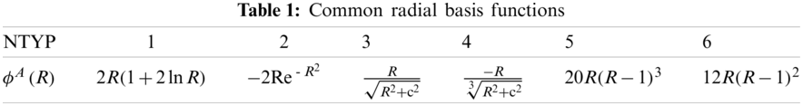
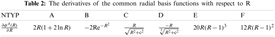
We use radial basis functions and primary polynomials to represent k, iT, which is
Here,
By applying the radial basis function in Eqs.(15) and (16) to all nodes, we obtain a set of algebraic equations written in matrix form as Eq. (17):
where
The matrix is invertible under the condition that no nodes overlap, and this is obtained by the chain rule shown in Eq. (19):
where
The temperature gradient can be expressed as Eq. (22):
in which
In Eqs.(20) and (21), the coefficients to be determined can be obtained from the collocation of the boundary and interior points, and the matrix equation can be written as Eq. (25):
In Eq. (25), the column vector of the temperature at each point can be calculated using the value of the previous iteration, and the last term of the domain integral of Eq. (14) is approximated by substitution using the radial integration method. Hence, we may write Eq. (26):
and Eq. (27):
We continue the simplification of the equation of C in Eq. (27), as shown in Eq. (28):
The original equation is thus obtained by simplifying and combining similar terms as Eq. (29):
in which, we have Eq. (30):
The Gaussian product formula is used to solve the radial integral analytically for the inverse complex quadratic radial basis function, which is usually in the form of a tight branch, as shown in Eq. (31):
It can be noted that
For Eq. (31), we use the radial integration method for the analytical solution, as shown in Eq. (32):
Fig. 1 shows the radial integration distance diagram. For a few special cases, the source point, field point, and action point are in a straight line as shown in Fig. 2. In such cases, we can solve Eq. (32) analytically. In the radial basis division method, the use of numerical integration requires considerable time, while the use of analytical solutions (as in Eq. (30)), can improve the efficiency of the calculation by several times.
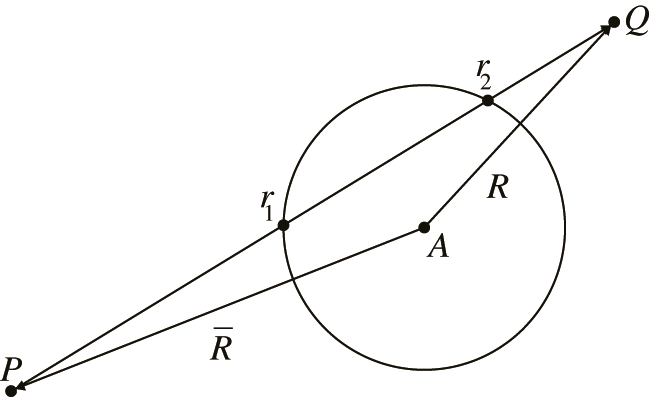
Figure 1: Schematic diagram of the starting and ending distances of radial integration
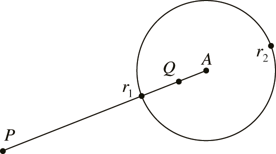
Figure 2: Special case where the tightly-supported domain intersects the radius
4.2 Processing of Domain Integrals Caused by Source Terms
We first consider the domain integral for the heat source, which is the third term on the right hand side of Eq. (14). By using the radial basis function method, the following expression can be obtained because the boundary integral can be calculated directly by Gaussian integration. We only need to consider the treatment of the domain integral. First, we consider the domain integral owing to the heat source, i.e., the second term on the right-hand side of Eq. (13) is treated using the radial basis method, and the following expression can be obtained as Eq. (33):
where
We have considered a three-dimensional problem here. Therefore, the power of r is 3-1=2. A specific derivation method can be observed in the radial basis partition. For simple heat source distribution functions, the basis function B can be derived analytically, and for complex heat source distribution functions, it can be approximated by Gaussian numerical integration.
4.3 The Set of System Equations
The unified integral boundary is discretized into Ne boundary cells, the number of boundary nodes is Nb, and the domain has Ni points. The total number of nodes is NA = Nb + Ne, NA nodes are considered as the source p in turn, and the domain integral matrix equation can be calculated, as Eq. (35):
Substituting Eq. (25) into Eq. (35), we obtain Eq. (36):
Finally, a unified system of algebraic equations is obtained, as shown in Eq. (37):
In Eq. (38), A denotes the elements in matrix
4.4 Iterative Solution of the System Equations
Solving the system of linear equations using the Newton-Raphson iteration, we assume that after the nth iteration, the residual of Eq. (38) is
For the iteration of the (n + 1)th time step and assuming the residual
We need to derive Eq. (39), and the formula can be obtained from Eq. (41):
Substituting Eq. (41) into Eq. (40), we obtain Eq. (42):
We can find the correction value of the unknown quantity
where
We consider a two-dimensional model diagram consisting of a square of 1m side length on the left and a semicircle of radius 0.5m on the right side. Additionally, there are adiabatic left and right boundaries, a constant wall temperature of 100K for the upper boundary, and three boundary conditions of 200K for the lower boundary with convective heat transfer and convective radiative heat transfer. The material density
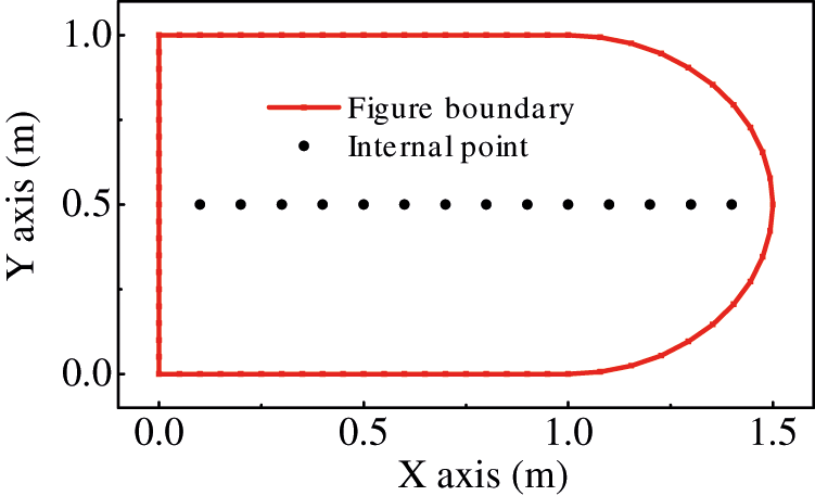
Figure 3: Two-dimensional model with interior points
The original NURBS curve and control point positions are shown in Fig. 4a. The parameter space vector of the boundary element may be produced by normalizing the knot vector, which is written as intervals of [0, 0.25), [0.25, 0.5), [0.5, 0.75), and [0.75, 1), respectively. The new control point sequence, knot vector, and weight factor vector may be produced after refinement by dividing each NURBS element evenly and inserting new knots.
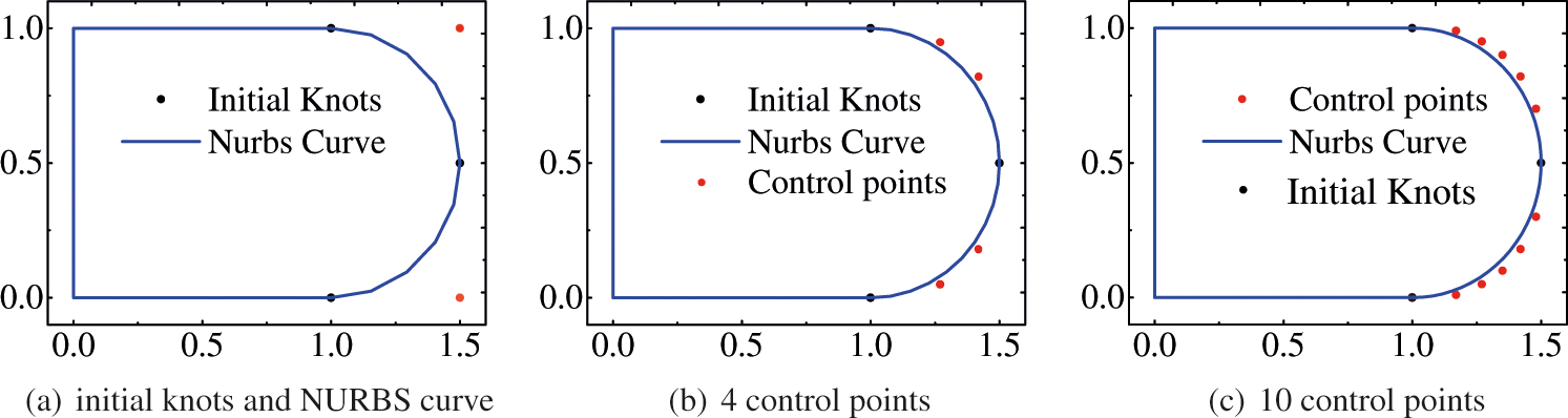
Figure 4: Plate model geometric control points with NURBS curves at various refinement levels, (a) initial knots, (b) 4 control points, (c) 10 control points
Fig. 5a shows the temperature distribution under convective boundary conditions. In the figure, near the heat source at high temperature, the temperature from the lower to upper region increases in accordance with the law of heat transfer. Fig. 5b shows the temperature distribution cloud under temperature boundary conditions. Fig. 5c shows the temperature distribution cloud under convective radiation boundary conditions and it is similar to Fig. 5a, and Fig. 6 shows the temperature of the inner point. When the boundary condition is only temperature-based, the magnitude of the temperature value is proportional to the proximity of the heat source, and when the boundary condition is based on convective or convective radiation, the temperature rises more slowly and the difference between the two is insignificant.
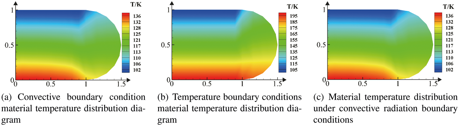
Figure 5: Distribution of homogeneous and non-homogeneous temperature under three conditions of subdivision
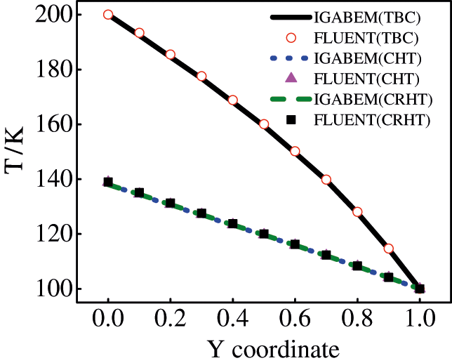
Figure 6: Temperature distribution of flat plate at x=0.5 for different lower boundary conditions
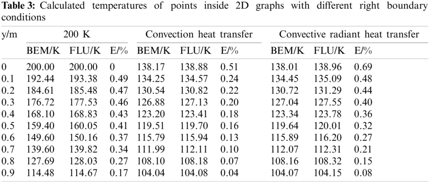
Table 3 shows the calculated temperatures of the internal points under different boundary conditions. We provide the calculated temperatures from the IGABEM and FLUENT software on the flat plate boundary. From Table3 and Fig. 6, we can observe that the IGABEM and FLUENT results have an error of less than 0.7%. Hence, the radial integration method has a high accuracy for solving two-dimensional steady-state nonlinear heat conduction problems. In Fig. 6, we refer to the temperature boundary conditions as TBC, CHT is the convective heat transfer, and CRHT is the convective radiative heat transfer.
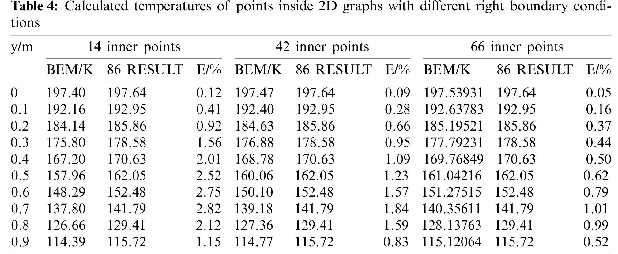
Now, we consider the temperature boundary condition as an example to study the influence of the number of internal nodes on the accuracy of the calculation results. The number of internal points is considered as 14, 42, 66, and 86 for comparison, as shown in Fig. 7, and the relative error is shown in Fig. 8 and Table 4. It is observed that compared with 86 internal points, the errors of 14 and 42 internal points are larger, with a maximum error of 2.8%, but the calculation result of 66 internal points is very close. Therefore, we can conclude that for smaller number of interior points, there is greater uncertainty in the result, and for larger number of interior points, the temperature value tends to be more stable, which verifies the correctness of the algorithm. Increasing the number of interior points can enhance computation accuracy while simultaneously increasing calculation difficulty. A topic worth investigating is how to choose the number and position of internal points. It’s tough to present the determined internal points utilizing a theoretical formulation for this problem’s examination. However, uniform distribution works effectively in most cases.
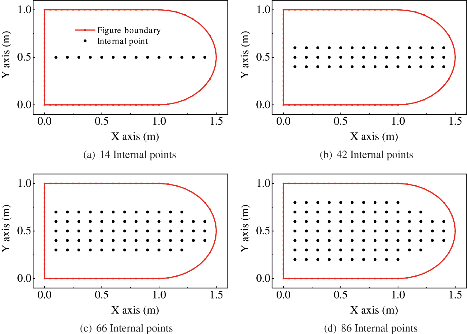
Figure 7: Mesh model with different number of interior points
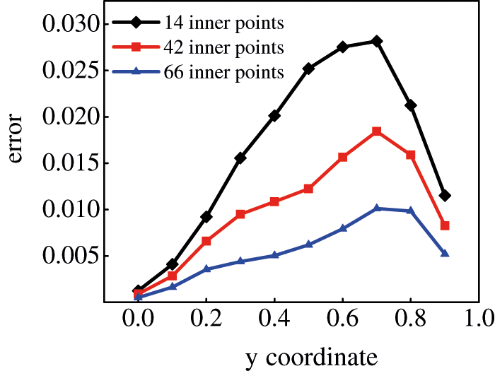
Figure 8: Relative error for models with different number of interior points
5.2 Rectangular and Semi-Elliptical Models
Let us consider a two-dimensional model diagram of rectangular and semi-elliptical models. The upper region is a rectangle of length 2m and width 1m, the lower region is a semi-ellipse and the analytical equation is
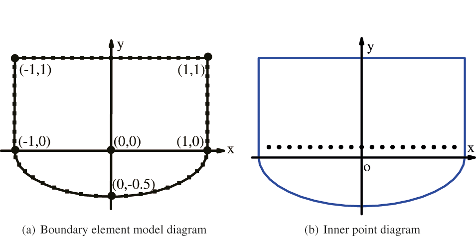
Figure 9: Boundary element model and diagram of interior points
Fig. 9a shows the model of the rectangular and semi-ellipse region. We assign the coordinates (1, 0), (1, 1), ( −1, 1), ( −1, 0), and (0, −0.5) to describe the silhouette of the plate, in order to make the calculation effective. The inner points are shown in Fig. 9b, and the coordinates of the inner points are ( −0.9, 0.1), ( −0.8, 0.1) ... (0.9, 0.1). There are a total of 19 inner points.
Fig. 10a indicates that the thermal conductivity is a constant value
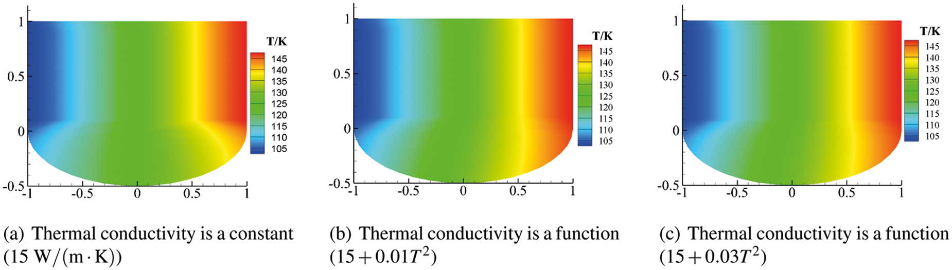
Figure 10: Cloud diagram of the effect of variable thermal conductivity on temperature
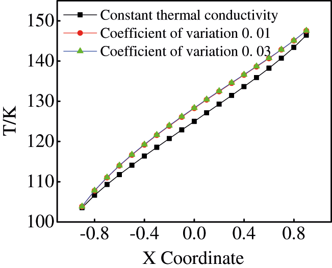
Figure 11: Effect of different coefficients on temperature values
In this study, the isogeometric boundary element technique (IGABEM) is applied to solve the two-dimensional non-homogeneous steady state heat conduction problem, and NURBS is used to construct a smooth geometric model. The radial integration method is used to transform the domain integral caused by the variable coefficient into the boundary integral. The numerical results show that the developed algorithm can effectively solve non-homogeneous steady-state heat conduction problems with variable coefficients. In the future, we will extend the algorithm to transient analysis.
Acknowledgement: The authors wish to express their appreciation to the reviewers for their helpful suggestions which greatly improved the presentation of this paper.
Funding Statement: This work is supported by Key Scientific Research Projects of Universities and Key Scientific and Technological Projects in Henan Province, which numbers are 21A440015, 22A570007 and 212102310601, respectively.
Conflicts of Interest: The authors declare that they have no conflicts of interest to report regarding the present study.
1. Hughes, T., Cottrell, J., Bazilevs, Y. (2005). Isogeometric analysis: Cad, finite elements, nurbs, exact geometry and mesh refinement. Computer Methods in Applied Mechanics and Engineering, 194(39–41), 4135–4195. DOI 10.1016/j.cma.2004.10.008. [Google Scholar] [CrossRef]
2. Cottrell, J., Hughes, T., Reali, A. (2007). Studies of refinement and continuity in isogeometric structural analysis. Computer Methods in Applied Mechanics and Engineering, 196(41–44), 4160–4183. DOI 10.1016/j.cma.2007.04.007. [Google Scholar] [CrossRef]
3. Bazilevs, Y., Calo, V., Zhang, Y., Hughes, T. (2006). Isogeometric fluid-structure interaction analysis with applications to arterial blood flow. Computational Mechanics, 38(4–5), 310–322. DOI 10.1007/s00466-006-0084-3. [Google Scholar] [CrossRef]
4. Nagy, A., Abdalla, M., Gürdal, Z. (2010). Isogeometric sizing and shape optimisation of beam structures. Computer Methods in Applied Mechanics and Engineering, 199(17–20), 1216–1230. DOI 10.1016/j.cma.2009.12.010. [Google Scholar] [CrossRef]
5. Benson, D., Bazilevs, Y., Hsu, M., Hughes, T. (2010). Isogeometric shell analysis: The reissner-mindlin shell. Computer Methods in Applied Mechanics and Engineering, 199(5–8), 276–289. DOI 10.1016/j.cma.2009.05.011. [Google Scholar] [CrossRef]
6. de Lorenzis, L., Temizer, Wriggers, P., Zavarise, G. (2011). A large deformation frictional contact formulation using nurbs-based isogeometric analysis. International Journal for Numerical Methods in Engineering, 87(13), 1278–1300. DOI 10.1002/nme.3159. [Google Scholar] [CrossRef]
7. Borden, M., Scott, M., Evans, J., Hughes, T. (2010). Isogeometric finite element data structures based on bézier extraction of nurbs. International Journal for Numerical Methods in Engineering, 87(1–5), 15–47. DOI 10.1002/nme.2968. [Google Scholar] [CrossRef]
8. Simpson, R., Bordas, S., Trevelyan, J., Rabczuk, T. (2012). A two-dimensional isogeometric boundary element method for elastostatic analysis. Computer Methods in Applied Mechanics and Engineering, 209–212, 87–100. DOI 10.1016/j.cma.2011.08.008. [Google Scholar] [CrossRef]
9. Simpson, R., Bordas, S., Lian, H., Trevelyan, J. (2013). An isogeometric boundary element method for elastostatic analysis: 2D implementation aspects. Computers & Structures, 118, 2–12. DOI 10.1016/j.compstruc.2012.12.021. [Google Scholar] [CrossRef]
10. Scott, M., Simpson, R., Evans, J., Lipton, S., Bordas, S. et al. (2013). Isogeometric boundary element analysis using unstructured t-splines. Computer Methods in Applied Mechanics and Engineering, 254, 197–221. DOI 10.1016/j.cma.2012.11.001. [Google Scholar] [CrossRef]
11. Li, S., Trevelyan, J., Zhang, W., Wang, D. (2018). Accelerating isogeometric boundary element analysis for 3-dimensional elastostatics problems through black-box fast multipole method with proper generalized decomposition. International Journal for Numerical Methods in Engineering, 114(9), 975–998. DOI 10.1002/nme.5773. [Google Scholar] [CrossRef]
12. Banerjee, P., Cathie, D. (1980). A direct formulation and numerical implementation of the boundary element method for two-dimensional problems of elasto-plasticity. International Journal of Mechanical Sciences, 22(4), 233–245. DOI 10.1016/0020-7403(80)90038-7. [Google Scholar] [CrossRef]
13. Cruse, T. (1996). Bie fracture mechanics analysis: 25 years of developments. Computational Mechanics, 18(1), 1–11. DOI 10.1007/BF00384172. [Google Scholar] [CrossRef]
14. Seybert, A., Soenarko, B., Rizzo, F., Shippy, D. (1985). An advanced computational method for radiation and scattering of acoustic waves in three dimensions. The Journal of the Acoustical Society of America, 77(2), 362–368. DOI 10.1121/1.391908. [Google Scholar] [CrossRef]
15. Nguyen, B., Tran, H., Anitescu, C., Zhuang, X., Rabczuk, T. (2016). An isogeometric symmetric galerkin boundary element method for two-dimensional crack problems. Computer Methods in Applied Mechanics and Engineering, 306, 252–275. DOI 10.1016/j.cma.2016.04.002. [Google Scholar] [CrossRef]
16. Peng, X., Atroshchenko, E., Kerfriden, P., Bordas, S. P. A. (2017). Linear elastic fracture simulation directly from CAD: 2D nurbs-based implementation and role of tip enrichment. International Journal of Fracture, 204(1), 55–78. DOI 10.1007/s10704-016-0153-3. [Google Scholar] [CrossRef]
17. Peng, X., Atroshchenko, E., Kerfriden, P., Bordas, S. P. A., Peng, X. et al. (2017). Isogeometric boundary element methods for three dimensional static fracture and fatigue crack growth. Computer Methods in Applied Mechanics and Engineering, 316, 151–185. DOI 10.1016/j.cma.2016.05.038. [Google Scholar] [CrossRef]
18. Chen, L., Wang, Z., Peng, X., Yang, J., Wu, P. et al. (2021). Modeling pressurized fracture propagation with the isogeometric bem. Geomechanics and Geophysics for Geo-Energy and Geo-Resources, 7(3), 51. DOI 10.1007/s40948-021-00248-3. [Google Scholar] [CrossRef]
19. Simpson, R., Liu, Z., Vázquez, R., Evans, J. (2018). An isogeometric boundary element method for electromagnetic scattering with compatible B-spline discretizations. Journal of Computational Physics, 362, 264–289. DOI 10.1016/j.jcp.2018.01.025. [Google Scholar] [CrossRef]
20. Simpson, R., Scott, M., Taus, M., Thomas, D., Lian, H. (2014). Acoustic isogeometric boundary element analysis. Computer Methods in Applied Mechanics and Engineering, 269, 265–290. DOI 10.1016/j.cma.2013.10.026. [Google Scholar] [CrossRef]
21. Peake, M., Trevelyan, J., Coates, G. (2015). Extended isogeometric boundary element method (xibem) for three-dimensional medium-wave acoustic scattering problems. Computer Methods in Applied Mechanics and Engineering, 284, 762–780. DOI 10.1016/j.cma.2014.10.039. [Google Scholar] [CrossRef]
22. Keuchel, S., Hagelstein, N., Zaleski, O., Von estorff, O. (2017). Evaluation of hypersingular and nearly singular integrals in the isogeometric boundary element method for acoustics. Computer Methods in Applied Mechanics and Engineering, 325, 488–504. DOI 10.1016/j.cma.2017.07.025. [Google Scholar] [CrossRef]
23. Chen, L., Marburg, S., Zhao, W., Liu, C., Chen, H. (2019). Implementation of isogeometric fast multipole boundary element methods for 2D half-space acoustic scattering problems with absorbing boundary condition. Journal of Theoretical and Computational Acoustics, 27(2), 1850024. DOI 10.1142/S259172851850024X. [Google Scholar] [CrossRef]
24. Chen, L., Lian, H., Liu, Z., Chen, H., Atroshchenko, E. et al. (2019). Structural shape optimization of three dimensional acoustic problems with isogeometric boundary element methods. Computer Methods in Applied Mechanics and Engineering, 355, 926–951. DOI 10.1016/j.cma.2019.06.012. [Google Scholar] [CrossRef]
25. Chen, L., Liu, C., Zhao, W., Liu, L. (2018). An isogeometric approach of two dimensional acoustic design sensitivity analysis and topology optimization analysis for absorbing material distribution. Computer Methods in Applied Mechanics and Engineering, 336, 507–532. DOI 10.1016/j.cma.2018.03.025. [Google Scholar] [CrossRef]
26. Jiang, F., Zhao, W., Chen, L., Zheng, C., Chen, H. (2021). Combined shape and topology optimization for sound barrier by using the isogeometric boundary element method. Engineering Analysis with Boundary Elements, 124, 124–136. DOI 10.1016/j.enganabound.2020.12.009. [Google Scholar] [CrossRef]
27. Chen, L., Lu, C., Zhao, W., Chen, H., Zheng, C. (2020). Subdivision surfaces-boundary element accelerated by fast multipole for the structural acoustic problem. Journal of Theoretical and Computational Acoustics, 28(2), 2050011. DOI 10.1142/S2591728520500115. [Google Scholar] [CrossRef]
28. Zhao, W., Chen, L., Chen, H., Marburg, S. (2020). An effective approach for topological design to the acoustic-structure interaction systems with infinite acoustic domain. Structural and Multidisciplinary Optimization, 62, 1253–1273. DOI 10.1007/s00158-020-02550-2. [Google Scholar] [CrossRef]
29. Chen, L., Zhang, Y., Lian, H., Atroshchenko, E., Ding, C. et al. (2020). Seamless integration of computer-aided geometric modeling and acoustic simulation: Isogeometric boundary element methods based on catmull-clark subdivision surfaces. Advances in Engineering Software, 149, 102879. DOI 10.1016/j.advengsoft.2020.102879. [Google Scholar] [CrossRef]
30. Li, K., Qian, X. (2011). Isogeometric analysis and shape optimization via boundary integral. Computer-Aided Design, 43(11), 1427–1437. DOI 10.1016/j.cad.2011.08.031. [Google Scholar] [CrossRef]
31. Lian, H., Kerfriden, P., Bordas, S. (2016). Implementation of regularized isogeometric boundary element methods for gradient-based shape optimization in two-dimensional linear elasticity. International Journal for Numerical Methods in Engineering, 106(12), 972–1017. DOI 10.1002/nme.5149. [Google Scholar] [CrossRef]
32. Lian, H., Kerfriden, P., Bordas, S. (2017). Shape optimization directly from cad: An isogeometric boundary element approach using T-splines. Computer Methods in Applied Mechanics and Engineering, 317, 1–41. DOI 10.1016/j.cma.2016.11.012. [Google Scholar] [CrossRef]
33. Liu, C., Chen, L., Zhao, W., Chen, H. (2017). Shape optimization of sound barrier using an isogeometric fast multipole boundary element method in two dimensions. Engineering Analysis with Boundary Elements, 85, 142–157. DOI 10.1016/j.enganabound.2017.09.009. [Google Scholar] [CrossRef]
34. Chen, L., Lu, C., Lian, H., Liu, Z., Zhao, W. et al. (2020). Acoustic topology optimization of sound absorbing materials directly from subdivision surfaces with isogeometric boundary element methods. Computer Methods in Applied Mechanics and Engineering, 362, 112806. DOI 10.1016/j.cma.2019.112806. [Google Scholar] [CrossRef]
35. Chen, L., Lian, H., Liu, Z., Gong, Y., Zheng, C. et al. (2022). Bi-material topology optimization for fully coupled structural-acoustic systems with isogeometric fem-bem. Engineering Analysis with Boundary Elements, 135, 182–195. DOI 10.1016/j.enganabound.2021.11.005. [Google Scholar] [CrossRef]
36. Mierzwiczak, M., Chen, W., Fu, Z. J. (2015). The singular boundary method for steady-state nonlinear heat conduction problem with temperature-dependent thermal conductivity. International Journal of Heat and Mass Transfer, 91, 205–217. DOI 10.1016/j.ijheatmasstransfer.2015.07.051. [Google Scholar] [CrossRef]
37. Gao, X., Wang, J. (2009). Interface integral bem for solving multi-medium heat conduction problems. Engineering Analysis with Boundary Elements, 33(4), 539–546. DOI 10.1016/j.enganabound.2008.08.009. [Google Scholar] [CrossRef]
38. Gao, X. (2006). A meshless bem for isotropic heat conduction problems with heat generation and spatially varying conductivity. International Journal for Numerical Methods in Engineering, 66(9), 1411–1431. DOI 10.1002/nme.1602. [Google Scholar] [CrossRef]
39. Gong, Y., Trevelyan, J., Hattori, G., Dong, C. (2019). Hybrid nearly singular integration for isogeometric boundary element analysis of coatings and other thin 2D structures. Computer Methods in Applied Mechanics and Engineering, 346, 642–673. DOI 10.1016/j.cma.2018.12.019. [Google Scholar] [CrossRef]
40. Gong, Y., Yang, H., Dong, C. (2018). A novel interface integral formulation for 3D steady state thermal conduction problem for a medium with non-homogenous inclusions. Computational Mechanics, 63(2), 181–199. DOI 10.1007/s00466-018-1590-9. [Google Scholar] [CrossRef]
41. An, Z., Yu, T., Bui, T., Wang, C., Trinh, N. (2018). Implementation of isogeometric boundary element method for 2-D steady heat transfer analysis. Advances in Engineering Software, 116, 36–49. DOI 10.1016/j.advengsoft.2017.11.008. [Google Scholar] [CrossRef]
42. Yu, B., Zhou, H. L., Chen, H. L., Tong, Y. (2015). Precise time-domain expanding dual reciprocity boundary element method for solving transient heat conduction problems. International Journal of Heat and Mass Transfer, 91, 110–118. DOI 10.1016/j.ijheatmasstransfer.2015.07.109. [Google Scholar] [CrossRef]
43. Cui, M., Peng, H. F., Xu, B. B., Gao, X. W., Zhang, Y. (2018). A new radial integration polygonal boundary element method for solving heat conduction problems. International Journal of Heat and Mass Transfer, 123, 251–260. DOI 10.1016/j.ijheatmasstransfer.2018.02.111. [Google Scholar] [CrossRef]
44. Yu, B., Yao, W. A., Gao, X. W., Zhang, S. (2014). Radial integration bem for one-phase solidification problems. Engineering Analysis with Boundary Elements, 39, 36–43. DOI 10.1016/j.enganabound.2013.10.018. [Google Scholar] [CrossRef]
45. Yu, B., Cao, G., Huo, W., Zhou, H., Atroshchenko, E. (2021). Isogeometric dual reciprocity boundary element method for solving transient heat conduction problems with heat sources. Journal of Computational and Applied Mathematics, 385, 113197. DOI 10.1016/j.cam.2020.113197. [Google Scholar] [CrossRef]
46. Mostafa Shaaban, A., Anitescu, C., Atroshchenko, E., Rabczuk, T. (2020). Shape optimization by conventional and extended isogeometric boundary element method with pso for two-dimensional helmholtz acoustic problems. Engineering Analysis with Boundary Elements, 113, 156–169. DOI 10.1016/j.enganabound.2019.12.012. [Google Scholar] [CrossRef]
47. Zhao, W., Chen, L., Chen, H., Marburg, S. (2019). Topology optimization of exterior acoustic-structure interaction systems using the coupled FEM-BEM method. International Journal for Numerical Methods in Engineering, 119(5), 404–431. DOI 10.1002/nme.6055. [Google Scholar] [CrossRef]
 | This work is licensed under a Creative Commons Attribution 4.0 International License, which permits unrestricted use, distribution, and reproduction in any medium, provided the original work is properly cited. |